Diphoton signals for Low Scale Gravity in Extra Dimensions

Abstract

Gravity can become strong at the TeV scale in the theory of extra dimensions. An effective Lagrangian can be used to describe the gravitational interactions below a cut-off scale. In this work, we study the diphoton production in $\gamma\gamma$, $p\bar{p}$, and $e^{+}e^{-}$ collisions in the model of low scale gravity. Since in the standard model photon-photon scattering only occurs via box diagrams, the cross section is highly suppressed. Thus, photon-photon scattering opens an interesting opportunity for studying the new gravity interaction, which allows tree-level photon couplings. In addition, we also examine the diphoton production at hadronic and $e^{+}e^{-}$ colliders. We derive the limits on the cut-off scale from the available diphoton data and also estimate the sensitivity reach in Run II at the Tevaton and at the future linear $e^{+}e^{-}$ colliders.

I Introduction

Recent advances in string theories suggest that a special 11-dimension theory (dubbed as M theory) [1] may be the theory of everything. Impacts of M theory on our present world can be studied with compactification of the 11 dimensions down to our $3+1$ dimensions. The path of compactification is, however, not unique. In this multi-dimensional world, the standard model particles live on a brane ($3+1$ dim) while there are other fields, like gravity and super Yang-Mill fields, live in the bulk. The scale at which the extra dimensions are felt is unknown, anywhere from TeV to Planck scale. Recent studies [2] show that if this scale is of order TeV and there are gauge and fermion fields living in the bulk that correspond to the Kaluza-Klein excitations of the gauge and fermion fields of the SM, early unification of gauge couplings can be realized below or even much below the original GUT scale. This is possible because the extra matters in the bulk accelerate the RGE running of the gauge couplings, which then change from logarithmic evolution to power evolution. Supersymmetry model building is also an active area in the framework of extra dimensions [3]. Apart from the above, radical ideas like TeV scale string theories were also proposed [4].

Inspired by string theories a simple but probably workable solution to the gauge hierarchy was recently proposed by Arkani-Hamed, Dimopoulos and Dvali (ADD) [5]. They assumed the space is $4+n$ dimensional, with the SM particles living on a brane. While the electromagnetic, strong, and weak forces are confined to this brane, gravity can propagate in the extra dimensions. To solve the gauge hierarchy problem they proposed the “new” Planck scale $M_{S}$ is of the order of TeV in this picture with the extra dimensions of a very large size $R$. The usual Planck scale $M_{G}=1/\sqrt{G_{N}}\sim 1.22\times 10^{19}$ GeV is related to this effective Planck scale $M_{S}$ using the Gauss’s law:

$$R^{n}\,M_{S}^{n+2}\sim M_{G}^{2}\;.$$ (1)

For $n=1$ it gives a large value for $R$, which is already ruled out by gravitational experiments. On the other hand, $n=2$ gives $R\lesssim 1$ mm, which is in the margin beyond the reach of present gravitational experiments.

The graviton including its excitations in the extra dimensions can couple to the SM particles on the brane with an effective strength of $1/M_{S}$ (instead of $1/M_{G}$) after summing the effect of all excitations collectively, and thus the gravitation interaction becomes comparable in strength to weak interaction at TeV scale. Hence, it can give rise to a number of phenomenological activities testable at existing and future colliders [6, 7, 8, 9, 10, 11, 12, 13, 14, 15, 16, 17, 18, 19, 20, 21, 22, 23]. So far, studies show that there are two categories of signals: direct and indirect. The indirect signal refers to exchanges of gravitons in the intermediate states, while direct refers to production or associated production of gravitons in the final state [6, 8, 9, 18, 20, 21]. Indirect signals include fermion pair, gauge boson pair production, correction to precision variables, etc. [6, 7, 9, 10, 11, 12, 13, 14, 15, 16, 17, 19, 22, 23]. There are also other astrophysical and cosmological signatures and constraints [24].

Processes that only occur via loop diagrams in the SM are especially interesting if the low scale gravity allows tree-level interactions. In the SM, the lowest order photon-photon scattering can only take place via box diagrams of order $\alpha^{2}$ (on amplitude level) [25] and, therefore, is highly suppressed. Thus, photon-photon scattering opens an interesting door for any tree-level photon interactions. Even if such new interactions are much weaker than the electroweak strength, these tree-level diagrams are only of order $\alpha_{\rm new}$. It stands a good chance that these new interactions can beat the standard model. In the framework of ADD, photons can scatter via exchanges of spin-2 gravitons in $s$-, $t$-, and $u$-channels and the most important is that the coupling strength can be as large as the electroweak strength. In this work, we shall study the photon-photon scattering $\gamma\gamma\to\gamma\gamma$ and demonstrate that it provides a unique channel to identify the low scale gravity interactions. Other interesting processes of the same category is $\gamma\gamma\to\nu\bar{\nu}$ and the cross-channel, $\gamma\nu\to\gamma\nu$, both of which do not have any tree-level contributions in the SM [26]. We shall not pursue these two further in this paper.

Similarly, a pair of gluons can scatter into gluons or photons via exchanges of gravitons, the latter of which is our attention at hadron colliders. The lowest order $gg\to\gamma\gamma$ scattering occurs via a $s$-channel exchange of graviton in the low scale gravity model whereas it has to be via box diagrams in the SM. Thus, the new gluon scattering will give rise to anomalous diphoton production, in addition to the $q\bar{q}\to G\to\gamma\gamma$ channel, at hadron colliders. However, the tree-level SM $q\bar{q}\to\gamma\gamma$ presents a large irreducible background, not to mention the jet-fake background. This makes the diphoton production at hadron colliders not as attractive as in $\gamma\gamma$ and $e^{+}e^{-}$ colliders as a probe to the low scale gravity model. For completeness we also study the diphoton production at $e^{+}e^{-}$ colliders.

The organization of the paper is as follows. In the next section, we compare the photon-photon scattering cross section between the SM and the low scale gravity. In Sec. III, we calculate diphoton production at the Tevatron and obtain the present limit on the cut-off scale $M_{S}$ using the diphoton data, and then estimate the sensitivity reach at the Run II. In Sec. IV, we repeat the same exercise at $e^{+}e^{-}$ colliders and obtain the limits using the diphoton data from LEPII, and estimate the sensitivity reach at the future linear $e^{+}e^{-}$ colliders. We shall then conclude in Sec. V.

II Photon-photon Scattering

We concentrate on the spin-2 component of the Kaluza-Klein (KK) states, which are the excited modes of graviton in the extra dimensions. The spin-0 component has a coupling to the gauge boson proportional to the mass of the gauge boson in the unitary gauge, which means it has a zero coupling to photons. We follow the convention in Ref.[9]. There are three contributing Feynman diagrams for the process $\gamma\gamma\to\gamma\gamma$ in the $s$-, $t$-, and $u$-channels. The amplitudes for $\gamma(p_{1})\gamma(p_{2})\to\gamma(k_{1})\gamma(k_{2})$ are given by:

$$i{\cal M}_{1} = -\frac{\kappa^{2}}{8}D(t)\,B^{\mu\nu,\mu^{\prime}\nu^{\prime}}(p_{1}-k_{1})\,\epsilon^{\rho}(p_{1})\,\epsilon^{\sigma}(p_{2})\,\epsilon^{\alpha}(k_{1})\,\epsilon^{\beta}(k_{2})\,$$ (3)

$$\times[-p_{1}\cdot k_{1}\,C_{\mu\nu,\rho\alpha}+D_{\mu\nu,\rho\alpha}(p_{1},-k_{1})]\;[-p_{2}\cdot k_{2}\,C_{\mu^{\prime}\nu^{\prime},\sigma\beta}+D_{\mu^{\prime}\nu^{\prime},\sigma\beta}(p_{2},-k_{2})]\;,$$

$$i{\cal M}_{2} = i{\cal M}_{1}(k_{1}\leftrightarrow k_{2})\;,$$ (4)

$$i{\cal M}_{3} = -\frac{\kappa^{2}}{8}D(s)\,B^{\mu\nu,\mu^{\prime}\nu^{\prime}}(p_{1}+p_{2})\,\epsilon^{\rho}(p_{1})\,\epsilon^{\sigma}(p_{2})\,\epsilon^{\alpha}(k_{1})\,\epsilon^{\beta}(k_{2})\,$$ (6)

$$\times[p_{1}\cdot p_{2}\,C_{\mu\nu,\rho\sigma}+D_{\mu\nu,\rho\sigma}(p_{1},p_{2})]\;[k_{1}\cdot k_{2}\,C_{\mu^{\prime}\nu^{\prime},\alpha\beta}+D_{\mu^{\prime}\nu^{\prime},\alpha\beta}(-k_{1},-k_{2})]\;,$$

where $\kappa=\sqrt{16\pi G_{N}}$ and $B_{\mu\nu,\rho\sigma}(k)$, $C_{\mu\nu,\rho\sigma}$ and $D_{\mu\nu,\rho\sigma}(p_{1},p_{2})$ can be found in Ref. [9]. The propagator factor $D(s)=\sum_{k}i/(s-m_{k}^{2}+i\epsilon)$, where $k$ sums over all KK levels. After some tedious algebra the square of the amplitude, summed over final and averaged over the initial helicities, is surprisingly simple:

$$\overline{\sum}|{\cal M}|^{2}=\frac{\kappa^{4}}{8}\;|D(s)|^{2}\;(s^{4}+t^{4}+u^{4})\;,$$ (7)

where we have taken $M_{S}^{2}\gg s,|t|,|u|$ and in this case the propagator factor $D(s)=D(|t|)=D(|u|)$ [9], which is given by

$$\kappa^{2}|D(s)|=\frac{16\pi}{M_{S}^{4}}\;\times{\cal F}\;,$$ (8)

where the factor ${\cal F}$ is given by

$${\cal F}=\Biggr{\{}\begin{array}[]{l}\log\left(\frac{M_{S}^{2}}{s}\right)\;\;{\rm for}\;\;n=2\;,\\ \frac{2}{n-2}\;\;\;\;\;\;\;\;\;\;\;{\rm for}\;\;n>2\;.\end{array}$$ (9)

The angular distribution is

$$\frac{d\sigma(\gamma\gamma\to\gamma\gamma)}{d|\cos\theta|}=\frac{\pi s^{3}}{M_{S}^{8}}\,{\cal F}^{2}\,\biggr{[}1+\frac{1}{8}\,(1+6\cos^{2}\theta+\cos^{4}\theta)\biggr{]}\;,$$ (10)

where $|\cos\theta|$ is from $0$ to 1. Since the cross section scales as $s^{3}/M_{S}^{8}$, which implies larger cross sections at higher $\sqrt{s}$.

The SM background calculation is well known and we do not repeat the expressions here. We used the results in Ref. [25] with the form factors from Ref. [27]. The process is via box diagrams with all charged fermions and the $W$ boson in the loop. At the low energy, the fermion contribution dominates, but once $\sqrt{s}$ gets above a hundred GeV the $W$ contribution becomes more important and completely dominates at higher $\sqrt{s}$. We show the cross sections in Fig. 1(a). This SM cross section decreases gradually when $\sqrt{s}$ is above 500 GeV. In contrast, the low scale gravity interactions give a monotonically increasing cross section. For $n=2$ and $M_{S}=4$ TeV the cross-over is at about $\sqrt{s}=600$ GeV. We notice that the signal cross section does not decrease very rapidly with $n$, unlike the production of real gravitons [8, 18].

In Fig. 1(b), we show the angular distribution for the low scale gravity and for the SM. The signal has a relatively flat distribution, as can be easily deduced from Eq. (10). The ratio of the cross section at $|\cos\theta|=0$ to that at $|\cos\theta|=1$ is only $9/16$. On the other hand, the SM background is very steep around $|\cos\theta|=1$, and that is why a cut of $|\cos\theta|<\cos 30^{\circ}$ is imposed to reduce the background.

Monochromatic photon beam can be realized using the back-scatter laser technique [28] by shining a laser beam onto an electron or positron beam. A linear $e^{+}e^{-}$ collider can be converted into an almost monochromatic photon-photon collider, with a center-of-mass energy about 0.8 of the parent $e^{+}e^{-}$ collider and with a luminosity the same order as the parent, i.e., as large as 50–100 fb^-1 per year. Since the cross section for the SM is of the order of 10 fb, so there should be enough events for doing a counting experiment. A 5–10 % deviation from the SM prediction would be at a $1.1-3.2\sigma$ level. We use the 5% or 10% deviation from the SM as the criterion for sensitivity reach. The sensitivity reach at the $\gamma\gamma$ collider is shown in Fig. 2. The reach on $M_{S}$ is about 5–8 (4.5–7.5) times of the center-of-mass energy of the collider for $n=2,4,6$ using the 5% (10%) deviation criterion. As we shall see later, the sensitivity reach at photon-photon colliders is better than at $e^{+}e^{-}$ and much better than at hadron colliders.

III Diphoton production at the Tevatron

Diphoton production has been an interesting subject for CDF and D0. It can provide constraints on the $qq\gamma\gamma$ type contact interactions, anomalous $\gamma\gamma\gamma$ and $Z\gamma\gamma$ couplings. In the context of the low scale gravity, diphotons can be produced via quark-antiquark and gluon-gluon annihilation into virtual gravitons and the associated KK states. The gluon-gluon annihilation is very similar to the photon-photon scattering described in the last section. The main background is the SM lowest order process: $q\bar{q}\to\gamma\gamma$.

There are two contributing subprocesses:

$$\frac{d\sigma(q\bar{q}\to\gamma\gamma)}{d\cos\theta^{*}} = \frac{1}{96\pi\hat{s}}\;\Biggr{[}2e^{4}Q_{q}^{4}\,\frac{1+\cos^{2}\theta^{*}}{1-\cos^{2}\theta^{*}}+2\pi e^{2}Q_{q}^{2}\,\frac{\hat{s}^{2}}{M_{S}^{4}}\,(1+\cos^{2}\theta^{*})\,{\cal F}$$ (12)

$$+\frac{\pi^{2}}{2}\,\frac{\hat{s}^{4}}{M_{S}^{8}}\,(1-\cos^{4}\theta^{*})\,{\cal F}^{2}\Biggr{]}\;,$$

$$\frac{d\sigma(gg\to\gamma\gamma)}{d\cos\theta^{*}}=\frac{\pi}{512}\,\frac{\hat{s}^{3}}{M_{S}^{8}}\,(1+6\cos^{2}\theta^{*}+\cos^{4}\theta^{*})\;{\cal F}^{2}\;,$$ (13)

where the factor ${\cal F}$ is given in Eq. (9), and the $\theta^{*}$ is the scattering angle in the center-of-mass frame and $\cos\theta^{*}$ is from $-1$ to 1. In $q\bar{q}\to\gamma\gamma$, the effect of graviton exchanges first occurs in the interference term, which only scales as $\hat{s}^{2}/M_{S}^{4}$, and potentially more important than the square term of $\hat{s}^{4}/M_{S}^{8}$ at $\hat{s}\ll M_{S}^{2}$.

Both CDF and D0 [29] have preliminary data on diphoton production. We are going to use their data to constrain $M_{S}$. CDF has measured the invariant mass $M_{\gamma\gamma}$ spectrum in the region 50 GeV $<M_{\gamma\gamma}<$ 350 GeV. However, since the data is only preliminary and in graphical form only, we can only use the reported number of events in the region $M_{\gamma\gamma}>150$ GeV: 5 events are observed where $4.5\pm 0.6$ are expected with an integrated luminosity of 100 pb^-1. This data, though without binning information, is sufficient to place a constraint on $M_{S}$, because the signal for the low-scale gravity does not appear as a peak in the $M_{\gamma\gamma}$ spectrum but, instead, a gradual enhancement from about $M_{\gamma\gamma}\approx 150$ GeV towards higher $M_{\gamma\gamma}$. We use the Poisson statistics to calculate the 95% CL upper limit to the number of signal events $N_{95}$, using

$$0.95=1-\epsilon=1-\frac{e^{-(n_{B}+N_{95})}\;\sum_{n=0}^{n_{\rm obs}}\,\frac{(n_{B}+N_{95})^{n}}{n!}}{e^{-n_{B}}\;\sum_{n=0}^{n_{\rm obs}}\,\frac{n_{B}^{n}}{n!}}\;,$$ (14)

where $n_{B}=4.5$ is the expected number of background events and $n_{\rm obs}=5$ is the number of observed events. We obtain $N_{95}=6.61$. We then normalized our calculation to the expected number of events (=4.5) after imposing the same selection cuts as CDF. With this normalization we can then calculate $M_{S}$, which gives a signal of 6.61 events in excess of the SM prediction. We obtain the 95% CL lower limit on $M_{S}$:

Tevatron Run I: $$M_{S}>0.91\;{\rm TeV}\;\;{\rm for}\;\;n=2\;\;{\rm and}$$ (16)

$$M_{S}>0.87\;{\rm TeV}\;\;{\rm for}\;\;n=4\;.$$

For D0, however, the highest bin in the measured $M_{\gamma\gamma}$ spectrum is 80–112 GeV. At such a low value, it is difficult to see the effect of $(\hat{s}^{2}/M_{S}^{4})$. Thus, we expect the limit that would be obtained from the D0 data is somewhat smaller than using the CDF data.

Next, we estimate the sensitivity reach at the Run II of the Tevatron, assuming a luminosity of 2 fb^-1. The effect of the low scale gravity on the $M_{\gamma\gamma}$ spectrum is shown in Fig. 3. It is easy to understand why the enhancement is more likely at the large $M_{\gamma\gamma}$. To estimate the sensitivity we divide the $M_{\gamma\gamma}$ spectrum into bins: a bin width of 100 GeV for bins in $200\;{\rm GeV}<M_{\gamma\gamma}<500$ GeV, and for 500 GeV to 1000 GeV we combine it into one bin only. This is to make sure that each bin should have at least a few events in the SM: see the first row of Table I (we also use a selection efficiency of 50%.) For each bin we assume the SM prediction as the number of events that would be observed: $n^{\rm obs}$, and we calculate the number of events predicted by a $M_{S}$ and $n$: $n^{\rm th}$. We then calculate the $\chi^{2}$ for this bin and sum over all bins, using

$$\chi^{2}(M_{S},n)=\sum_{i={\rm bins}}\biggr{[}2\left(n^{\rm th}_{i}-n^{\rm obs}_{i}\right)+2n^{\rm obs}_{i}\,\ln\left(\frac{n^{\rm obs}_{i}}{n^{\rm th}_{i}}\right)\biggr{]}\;.$$ (17)

The $\chi^{2}$ then gives a goodness of the fit for the value of $M_{S}$ and $n$. The larger the $\chi^{2}$ the smaller the probability that the corresponding value of $M_{S}$ and $n$ is a true representation for the data. To place a 95%CL lower limit on $M_{S}$ a $\chi^{2}=9.49$ is needed for 4 degrees of freedom. The number of events in each bin for $n=2$ and $M_{S}=1.5-2$ TeV, and for $n=4$ and $M_{S}=1.4-2$ TeV with the corresponding $\chi^{2}$ are shown in Table I. We obtain a limit of

Tevatron Run II: $$M_{S}>1.72\;{\rm TeV}\;\;{\rm for}\;\;n=2\;\;{\rm and}$$ (19)

$$M_{S}>1.43\;{\rm TeV}\;\;{\rm for}\;\;n=4\;.$$

We verified that the binning is not important for the limit. We repeat the procedures using only one large bin from 200 to 1000 GeV, and the 95% CL lower limit on $M_{S}$ becomes 1.73 (1.38) TeV for $n=2\;(4)$.

TABLE I.: The number of events that would be observed in each bin of $M_{\gamma\gamma}$ for the SM and for the low scale gravity at the Tevatron with $\sqrt{s}=2$ TeV and a luminosity of 2 fb^-1. The $\chi^{2}$ is calculated assuming the SM prediction is what would be observed. The cuts imposed are: $|\eta_{\gamma}|<1$, $p_{T\gamma}>20$ GeV, and a selection efficiency of 0.5 is assumed.

	bin
model	200–300 GeV	300–400 GeV	400–500 GeV	500–1000 GeV	$\chi^{2}$
SM	47.68	11.98	3.65	1.81	-
$n=2$
$M_{S}=2.0$ TeV	50.27	14.40	5.53	4.84	3.80
$M_{S}=1.9$ TeV	50.82	14.92	5.93	5.54	5.24
$M_{S}=1.8$ TeV	51.53	15.59	6.46	6.45	7.33
$M_{S}=1.75$ TeV	51.96	15.99	6.78	7.01	8.70
$M_{S}=1.7$ TeV	52.47	16.45	7.15	7.66	10.37
$M_{S}=1.6$ TeV	53.75	17.61	8.09	9.30	14.87
$M_{S}=1.5$ TeV	55.49	19.25	9.38	11.58	21.72
$n=4$
$M_{S}=2.0$ TeV	48.24	12.62	4.22	2.96	0.64
$M_{S}=1.9$ TeV	48.38	12.77	4.37	3.28	0.97
$M_{S}=1.8$ TeV	48.54	12.97	4.55	3.72	1.49
$M_{S}=1.7$ TeV	48.76	13.24	4.80	4.38	2.39
$M_{S}=1.6$ TeV	49.07	13.62	5.15	5.35	3.89
$M_{S}=1.5$ TeV	49.52	14.16	5.65	6.87	6.53
$M_{S}=1.4$ TeV	50.20	14.94	6.40	9.35	11.30

IV Diphoton production at $e^{+}e^{-}$ colliders

We can use Eq. (12) with $Q_{q}=-1$ and multiply it by 3 to derive the expression for $e^{+}e^{-}\to\gamma\gamma$:

$$\frac{d\sigma(e^{+}e^{-}\to\gamma\gamma)}{dz}=\frac{2\pi}{s}\;\left(\alpha^{2}\frac{1+z^{2}}{1-z^{2}}+\frac{\alpha}{4}\,\frac{s^{2}}{M_{S}^{4}}\,{\cal F}\,(1+z^{2})+\frac{1}{64}\,\frac{s^{4}}{M_{S}^{8}}\,{\cal F}^{2}\,(1-z^{4})\right)$$ (20)

where $z=|\cos\theta|$ is the polar angle of the outgoing photon and $z$ ranges from 0 to 1.

The four LEP collaborations have been measuring the diphoton production $e^{+}e^{-}\to\gamma\gamma$ [30] and using the data to constrain the deviation from QED and generic types of contact interactions of order $1/\Lambda_{n}$, $n=6,7,8$. Since these contact interaction parameters $1/\Lambda_{n}$ can be converted from the QED cutoff parameter $\Lambda_{\pm}$, we shall stick with the QED cutoff parameter in the following discussion. The possible deviation from QED is usually characterized by a cutoff parameter $\Lambda_{\pm}$ corresponding to a modified angular distribution:

$$\frac{d\sigma}{dz}=\frac{2\pi\alpha^{2}}{s}\;\frac{1+z^{2}}{1-z^{2}}\;\left(1\pm\frac{s^{2}}{2\Lambda_{\pm}^{4}}\,(1-z^{2})\right)\;,$$ (21)

where $z=|\cos\theta|$ and ranges from 0 to 1.

Each collaboration measured the $\cos\theta$ distribution and obtained the 95% CL limit on $\Lambda_{\pm}$ by varying $\eta=1/\Lambda_{\pm}^{4}$ and maximizing the likelihood function. Since each experiment has their own procedures, we adopt a simple approach that takes their limits on $\Lambda_{\pm}$ and converts them into limits on $M_{S}$. Note that in Eq. (20) the third term is suppressed relative to the second term, we can, therefore, just take the first and the second term, then it will look like Eq. (21). The QED cutoff parameter $\Lambda_{+}$ is related to $M_{S}$ by

$$\frac{M_{S}^{4}}{\cal F}=\frac{\Lambda_{+}^{4}}{2\alpha}\;.$$ (22)

The limits from each LEP experiment and the corresponding limits on $M_{S}$ are tabulated in Table II. Note that we used only $\Lambda_{+}$ to calculate $M_{S}$. The limits on $M_{S}$ is at most about 1.4 TeV for $n=2$ and about 1 TeV for $n=4$. The result for $n=2$ is enhanced because of the logarithmic factor in ${\cal F}$. Using the value of $M_{S}\sim 1$ TeV we can verify the ratio of the third term to the second term in Eq. (20) and the third term is only about 2% of the second term. It justifies the approximation that we take only the first two terms of Eq. (20). So far, the treatment is rather simple. A better limit can be obtained by combining the data on $\eta=1/\Lambda_{\pm}^{4}$ from each LEP experiment. However, since some of the data on $\eta$ are not given in detail, we can only combine those with a central value and an error. We have the following available: (i) OPAL (183 GeV): $\eta=(1.04\pm 1.34)\times 10^{-10}\;{\rm GeV}^{-4}$, (ii) L3 (183 GeV): $\eta=(-0.59\stackrel{{\scriptstyle\scriptstyle+1.19}}{{\scriptstyle-1.13}})\times 10^{-10}\;{\rm GeV}^{-4}$, (iii) L3 (161,172 GeV): $\eta=(-0.77\stackrel{{\scriptstyle\scriptstyle+2.83}}{{\scriptstyle-2.58}})\times 10^{-10}\;{\rm GeV}^{-4}$, and (iv) DELPHI (183 GeV): $\eta=(-1.4\pm 1.5)\times 10^{-10}\;{\rm GeV}^{-4}$. We combine these data and assuming they are all gaussian we obtain $\eta=(-0.31\stackrel{{\scriptstyle\scriptstyle+0.74}}{{\scriptstyle-0.73}})\times 10^{-10}\;{\rm GeV}^{-4}$, the error of which is given in $1\sigma$. From this $\eta$ the corresponding 95% CL limit on $\Lambda_{\pm}$ are $\Lambda_{+}>298$ GeV and $\Lambda_{-}>279$ GeV. We can see that the combined limit on $\Lambda_{+}$ is still not as good as the single limit from ALPEH (189 GeV) or OPAL (189 GeV). Once the data from each LEP experiment are given we can certainly improve the limit by combining them. Thus, for the present moment the best limit is from OPAL (189 GeV): $\Lambda_{+}>345$ GeV, which converts to $M_{S}>1.38\;(0.98)$ TeV for $n=2\;(4)$.

The behavior of the new gravity interactions at higher $\sqrt{s}$ can be easily deduced from Eq. (20). The new interaction gives rise to terms proportional to $s^{2}/M_{S}^{4}$ and $s^{4}/M_{S}^{8}$, which get substantial enhancement at large $\sqrt{s}$: see Fig. 4(a). The angular distribution also becomes flatter because in the SM the distribution scales as $(1+z^{2})/(1-z^{2})$ whereas the terms arising from the new gravity interactions scale as $(1+z^{2})$ and $(1-z^{4})$, respectively, as shown in Fig. 4(b).

Here we also attempt to estimate the sensitivity reach on the cut-off scale $M_{S}$ at the future linear $e^{+}e^{-}$ colliders. Since the cross section is of the order of 0.1 to 1 pb for $\sqrt{s}=0.5-2$ TeV, it corresponds to about $10^{3}-10^{4}$ events for a mere yearly luminosity of 10 fb^-1. Thus, a 5% (10%) deviation from the SM prediction corresponds to a level of $1.6\sigma-5\sigma$ ($3.2\sigma-10\sigma$). In Fig. 5, we show the sensitivity reach on $M_{S}$ by requiring a 5% or 10% deviation from the SM prediction. The reach on $M_{S}$ is about 3.5–5.5 (3–4.5) times of the $\sqrt{s}$ of the collider for the 5% (10%) criterion.

TABLE II.: The 95% CL limits on the QED cutoff parameter $\Lambda_{\pm}$ from LEP experiments [30] and the corresponding 95% limits on $M_{S}$ obtained using Eq. (22). We show only the result of the highest energy of each experiment whichever available.

	95%CL limit on $\Lambda_{+}$ and $\Lambda_{-}$	95% CL limit on $M_{S}$ (TeV)
		$n=2$	$n=4$
OPAL ($\sqrt{s}=189$ GeV):	$\Lambda_{+}>345$ GeV	1.38	0.98
	$\Lambda_{-}>278$ GeV
DELPHI ($\sqrt{s}=183$ GeV):	$\Lambda_{+}>253$ GeV	0.97	0.72
	$\Lambda_{-}>225$ GeV
L3 ($\sqrt{s}=183$ GeV):	$\Lambda_{+}>262$ GeV	1.01	0.74
	$\Lambda_{-}>245$ GeV
ALEPH ($\sqrt{s}=189$ GeV):	$\Lambda_{+}>332$ GeV	1.32	0.94
	$\Lambda_{-}>265$ GeV

V Conclusions

Diphoton production at $\gamma\gamma$, $p\bar{p}$, and $e^{+}e^{-}$ colliders provides useful channels to search for the presence of the low scale gravity interactions, which are the effects of allowing gravity to propagate in the extra dimensions. Photon-photon colliders are able to give the best sensitivity reach on the cut-off scale $M_{S}$ of the low scale gravity model among the three. This is because $\gamma\gamma\to\gamma\gamma$ can only occur via box diagrams in the SM while in $e^{+}e^{-}$ and $p\bar{p}$ collisions the tree-level contributions from the SM dominates. In addition to the total cross section, the angular distribution also serves as a tool to distinguish between the SM and the new gravity interactions, as seen in Fig.  1(b) and Fig. 4(b).

The present limit from the LEPII diphoton data is about $M_{S}>1.4\;(1)$ TeV for $n=2\;(4)$, and it is only $M_{S}>0.9$ TeV from the CDF diphoton $M_{\gamma\gamma}$ data. The sensitivity reach in $\gamma\gamma$ collisions is about 5–8 times of $\sqrt{s_{\gamma\gamma}}$ while it is only 3.5–5.5 times of the $\sqrt{s}$ at $e^{+}e^{-}$ collisions. At the Run II of the Tevatron, the reach is only about 1.7 (1.4) TeV for $n=2\;(4)$.

Finally, we emphasize the diphoton production at photon-photon colliders could provide a unique probe to the collider signature for the model of low scale gravity.

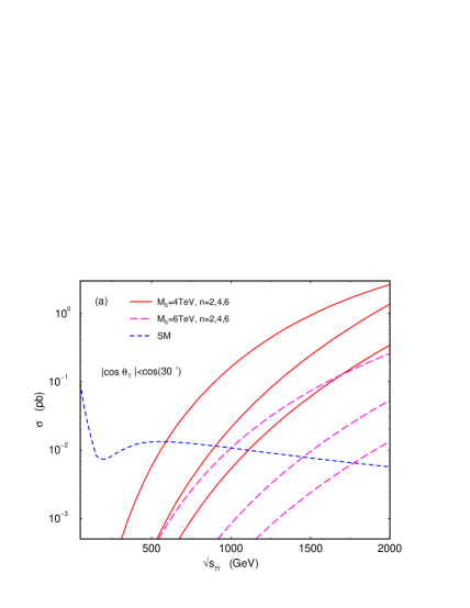
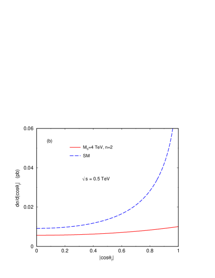
FIG. 1.: (a) The total cross sections and (b) the differential distribution $d\sigma/d|\cos\theta_{\gamma}|$ for $\gamma\gamma\to\gamma\gamma$ for the low scale gravity model and for the SM. A cut of $|\cos\theta_{\gamma}|<\cos 30^{\circ}$ is imposed.

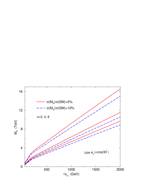
FIG. 2.: The sensitivity reach on $M_{S}$ versus $\sqrt{s_{\gamma\gamma}}$ using the process $\gamma\gamma\to\gamma\gamma$, by requiring the signal to be 5% or 10% of the SM prediction. A cut of $|\cos\theta_{\gamma}|<\cos 30^{\circ}$ is imposed.

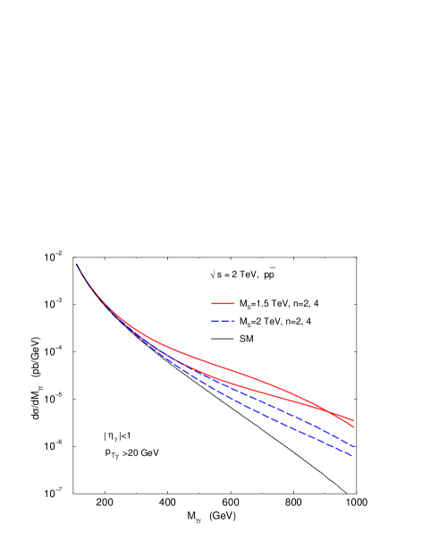
FIG. 3.: The differential distribution $d\sigma/dM_{\gamma\gamma}$ versus $M_{\gamma\gamma}$ for diphoton production at the 2 TeV Tevatron for the SM and for the low scale gravity with $M_{S}=1.5,\;2$ TeV and $n=2,4$. Cuts of $|\eta_{\gamma}|<1$ and $p_{T\gamma}>20$ GeV are imposed.

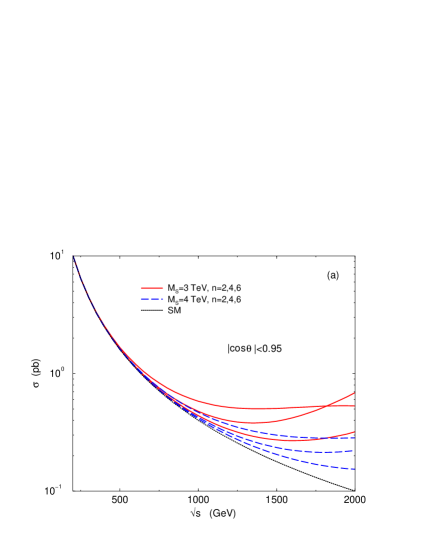
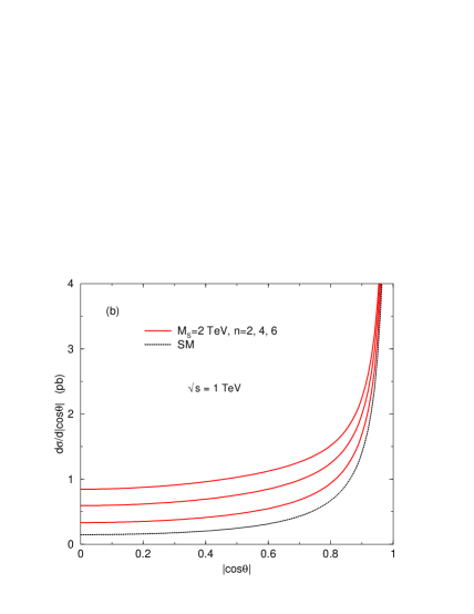
FIG. 4.: (a) The total cross section versus $\sqrt{s}$ and (b) the differential distribution $d\sigma/d|\cos\theta|$ for $e^{+}e^{-}\to\gamma\gamma$ for the SM and for the SM plus the new gravity interactions with $n=2,4,6$ and $M_{S}$ as shown. The $|\cos\theta|<0.95$ is imposed.

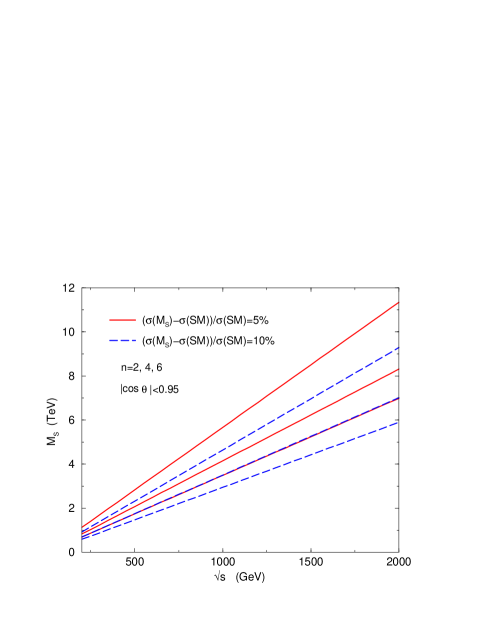
FIG. 5.: The sensitivity reach on $M_{S}$ versus $\sqrt{s}$ using the process $e^{+}e^{-}\to\gamma\gamma$, by requiring a 5% or 10% change from the SM prediction. A cut $|\cos\theta|<0.95$ is imposed.

REFERENCES

- [1] P. Horava and E. Witten, Nucl. Phys. B460, 506 (1996); ibid., B475, 94 (1996); E. Witten, ibid. B471, 135 (1996).
- [2] K. Dienes, E. Dudas, and T. Gherghetta, Phys. Lett. B436, 55 (1998); ibid., Nucl. Phys. B537, 47 (1999); C. Carone, WM-99-103, e-Print Archive: hep-ph/9902407; A. Delgado and M. Quiros, IEM-FT-189-99, e-Print Archive: hep-ph/9903400; P. Frampton and A. Rasin, IFP-769-UNC,e-Print Archive: hep-ph/9903479; T. Kobayashi, J. Kubo, M. Mondragon, and G. Zoupanos, HIP-1998-82-TH, e-Print Archive: hep-ph/9812221; Z. Kakushadze, HUTP-98-A073, e-Print Archive: hep-th/9811193;
- [3] See for example, P. Horava, Phys. Rev. D54, 7561 (1996); H. Nilles, M. Olechowski, M. Yamaguchi, Nucl. Phys. B530, 43 (1998); E. Mirabelli and M. Peskin, Phys. Rev. D58, 065002 (1998); L. Randall and R. Sundrum, e-Print archive: hep-th/9810155; A. Delgado, A. Pomarol, and M. Quiros, CERN-TH-98-393, e-Print Archive: hep-ph/9812489; I. Antoniadis, S. Dimopoulos, A. Pomarol, and M. Quiros, CERN-TH-98-332, e-Print Archive: hep-ph/9810410
- [4] I. Antoniadia, Phys. Lett. B246, 377 (1990); J. Lykken, Phys. Rev. D54, 3693 (1996); G. Shiu and S. Tye, Phys. Rev. D58, 106007 (1998); I. Antoniadis and C. Bachas, e-Print Archive hep-th/9812093.
- [5] N. Arkani-Hamed, S. Dimopoulos, G. Dvali, Phys. Lett. B429, 263 (1998); I. Antoniadis, N. Arkani-Hamed, S. Dimopoulos, and G. Dvali, Phys. Lett. B436, 257 (1998); N. Arkani-Hamed, S. Dimopoulos, G. Dvali, SLAC-PUB-7864, e-Print Archive: hep-ph/9807344; N. Arkani-Hamed, S. Dimopoulos, J. March-Russell, SLAC-PUB-7949, e-Print Archive: hep-th/9809124.
- [6] G. Giudice, R. Rattazzi, and J. Wells, Nucl. Phys. B544, 3 (1999).
- [7] S. Nussinov and R. Shrock, Phys. Rev. D59, 105002 (1999).
- [8] E. Mirabelli, M. Perelstein, and M. Peskin, Phys. Rev. Lett. 82, 2236 (1999).
- [9] T. Han, J. Lykken, and R. Zhang, e-Print Archive: hep-ph/9811350.
- [10] J. Hewett, SLAC-PUB-8001, e-Print Archive: hep-ph/98011356.
- [11] T. Rizzo, SLAC-PUB-8036, e-Print Archive: hep-ph/9901209.
- [12] P. Mathews, S. Raychaudhuri, and K. Sridhar, TIFR-TH-98-51, e-Print Archive: hep-ph/9812486.
- [13] P. Mathews, S. Raychaudhuri, and K. Sridhar, TIFR-TH-98-48, e-Print Archive: hep-ph/9811501.
- [14] Z. Berezhiani and G. Dvali, NYU-TH-10-98-06, e-Print Archive: hep-ph/9811378.
- [15] K. Agashe and N. Deshpande, e-Print Archive: hep-ph/9902263.
- [16] M. Graesser, e-Print Archive: hep-ph/9902310.
- [17] P. Nath and M. Yamagchi, e-Print Archive: hep-ph/9902323. M. Masip and A. Pomarol, e-Print Archive: hep-ph/9902467.
- [18] K. Cheung and W.-Y. Keung, e-Print Archive hep-ph/9903294.
- [19] T. Rizzo (SLAC). SLAC-PUB-8071, e-Print Archive: hep-ph/9903475.
- [20] D. Atwood, S. Bar-Shalom, and A. Soni, e-Print Archive: hep-ph/9903538.
- [21] C. Balázs, H.-J. He, W. Repko, C. Yuan, and D. Dicus, e-Print Archive: hep-ph/9904220.
- [22] A. Gupta, N. Mondal, and S. Raychaudhuri, e-Print Archive: hep-ph/9904234.
- [23] P. Mathews, S. Raychaudhuri, and K. Sridhar, e-Print Archive: hep-ph/9904232.
- [24] N. Arkani-Hamed, S. Dimopoulos, G. Dvali, and J. March-Russell, SLAC-PUB-8014, e-Print Archive: hep-ph/9811448; A. Faraggi and M. Pospelov, TPI-MINN-99-4, e-Print Archive: hep-ph/9901299; K. Dienes, E. Dudas, T. Gherghetta, CERN-TH-98-370, e-Print Archive: hep-ph/9811428; S. Cullen and M. Perelstein, SLAC-PUB-8084, e-Print Archive: hep-ph/9903422; C. Csaki, M. Graesser, and J. Terning, LBNL-42952, e-Print Archive: hep-ph/9903319; N. Arkani-Hamed, S. Dimopoulos, N. Kaloper, and J. March-Russell, SLAC-PUB-8068, e-Print Archive: hep-ph/9903224; A. Mazumdar, IMPERIAL-AST-99-2-2, e-Print Archive: hep-ph/9902381; G. Dvali and A. Smirnov, e-Print Archive: hep-ph/9904211; T. Banks, M. Dine, and A. Nelson, e-Print Archive: hep-th/9903019.
- [25] V. Costantinim B. de Tollis, and G. Pistoni, Nuovo Cim. A2, 733 (1971); G. Jikia and A. Tkabladze, Phys. Lett. B323, 453 (1994); G. Gounaris, P. Portfyriadis, and F. Renard, e-Print Archive: hep-ph/9902230.
- [26] D. Dicus and W. Repko, Phys. Rev. D48, 5106 (1993); A. Abbasabadi, A. Devoto, D. Dicus, and W. Repko Phys. Rev. D59, 013012 (1999).
- [27] D. Dicus and C. Kao, Phys. Rev. D49, 1265 (1994).
- [28] V. Telnov, I.F. Ginzburg, G.L. Kotkin, V.G. Serbo, and V.I. Telnov, Nucl. Inst. Meth. 205, 47 (1983).
- [29] “Search for High Mass Photon Pair in Collisions at TeV” submission by P. Wilson (CDF Coll.) to ICHEP’98; “Direct Photon Measurements at D0” submission by D0 Coll. to ICHEP’98.
- [30] ALEPH Coll., Phys. Lett. B429, 201 (1998); and contribution to the 1999 winter conference ALEPH 99-022; L3 Coll., Phys. Lett. B413, 159 (1997); and submission to ICHEP’98, L3 Internal Note 2269; DELPHI Coll., Phys. Lett. B433, 429 (1998); OPAL Coll., Phys. Lett. B438, 379 (1998); and OPAL Physics Note PN381.