UNICAL-TH 99/1

BITP-99-2E

DFPD 99/TH/6

March 1999

FIXED-ANGLE ELASTIC HADRON SCATTERING${}^{~{}\diamond}$

R. Fiore^1†, L. L. Jenkovszky^2‡, V. K. Magas^3∘, F. Paccanoni^4∗

¹ Dipartimento di Fisica, Università della Calabria,

Istituto Nazionale di Fisica Nucleare, Gruppo collegato di Cosenza

Arcavacata di Rende, I-87030 Cosenza, Italy

² Bogoliubov Institute for Theoretical Physics,

Academy of Sciences of the Ukraine

252143 Kiev, Ukraine

³ Section of Theoretical Physics (SENTEF)

Department of Physics, University of Bergen

Allegaten 55, 5007 Bergen, Norway

⁴ Dipartimento di Fisica, Università di Padova,

Istituto Nazionale di Fisica Nucleare, Sezione di Padova

via F. Marzolo 8, I-35131 Padova, Italy

The scattering amplitude in the dual model with Mandelstam analyticity and trajectory $\alpha(s)=\alpha_{0}-\gamma\ln\left[(1+\beta\sqrt{s_{0}-s})/(1+\beta\sqrt{s_{0}})\right]$ is studied in the limit $s,|t|\rightarrow\infty,\ s/t=const.$ By using the saddle point method, a series decomposition for the scattering amplitude is obtained, with the leading and two sub-leading terms calculated explicitly.

 

^⋄Work supported in part by the Research Council of Norway (programs for nuclear and particle physics, supercomputing, and free projects), in part by the Ministero italiano dell’Università e della Ricerca Scientifica e Tecnologica and in part by the INTAS grant 93-1867-extension $\begin{array}[]{ll}{}^{\dagger}\mbox{{\it email address:}}&\mbox{FIORE~{}@CS.INFN.IT}\end{array}$

$\begin{array}[]{ll}{}^{\ddagger}\mbox{{\it email address:}}&\mbox{JENK~{}@GLUK.APC.ORG}\end{array}$

$\begin{array}[]{ll}{}^{\circ}\mbox{{\it email address:}}&\mbox{MAGAS~{}@SENTEF2.FI.UIB.NO}\end{array}$

$\begin{array}[]{ll}{}^{\ast}\mbox{{\it email address:}}&\mbox{PACCANONI~{}@PADOVA.INFN.IT}\end{array}$

1 Introduction: Wide-angle scattering in QCD

Although attempts to apply perturbative QCD to wide-angle elastic hadron scatterings have been undertaken in a number of papers [1-10], explicit predictions have been available only for elastic processes involving external photons, such as $\gamma+\gamma\rightarrow$ hadrons, Compton scattering of hadrons, etc.

Predictions based on perturbative QCD rest on three premises: 1) hadronic interactions become weak at small invariant separation $r\ll\Lambda_{QCD}^{-1}$; 2) the perturbative expansion in $\alpha_{s}(Q)$ is well-defined; and 3) factorization, implying that all effects of collinear singularities, confinement, non-perturbative interactions and bound state dynamics can be isolated at large momentum transfer in terms of the (process independent) structure functions $G_{i/H}(x,Q),$ fragmentation functions $D_{H/i}(z,Q)$ or, in the case of exclusive processes, distribution amplitudes $\Phi_{H}(s_{i},Q).$ Consequently the hadronic scattering amplitude takes the form

$$A=\int\prod_{H}\phi_{H}(x_{i},Q)T(x_{i},p_{H};Q)[dx_{i}]~{},$$ (1)

where $\Phi(x_{i},Q)$ is a universal distribution amplitude which gives the probability amplitude for finding the valence $q\bar{q}$ or $qqq$ in the hadronic wave function collinear up to the scale $Q=\sqrt{s\over 2}$, and $T$ is the hard scattering amplitude for valence quark collisions.

The technical complication which has made particularly difficult to compute the behavior of hadron-hadron amplitudes is the possibility of multiple scatterings. The standard factorized form for the elastic scattering of hadrons $\{i\}$ is

$$A_{1}(s,t)=\int^{1}_{0}\prod_{i=1}^{4}[dx_{i}]\phi_{i}(x_{i})T(\{x_{i}\},s,t)~{},$$ (2)

where $x_{i}$ represents collectively the fractional momenta of hadron $i$ carried by its valence partons.

According to this concept, all of the partons collide in a small region of the space-time of typical dimension $Q^{-1}$. The relevant contribution to the amplitude behaves according to the dimensional counting [1, 2], i.e.

$$A_{1}(s,t)\sim({\mu^{2}\over s})^{n/2-2}f_{1}(s/t)$$ (3)

for $n$ partons participating in the hard scattering, $\mu$ representing hadronic mass scales, which make the amplitude dimensionless.

An extension of this ”single-scattering” scenario is the (double) ”independent- scattering” picture, due to P. Landshoff [8], in which two pairs of partons scatter independently off two scattering centers. According to this picture, the lowest order diagrams contribute with

$$A_{m}(s,t)\sim\biggl{(}{\mu^{2}\over s}\biggr{)}^{(n-m+1)/2-2}f_{m}(s/t)~{},$$ (4)

where $m$ is the number of independent scatterings. If so, the multiple scattering should dominate in the case of wide angle scattering.

A solution to this problem was pointed out in Refs. [5] and [11], where it was shown that the Sudakov logarithms associated with the rescattering diagrams do not cancel. In the leading logarithmic approximation they exponentiate to suppress the typical double scattering contribution by a factor

$$exp(-const\ln Q^{2}\ln(\ln Q^{2}))~{},$$

characteristic of the Sudakov suppression in QCD.

More quantitatively [12],

$$A_{2}\sim{1\over{Q^{4}}}\biggl{(}{Q\over\Lambda_{QCD}}\biggr{)}^{1-2c\ln(1/r)}\,,$$ (5)

where

$$r=2c/(1+2c)~{},~{}~{}~{}\ \ \ \ c=32/(33-2n_{f})~{},$$

and $n_{f}$ is the number of flavors. Interestingly, for $n_{f}=3$ the power turns out to be $Q^{-3.8},$ nearly the same as the dimensional counting power $Q^{-4}$ in the single-scattering scenario.

Higher order diagrams were calculated e.g. in Ref. [9], however soon it became evident that even the first order QCD correction involves an immense number of Feynman diagrams, so further attempts to go beyond the simple quark counting rule were abandoned.

It may be that perturbative QCD is not the relevant (or not the only physically interesting) expansion of the wide-angle scattering amplitude. Recent developments in M-branes (see e.g. Ref. citepolchinski) may open new prospects in the realization of a hypothetical duality between small and large distances (or, equivalently, large- and small-angle scattering). The search for a relevant expansion parameter is of crucial importance on this way.

In this paper we are solving an ”inverse problem”: we use the known explicit expression of the dual amplitude with Mandelstam analyticity (DAMA), that has correct wide angle scaling behavior. By identifying it with that resulting from the quark counting rules, we then calculate two sub-leading terms in the expansion of the known full dual amplitude and study the behavior of the resulting series.

2 Wide angle behavior of the dual amplitude with Mandelstam analyticity

Wide-angle scaling behavior within the $S-$matrix approach was discussed in Ref. [13], where by means of a logarithmic Regge trajectory an interpolation from the “soft“ Regge behavior to the “hard“ scaling regime was suggested. The motivation of the logarithmic trajectory came from earlier papers [14], where a class of dual models requiring a logarithmic trajectory was suggested.

The logarithmic asymptotic behavior of the trajectory and the large angle scaling behavior are uniquely related also in a different class of dual models, called dual amplitudes with Mandelstam analytics (DAMA) [15, 16]. The link between this class of models in the scaling limit and the parton model in the infinite momentum frame was studied in Ref. [17]. In all those papers only the leading asymptotic ($s,|t|\rightarrow\infty,\ s/t=const$) term was treated. The results of different approaches vary in such details as the form of the scaling violation (normally, logarithmic), the form of the angular dependence $f(\theta)$ and the way active quarks are counted.

In this paper we calculate the sub-leading terms in the pre-asymptotic (larger $s$ and $|t|$) behavior of DAMA. Since the model is realistic enough in the sense that it satisfies the general requirements of the theory (see Refs. [15, 16]), we believe that our result is universal and thus it may be used as a guide e. g. in QCD calculations.

Apart from the leading term, we have explicitly calculated two more sub-leading terms. Our technique allows further calculations of still higher orders, but the obtained first three terms of the series already show a regular trend that may be interpreted as the expansion in the running coupling constant $g(s)\sim 1/\ln s,$ valid at large $s$ and $|t|$. This situation takes place for anyone trajectory with the logarithmic asymptotic.

The aim of the present paper is two-fold. First, by identifying the leading term of the asymptotic (wide-angle) expansion of DAMA with that derived from perturbative QCD [5] we tentatively assume that the DAMA in the wide angle asymptotic region is equivalent to the asymptotically free regime in QCD. With this identification in mind, we calculate within DAMA corrections to the leading term in the hope that their form may give some insight into the relevant corrections in perturbative QCD that are known to be very complicated.

Clearly, the above identity has the chance to be true only in the vicinity of the wide angle region (small distances), where perturbative calculations are assumed to be still valid.

The second aspect is purely phenomenological. Since, however, the experimental situation in the wide-angle region did not change for almost two decades, we are left with the earlier fits to the data.

Let us now calculate the “perturbative“ expansion of DAMA. We write the elastic scattering amplitude for spinless particles in the following symmetric form [16]:

$$A(s,t,u)=C(s-u)[D(s,t)-D(u,t)]~{},$$ (6)

where $C$ is a constant and

$$D(s,t)=\int\limits_{0}^{1}dx\left(\frac{x}{g}\right)^{-\alpha(s^{\prime})}\left(\frac{1-x}{g}\right)^{-\alpha(t^{\prime})}~{}.$$ (7)

Here $s^{\prime}=s(1-x),\ \ \ t^{\prime}=tx$ and $g$ is a dimensionless parameter, $g>1$. Only one, leading trajectory was included and it was chosen in a simple, but representative form:

$$\alpha(s)=\alpha_{0}-\gamma\ln\left(\frac{1+\beta\sqrt{s_{0}-s}}{1+\beta\sqrt{s_{0}}}\right)~{},$$ (8)

that account both for the threshold and the asymptotic behavior and is nearly linear for very small $|s|,|s|<<s_{0}\,.$ For simplicity we have included only the leading trajectories in both channels: the Pomeron trajectory in the $t$-channel and the exotic trajectory in the $s$-channel. While the parameters of the Pomeron trajectory are well known, only a little is known about the exotic trajectory. Fortunately, this has no substantial effect on our results, since our goal is the functional form of the series and its individual terms rather than fits to the data. Given the scarcity of the data and the freedom available in the model, the wide-angle behavior of DAMA cannot be determined completely.

Let us consider the asymptotic behavior of Eq. (7) in the limit $s,\left|t\right|\rightarrow\infty,\ s/t=const.$ For the Regge trajectories we have

$$\alpha(s)=\alpha(0)-\frac{\gamma}{2}\ln\delta^{2}+i\pi\frac{\gamma}{2}-\frac{\gamma}{2}\ln s=-a-\lambda~{},$$ (9)

$$\alpha(t)=\alpha(0)-\frac{\gamma}{2}\ln\delta^{2}-\frac{\gamma}{2}\ln\left(-\frac{t}{s}\right)-\frac{\gamma}{2}\ln s=-b-\lambda~{},$$ (10)

with

$$a=-\alpha(0)+\frac{\gamma}{2}\ln\delta^{2}-i\pi\frac{\gamma}{2}~{},~{}~{}~{}~{}b=-\alpha(0)+\frac{\gamma}{2}\ln\delta^{2}+\frac{\gamma}{2}\ln(-\frac{t}{s})~{},$$

$$\delta=\frac{\beta\sqrt{s_{0}}}{1+\beta\sqrt{s_{0}}}~{},~{}~{}~{}~{}~{}~{}\lambda=\frac{\gamma}{2}\ln s~{}.$$ (11)

From here on, $s,t,u$ will be dimensionless variables, measured in units of $s_{0}$.

In this domain the saddle point method can be used to calculate the integral in Eq. (7) [21]. To do this we can rewrite Eq. (7) in the following form

$$D(s,t)=(2g)^{-a-b-2\lambda}g^{\gamma\ln 2}{1\over 2}\int\limits_{-1}^{1}g(u)~{}e^{\lambda f(u)}du~{},$$ (12)

where we have changed the variable $x$ to $u$, $x=(1-u)/2$, and introduced new functions:

$$g(u)=(1-u)^{\tilde{a}}(1+u)^{\tilde{b}}e^{\gamma\ln{\frac{1-u}{2}}\ln{\frac{1+u}{2}}}~{},$$ (13)

$$f(u)=\ln(1-u^{2})~{},$$ (14)

$$\tilde{a}=a-\frac{\gamma}{2}\ln g~{},\ \ \ \ \ \tilde{b}=b-\frac{\gamma}{2}\ln g~{}.$$ (15)

We see now that $f(u)$ has a sharp maximum at the saddle point $u_{0}=0$.

We quote the explicit expression for the saddle point expansion in the Appendix A. Using formulas from this Appendix we obtain the power series for $D(s,t)$ in Appendix B. It reads

$$D(s,t)\approx\frac{A_{1}s^{-\gamma\ln 2g}}{\sqrt{\gamma\ln s}}\left(-\frac{t}{s}\right)^{-\frac{\gamma}{2}\ln 2g}\left\{1+\frac{h_{1}(\tilde{a},\tilde{b})}{\gamma\ln s}+\frac{h_{2}(\tilde{a},\tilde{b})}{(\gamma\ln s)^{2}}\right\}~{},$$ (16)

where $A_{1},\ h_{1},\ h_{2}$ are given by the expressions (B.5, B.8, B.9). The expression for $D(u,t)$ can be calculated in a similar way (see Eq. (B.10) in Appendix B).

In the kinematical region $s,\left|t\right|\rightarrow\infty,\ t/s=const$ we can use the substitutions

$$t\approx-s\cdot\sin^{2}\left(\theta/2\right)~{},~{}~{}~{}~{}~{}~{}u\approx-s\cdot\cos^{2}\left(\theta/2\right)~{}.$$ (17)

Substituting the results for $D(s,t)$ and $D(u,t)$ into Eq. (6) and changing the variables we get the expression for the full amplitude as a function of the $s$ and $\theta$ variables (see Eq. (B.14) in Appendix B):

$$A(s,\theta)\approx\frac{CAs^{-N}}{\sqrt{\gamma\ln s}}f(\theta)I(s,\theta)~{},$$ (18)

where $A,\ N,\ f(\theta),\ I(s,\theta)$ are given by the expressions (B.13, B.15 - B.17).

To summarize, we have expanded the wide-angle scattering amplitude in a power series of $1/\ln{s}$ and have evaluated explicitly the coefficients of the first two terms (beyond the leading one).

3 Comparison with the data and discussion of the results

New experimental data on wide-angle scatterings are not likely to appear any more because of the simple reason that as energy increases more particles tend to fly in the forward direction and there is no chance to detect e.g. the proton-proton differential cross section at $90^{\circ}$ for, say, $\sqrt{s}>10\ GeV$. “Wide angles”, of course, extend beyond $90^{\circ}$. Still the complication due to the huge number of Born diagrams contributing to large angle exclusive reactions [5], overwhelming the contribution due to the Landshoff pinch singularity [8], will remain for long topical in this field. We use the data given in the compilation of [20] to fix the scale. The errors, quoted in the original papers (see Ref. [20] and references therein), are typically about 10 overall normalization factor, the ”quark counting power” in the cross section being set equal to $N=4$ in the case of proton-proton cross section, in agreement with the data [20, 5] (see Fig. 1).

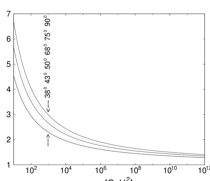
Figure 1: Cross section $\frac{d\sigma}{dt}$ for pp $\rightarrow$ pp scattering at various center of mass scattering angles. Both axes are in logarithmic scale. Stars denote the experimental points from Ref. [20]. The straight lines correspond to a falloff of $\sim 1/s^{10}$. They are calculated according to the power series for the scattering amplitude, discussed above ($\frac{d\sigma}{dt}=\frac{4\pi}{(ss_{0})^{2}}|A(s,\theta)|^{2}$), with the following set of parameters: $\alpha_{0}=1$, $N=4,\ \gamma=2.84\ (g=2.9),$ $\beta=0.05\ GeV^{-1}$, $C=2.7\cdot 10^{-14}GeV^{-2}$ and $s_{0}=4m_{\pi}^{2}$.

Our main goal is the behavior of the scaling-violating corrections to the leading term obeying quark counting rules. Fig. 2 shows the relative contribution of these terms. We draw the correction power series:

$$J(s,\theta)=|I(s,\theta)|^{2}\approx 1+2\frac{Re(f_{1}(\theta)/Z(\theta))}{\gamma\ln s}+2\frac{Re(f_{2}(\theta)/Z(\theta))}{(\gamma\ln s)^{2}}+\frac{|f_{1}(\theta)/Z(\theta)|^{2}}{(\gamma\ln s)^{2}}$$

$$+O({1\over\lambda^{3}})~{},$$ (19)

where $f_{1}(\theta),~{}f_{2}(\theta),~{}Z(\theta)$ are given by expressions (B.18 - B.20). We can see that the corrections are quite large for small $s$, especially for angles close to $90^{0}$. That is not a surprise, since the lowest order of our expansion is valid for large $s$ ($\gamma\ln s/2>>1$). In the experimental energy interval the corrections give factor $4-6$ to the cross sections and should not be neglected. This was missed in the references [15, 16]. Moreover we find that the corrections are very sensitive to variations of $\beta$ and $\gamma$.

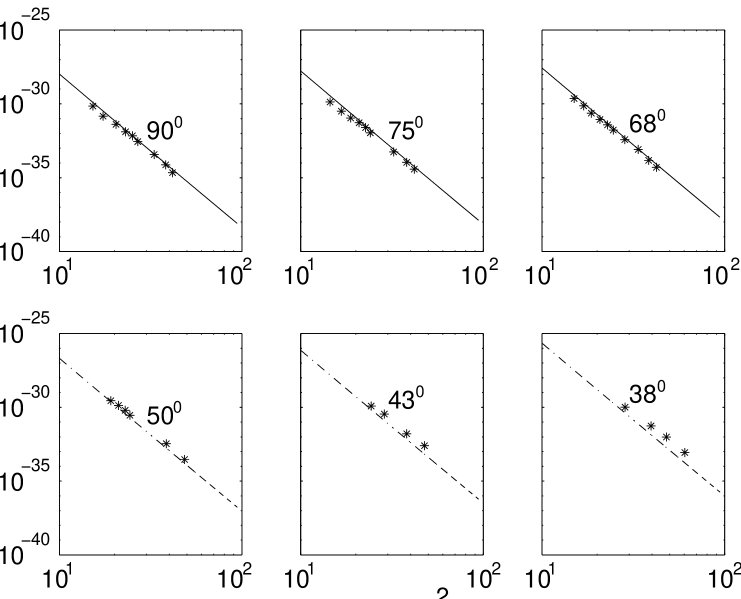
Figure 2: The corrections $J(s,\theta)$, given by Eq. (19), to the differential cross section $\frac{d\sigma}{dt}$ for pp $\rightarrow$ pp scattering . We have used the same values of parameters as in Fig. 1: $\alpha_{0}=1$, $N=4,\ \gamma=2.84\ (g=2.9),$ $\beta=0.05\ GeV^{-1}$ and $s_{0}=4m_{\pi}^{2}$, coming from the comparison with the data.

Acknowledgment V.K. Magas is thankful for the hospitality extended to him by the Bogolyubov Institute for Theoretical Physics in Kiev where part of this work was done.

Appendix A : Coefficients in the saddle point method

In this Appendix we present the explicit expression for the saddle point expansion from Ref. [19]. Here $f^{(k)}(u_{0})\equiv f_{k}~{},~{}~{}~{}g^{(k)}(u_{0})\equiv g_{k}~{}.$

$$\int\limits_{-1}^{1}g(u)~{}e^{\lambda f(u)}du=e^{\lambda f(u_{0})}\sqrt{\frac{\pi}{\lambda}}\left[a_{0}+{a_{1}\over\lambda}+{a_{2}\over\lambda^{2}}+O(\frac{1}{\lambda^{3}})\right]~{}.$$ (A.1)

where

$$a_{0}=\psi_{1}g_{0}~{},~{}~{}~{}a_{1}={1\over 4}\left[g_{2}\psi_{1}^{3}+3g_{1}\psi_{1}\psi_{2}+g_{0}\psi_{3}\right]~{},$$

$$a_{2}={1\over 32}\left[g_{4}\psi_{1}^{5}+10g_{3}\psi_{1}^{3}\psi_{2}+10g_{2}\psi_{1}^{2}\psi_{3}+15g_{2}\psi_{2}^{2}\psi_{1}+5g_{1}\psi_{4}\psi_{1}+10g_{1}\psi_{3}\psi_{2}+g_{0}\psi_{5}\right]~{}.$$ (A.2)

$$\psi_{1}=\sqrt{\frac{2}{-f_{2}}}~{},~{}~{}~{}\psi_{2}=-{1\over 3}f_{3}f_{2}^{-1}\psi_{1}^{2}~{},~{}~{}~{}\psi_{3}=\left[-{1\over 4}f_{4}f_{2}^{-1}+{5\over 12}f_{3}^{2}f_{2}^{-2}\right]\psi_{1}^{3}~{},$$

$$\psi_{4}=\left[-{1\over 5}f_{5}f_{2}^{-1}+f_{4}f_{3}f_{2}^{-2}-{8\over 9}f_{3}^{3}f_{2}^{-3}\right]\psi_{1}^{4}~{},$$

$$\psi_{5}=\left[-{1\over 6}f_{6}f_{2}^{-1}+{7\over 6}f_{5}f_{3}f_{2}^{-2}+{35\over 48}f_{4}^{2}f_{2}^{-2}+{385\over 144}f_{3}^{4}f_{2}^{-4}-{35\over 8}f_{4}f_{3}^{2}f_{2}^{-3}\right]\psi_{1}^{5}~{}.$$ (A.3)

Appendix B : Calculations of the scattering amplitude

Using the definitions of functions $g(u)$, $f(u)$ (13, 14) we obtain

$$f_{2}=-2~{},~{}~{}~{}f_{3}=0~{},~{}~{}~{}f_{4}=-12~{},~{}~{}~{}f_{5}=0~{},~{}~{}~{}f_{6}=-240~{},$$ (B.1)

$$g_{0}=e^{\gamma\ln^{2}2}~{},~{}~{}~{}g_{2}=g_{0}\left[(\tilde{a}-\tilde{b})^{2}-(\tilde{a}+\tilde{b})+2\gamma(\ln 2-1)\right]~{},$$

$$g_{4}=g_{0}\left[\tilde{a}(\tilde{a}-1)(\tilde{a}-2)(\tilde{a}-3)-4\tilde{a}(\tilde{a}-1)(\tilde{a}-2)\tilde{b}+6\tilde{a}(\tilde{a}-1)\tilde{b}(\tilde{b}-1)-4\tilde{a}\tilde{b}(\tilde{b}-1)(\tilde{b}-2)+\right.$$

$$\ \left.\tilde{b}(\tilde{b}-1)(\tilde{b}-2)(\tilde{b}-3)+12\gamma\left((\tilde{a}-\tilde{b})^{2}-(\tilde{a}+\tilde{b})\right)(\ln 2-1)+12\gamma^{2}(\ln 2-1)^{2}\right.$$

$$\left.+2\gamma(6\ln 2-5)\right]~{}.$$ (B.2)

From Eq. (A.3, B.1) we get

$$\psi_{1}=1~{},~{}~{}~{}\psi_{2}=0~{},~{}~{}~{}\psi_{3}=-{3\over 2}~{},~{}~{}~{}\psi_{4}=0~{},~{}~{}~{}\psi_{5}={25\over 4}~{}.$$ (B.3)

Finally we get

$$D(s,t)\approx\frac{A_{1}s^{-N_{1}}}{\sqrt{\gamma\ln s}}\left(-\frac{t}{s}\right)^{-\frac{\gamma}{2}\ln 2g}I(\tilde{a},\tilde{b},s)~{},$$ (B.4)

where

$$A_{1}=(2g)^{2\alpha_{0}-\gamma\ln\delta^{2}+\gamma\ln 2+i\pi\gamma/2}\sqrt{\frac{\pi}{2}}~{},$$ (B.5)

$$N_{1}=\gamma\ln 2g~{},$$ (B.6)

$$I(\tilde{a},\tilde{b},s)=\left\{1+\frac{h_{1}(\tilde{a},\tilde{b})}{\gamma\ln s}+\frac{h_{2}(\tilde{a},\tilde{b})}{(\gamma\ln s)^{2}}\right\}~{},$$ (B.7)

Coefficients $h_{1}(\tilde{a},\tilde{b}),~{}h_{2}(\tilde{a},\tilde{b})$ are calculated from (A.2, B.2, B.3)

$$h_{1}(\tilde{a},\tilde{b})=-\left(\frac{3}{4}-\frac{g_{2}}{2g_{0}}\right)~{},$$ (B.8)

$$h_{2}(\tilde{a},\tilde{b})=\left({25\over 32}+\frac{g_{4}}{8g_{0}}-\frac{15g_{2}}{8g_{0}}\right)~{}.$$ (B.9)

The expression for $D(u,t)$ can be calculated in a similar way. It turns out to be

$$D(u,t)\approx\frac{A_{2}s^{-N_{1}}}{\sqrt{\gamma\ln s}}\left(\frac{ut}{s^{2}}\right)^{-\frac{\gamma}{2}\ln 2g}I(\tilde{c},\tilde{b},s)~{},$$ (B.10)

where

$$A_{2}=(2g)^{2\alpha_{0}-\gamma\ln\delta^{2}+\gamma\ln 2}\sqrt{\frac{\pi}{2}}~{},$$

$$\tilde{c}=c-{\gamma\over 2}\ln g=-\alpha(0)+\frac{\gamma}{2}\ln\delta^{2}+\frac{\gamma}{2}\ln\left(-\frac{u}{s}\right)-{\gamma\over 2}\ln g~{}.$$ (B.11)

Substituting Eqs. (B.4) and (B.10) into Eq. (6) we get the expression for the full amplitude:

$$A(s,t,u)\approx C\frac{A}{s_{0}}\frac{s^{-N_{1}}}{\sqrt{\gamma\ln s}}\ (s-u)s_{0}\left\{(2g)^{\frac{i\pi\gamma}{2}}\left(-\frac{t}{s}\right)^{-\frac{\gamma}{2}\ln 2g}I(\tilde{a},\tilde{b},s)\right.$$

$$\left.\hfill-\left(\frac{tu}{s^{2}}\right)^{-\frac{\gamma}{2}\ln 2g}I(\tilde{c},\tilde{b},s)\right\}\hfill~{},$$ (B.12)

where

$$A=(2g)^{2\alpha(0)-\gamma\ln\delta^{2}+\gamma\ln 2}\sqrt{\frac{\pi}{2}}s_{0}~{},$$ (B.13)

In the kinematical region $s,\left|t\right|\rightarrow\infty,\ t/s=const$ we can use the substitutions (17). So, the expression for the scattering amplitude as a function of $s$ and $\theta$ appears to be

$$A(s,\theta)\approx C\frac{As^{-N}}{\sqrt{\gamma\ln s}}f(\theta)I(s,\theta)~{},$$ (B.14)

where

$$N=N_{1}-1=\gamma\ln 2g-1~{},$$ (B.15)

$$f(\theta)=\left(1+\cos^{2}\frac{\theta}{2}\right)\left(\sin\frac{\theta}{2}\right)^{-\gamma\ln 2g}Z(\theta)~{},$$ (B.16)

$$I(s,\theta)=1+\frac{f_{1}(\theta)}{Z(\theta)\gamma\ln s}+\frac{f_{2}(\theta)}{Z(\theta)(\gamma\ln s)^{2}}~{},$$ (B.17)

$$f_{1}(\theta)=h_{1}(\tilde{a},\tilde{b})(2g)^{\frac{i\pi\gamma}{2}}-h_{1}(\tilde{c},\tilde{b})(2g)^{-\gamma\ln\cos\frac{\theta}{2}}~{},$$ (B.18)

$$f_{2}(\theta)=h_{2}(\tilde{a},\tilde{b})(2g)^{\frac{i\pi\gamma}{2}}-h_{2}(\tilde{c},\tilde{b})(2g)^{-\gamma\ln\cos\frac{\theta}{2}}~{},$$ (B.19)

$$Z\left(\theta\right)=(2g)^{\frac{i\pi\gamma}{2}}-(2g)^{-\gamma\ln\cos\frac{\theta}{2}}~{},$$ (B.20)

$$\tilde{b}=-\alpha(0)+\frac{\gamma}{2}\ln\delta^{2}+\frac{\gamma}{2}\ln\left(\sin^{2}\left(\frac{\theta}{2}\right)\right)-{\gamma\over 2}\ln g~{},$$ (B.21)

$$\tilde{c}=-\alpha(0)+\frac{\gamma}{2}\ln\delta^{2}+\frac{\gamma}{2}\ln\left(\cos^{2}\left(\frac{\theta}{2}\right)\right)-{\gamma\over 2}\ln g~{}.$$ (B.22)

References

• [1] S. J. Brodsky and G. R. Farrar Phys. Rev. Lett. 31 (1973) 1153.
• [2] V. A. Matveev and A. N. Tavkhelidze, R. M. Muradyan Letter Nuovo Cimento 7 (1973) 179.
• [3] S. J. Brodsky and G. R. Farrar Phys. Rev. D 11 (1974) 1309.
• [4] A. V. Efremov and S. J. Brodsky Theo. and Math. Phys. 42 (1980) 97.
• [5] S. J. Brodsky and G. P. Lepage Phys. Rev. D. 22 (1980) 2157; J. C. Collins, D. E. Soper and G. Sterman, Perturbative quantum chromodynamics, ed. by A. H. Muller, World Scientific, Singapore, 1989.
• [6] A. Duncan and A. H. Mueller Phys. Rev. D 21 (1980) 1636.
• [7] N. Isgur and C. H. Llewellyn Smith Nucl. Phys. B 317 (1989) 526.
• [8] P. V. Landshoff Phys. Rev. D 10 (1974) 1024.
• [9] G. R. Farrar, G. Sterman and H. Zhang Phys. Rev. Lett. 62 (1989) 2229.
• [10] J. Botts and G. Sterman Nucl. Phys. B (Proc. Suppl.) 12 (1990) 53.
• [11] P. V. Landshoff and D. J. Pritchard Z. fur Phys. C 6 (1981) 69.
• [12] A. H. Mueller Phys. Rep. 73 (1981) 237.
• [13] D. D. Coon et al. Phys. Rev. D. 18 (1978) 1451.
• [14] M. Arik Phys. Rev. D. 11 (1975) 602.
• [15] L. L. Jenkovszky and Z. E. Chikovani Yadernaya fizika 30 (1979) 531.
• [16] A. I. Bugrij, Z. E. Chikovani and L. L. Jenkovszky Z. Phys. C 4 (1980) 45.
• [17] M. J. Schmidt Phys. Lett. B 43 (1973) 417.
• [18] H. Kluberg and J. Zuber Phys. Rev. D 12 (1975) 467; 482; 3159.
• [19] M. V. Fedoryuk Asimptotika: ryady i integraly - M.:Nauka, 1987, in Russian.
• [20] P. V. Landshoff and J. C. Polkinghorne Phys. Lett. B. 44 (1973) 293.
• [21] V. Magas Ukrainsky Fizichesky Journal, in press.
• [22] J. Polchinski Rev. Mod. Phys. 68 (1996) 1245.