The angular distribution of the reaction $\bar{\nu}_{e}+p\rightarrow e^{+}+n$

Abstract

The reaction $\bar{\nu}_{e}+p\rightarrow e^{+}+n$ is very important for low-energy ($E_{\nu}\lesssim 60$ MeV) antineutrino experiments. In this paper we calculate the positron angular distribution, which at low energies is slightly backward. We show that weak magnetism and recoil corrections have a large effect on the angular distribution, making it isotropic at about 15 MeV and slightly forward at higher energies. We also show that the behavior of the cross section and the angular distribution can be well-understood analytically for $E_{\nu}\lesssim 60$ MeV by calculating to ${\cal O}(1/M)$, where $M$ is the nucleon mass. The correct angular distribution is useful for separating $\bar{\nu}_{e}+p\rightarrow e^{+}+n$ events from other reactions and detector backgrounds, as well as for possible localization of the source (e.g., a supernova) direction. We comment on how similar corrections appear for the lepton angular distributions in the deuteron breakup reactions $\bar{\nu}_{e}+d\rightarrow e^{+}+n+n$ and $\nu_{e}+d\rightarrow e^{-}+p+p$. Finally, in the reaction $\bar{\nu}_{e}+p\rightarrow e^{+}+n$, the angular distribution of the outgoing neutrons is strongly forward-peaked, leading to a measurable separation in positron and neutron detection points, also potentially useful for rejecting backgrounds or locating the source direction.

]

I Introduction

Inverse neutron beta decay, $\bar{\nu}_{e}+p\rightarrow e^{+}+n$, is the reaction of choice for the detection of reactor antineutrinos, crucial to neutrino oscillation searches. It is also, by far, the reaction giving the largest yield for the detection of supernova neutrinos. The LSND [1] and KARMEN [2] experiments use $\bar{\nu}_{\mu}$ antineutrinos from $\mu^{+}$ decay at rest to search for the oscillation appearance of $\bar{\nu}_{e}$ events, detected by this reaction. There are also searches for $\bar{\nu}_{e}$ antineutrinos from the Sun.

In many of these applications, in particular those based on detection by Čerenkov radiation, one can determine the direction of the outgoing positron. It is therefore of interest to consider the angular correlation between the incoming antineutrino and outgoing positron directions, and its energy dependence for $E_{\nu}\lesssim 60$ MeV, relevant for the above studies. If the source direction is known, the angular correlation can be used to help separate these events from other reactions or detector backgrounds. If the source direction is unknown, as possibly for a Galactic supernova, then the observed angular distribution may help to locate the source.

For low antineutrino energies, the positron angular distribution is well-described by the form

$$\frac{{\rm d}\sigma}{{\rm d}\cos\theta}\simeq 1+v_{e}a(E_{\nu})\cos\theta\,,$$ (1)

where $\theta$ is the angle between the antineutrino and positron directions in the laboratory (where the proton target is assumed to be at rest) and $v_{e}$ is the positron velocity in $c=1$ units. At higher energies, terms proportional to higher powers of $\cos\theta$ appear, and at the highest energies, all reaction products are strongly forward simply by kinematics. It is convenient to describe the angular distribution by the average cosine, weighted by the differential cross section, since that is always well-defined. In the limit that Eq. (1) holds,

$$\langle\cos\theta\rangle=\frac{1}{3}v_{e}a(E_{\nu})\,,$$ (2)

where the $E_{\nu}$-dependence of $\langle\cos\theta\rangle$ is suppressed in the notation here and below. Except near threshold, where $v_{e}$ becomes very small (but nonzero in the lab), the $v_{e}$ factor is nearly unity and can be ignored.

In the limit where the nucleon mass is taken to be infinite, i.e., zeroth order in $1/M$, the asymmetry coefficient $a$ is independent of $E_{\nu}$ and would be the same for $\bar{\nu}_{e}+p\rightarrow e^{+}+n$ and $\nu_{e}+n\rightarrow e^{-}+p$. (Since there are no free neutron targets, the latter cannot be directly observed. We return to this point below in discussing neutrino and antineutrino reactions with deuterons.) Then $a^{(0)}$ is given simply by the competition of the non-spin-flip (Fermi) and spin-flip (Gamow-Teller) contributions, and is

$$a^{(0)}=\frac{f^{2}-g^{2}}{f^{2}+3g^{2}}\simeq-0.10\,,$$ (3)

and thus the angular distribution of the positrons is weakly backward. We have defined the vector and axial-vector coupling constants by $f=1$, $g=1.26$.

In the following we will consider how $\langle\cos\theta\rangle$ is modified when weak magnetism and recoil corrections of ${\cal O}(1/M)$ are kept. The effect of these terms on the total cross section was calculated in Refs. [3, 4] (see also Ref. [5]), where it was found that they, in particular the weak magnetism, reduce the cross section by a noticeable amount. In this paper, we will show that the positron angular distribution is changed even more, including the sign of $\langle\cos\theta\rangle$. The effect is so large in part because of the accidental near-cancelation in $a^{(0)}$.

The general form of the differential cross section, valid to all orders in $1/M$ but neglecting the threshold effects (and hence only valid for energies far above threshold), is well-known [6]. For the relevant energies $E_{\nu}\lesssim 60$ MeV, it is instructive and sufficient to consider in detail just the terms of first order in $1/M$. Here and below, $1/M$ will be taken to refer to all terms of that form, with $E_{\nu}/M$ being dominant among them. Moreover, using these results, we show how to extend the formula of Ref. [6] to low energies, so that it merges smoothly with the correct expression near threshold.

II The positron angular distribution

A Differential cross section: expansion in powers of $1/M$

We begin with the matrix element of the form

$${\cal M} = \frac{G_{F}\cos\theta_{C}}{\sqrt{2}}\left[\bar{u}_{n}\left(\gamma_{\mu}f-\gamma_{\mu}\gamma_{5}g-\frac{if_{2}}{2M}\sigma_{\mu\nu}q^{\nu}\right)u_{p}\right]$$ (4)

$$\times \left[\bar{v}_{\bar{\nu}}\gamma^{\mu}(1-\gamma_{5})v_{e}\right]\,,$$ (5)

where $f$ and $g$ are given above, the anomalous nucleon isovector magnetic moment is defined with $f_{2}=\mu_{p}-\mu_{n}=3.706$, and $\cos\theta_{C}=0.974$. In the most general case, the coupling constants are replaced with form factors that vary with $q^{2}$; we neglect this variation as it is ${\cal O}(E_{\nu}^{2}/M^{2})$. The four-momentum transfer $q^{2}$ is related to the laboratory scattering angle $\theta$, which in turn is related to the outgoing positron energy $E_{e}$ (again in the laboratory) by the relations

$$q^{2} = m_{e}^{2}-2E_{\nu}E_{e}(1-v_{e}\cos\theta)$$ (6)

$$= (M_{n}^{2}-M_{p}^{2})-2M_{p}(E_{\nu}-E_{e})\,.$$ (7)

Some other useful kinematic relations are given in the Appendix. We can now use the standard rules and evaluate the differential cross section accurate to a given order in $1/M$.

At zeroth order in $1/M$, the positron energy is

$$E_{e}^{(0)}=E_{\nu}-\Delta,$$ (8)

where $\Delta=M_{n}-M_{p}$. At each order in $1/M$, we define the positron momentum $p_{e}=\sqrt{E_{e}^{2}-m_{e}^{2}}$ and the velocity $v_{e}=p_{e}/E_{e}$. The differential cross section at this order is

$$\left(\frac{{\rm d}\sigma}{{\rm dcos}\theta}\right)^{(0)}$$ (9)

$$= \frac{\sigma_{0}}{2}\left[(f^{2}+3g^{2})+(f^{2}-g^{2})v_{e}^{(0)}\cos\theta\right]E_{e}^{(0)}p_{e}^{(0)}\,.$$ (10)

The normalizing constant $\sigma_{0}$, including the energy-independent inner radiative corrections, is

$$\sigma_{0}=\frac{G_{F}^{2}\cos^{2}\theta_{C}}{\pi}\;(1+\Delta^{R}_{inner})\,,$$ (11)

where $\Delta^{R}_{inner}\simeq 0.024$ [7]. This gives the standard result for the total cross section,

$$\sigma^{(0)}_{tot} = \sigma_{0}\;(f^{2}+3g^{2})\;E_{e}^{(0)}p_{e}^{(0)}$$ (12)

$$= 0.0952\left(\frac{E_{e}^{(0)}p_{e}^{(0)}}{1{\rm\ MeV}^{2}}\right)\times 10^{-42}{\rm\ cm}^{2}\,.$$ (13)

The energy-independent inner radiative corrections affect the neutron beta decay rate in the same way, and hence the total cross section can also be written

$$\sigma^{(0)}_{tot}=\frac{2\pi^{2}/m_{e}^{5}}{f^{R}_{p.s.}\tau_{n}}\;E_{e}^{(0)}p_{e}^{(0)}\,,$$ (14)

where $\tau_{n}$ is the measured neutron lifetime and $f^{R}_{p.s.}=1.7152$ is the phase space factor, including the Coulomb, weak magnetism, recoil, and outer radiative corrections, but not the inner radiative corrections [8]. The cross section normalization was measured in Ref. [9] and found to be in agreement with the expectation from the neutron lifetime at the 3% level. The (small) energy-dependent outer radiative corrections to $\sigma_{tot}$ are given in Refs. [3, 4]. The outer radiative corrections to $\langle\cos\theta\rangle$ should largely cancel in the ratio of the cross section weighted with $\cos\theta$ to the cross section itself, and so are not considered further here.

At first order in $1/M$, the positron energy depends upon the scattering angle and is

$$E_{e}^{(1)}=E_{e}^{(0)}\left[1-\frac{E_{\nu}}{M}(1-v_{e}^{(0)}\cos\theta)\right]-\frac{y^{2}}{M}\,,$$ (15)

where $y^{2}=(\Delta^{2}-m_{e}^{2})/2$. In factors of the form $1/M$, we use the average nucleon mass; using $1/M$ versus $1/M_{p}$ leads to an ignorable difference of ${\cal O}(1/M^{2})$. The differential cross section at this order (after a lot of tedious algebra) is

$$\left(\frac{{\rm d}\sigma}{{\rm dcos}\theta}\right)^{(1)}$$ (16)

$$= \frac{\sigma_{0}}{2}\left[\vphantom{\frac{\sigma_{0}}{2}}(f^{2}+3g^{2})+(f^{2}-g^{2})v_{e}^{(1)}\cos\theta\right]E_{e}^{(1)}p_{e}^{(1)}$$ (17)

$$- \frac{\sigma_{0}}{2}\left[\frac{\Gamma}{M}\right]E_{e}^{(0)}p_{e}^{(0)}\,,$$ (18)

where

$$\Gamma = 2(f+f_{2})g\left[(2E_{e}^{(0)}+\Delta)(1-v_{e}^{(0)}\cos\theta)-\frac{m_{e}^{2}}{E_{e}^{(0)}}\right]$$ (19)

$$+ (f^{2}+g^{2})\left[\Delta(1+v_{e}^{(0)}\cos\theta)+\frac{m_{e}^{2}}{E_{e}^{(0)}}\right]$$ (20)

$$+ (f^{2}+3g^{2})\left[(E_{e}^{(0)}+\Delta)(1-\frac{1}{v_{e}^{(0)}}\cos\theta)-\Delta\right]$$ (21)

$$+ (f^{2}-g^{2})\left[(E_{e}^{(0)}+\Delta)(1-\frac{1}{v_{e}^{(0)}}\cos\theta)-\Delta\right]v_{e}^{(0)}\cos\theta\,.$$ (22)

For the dominant term (the first square brackets in Eq. (18)), the cosine-dependence of $E_{e}$, $p_{e}$, and $v_{e}$ must be taken into account at ${\cal O}(1/M)$, while for the subdominant terms, they may be taken as functions of $E_{\nu}$ alone. Note that the terms $1/v_{e}^{(0)}$ above, which can be large near threshold, are canceled by $p_{e}^{(0)}$ in the phase space factor. Our result for the total cross section, calculated from Eq. (18), supercedes the result of Ref. [3], which did not include the ${\cal O}(1/M)$ corrections to the Jacobian $dt/d\cos\theta$.

Unless the electron mass is negligible (see below), it is not convenient to analytically expand $E_{e}^{(1)}$, $p_{e}^{(1)}$, and $v_{e}^{(1)}$ in powers of $1/M$, and instead we evaluate the total cross section $\sigma_{tot}^{(1)}$ numerically. In the upper panels of Figs. 1 and 2 we show the total cross section versus $E_{\nu}$. We divided the plots into two energy regimes: Fig. 1 to show the threshold region, relevant for, e.g., reactor experiments; and Fig. 2 to show the global behavior relevant for, e.g., supernova or muon decay at rest experiments. The solid line is the result at first order in $1/M$, given by numerical integration of Eq. (18). The short-dashed line is the result at zeroth order in $1/M$, given by Eq. (13). As expected, these results agree at the very lowest energies. However, with increasing energy the $1/M$ corrections become more and more important, reducing the total cross section.

B Differential cross section: the high-energy limit

Far above threshold, our result can be compared to Eq. (3.18) of Ref. [6]; as noted, that formula neglects $\Delta$ but contains all orders in $1/M$. At low energies, the neglect of the threshold is a large effect, as shown by the long-dashed line in the upper panels of Figs. 1 and 2. We have modified Eq. (3.18) of Ref. [6] to take into account the largest contributions of the threshold effects. First, the exact kinematics (see our Appendix), including $\Delta$, should be used to evaluate $q^{2}$ and $s-u$ in that formula. With no further modification, that formula does not have the correct low energy limit (determined by comparing to the results above). By direct comparison, the only other $\Delta$-dependent correction to the formula of Ref. [6] at ${\cal O}(1)$ is the modification

$$C(q^{2})(s-u)^{2}\rightarrow C(q^{2})(s-u)^{2}-C(q^{2})\;4M^{2}\Delta^{2}\,.$$ (23)

As shown by the dot-dashed line in the upper panels of Figs. 1 and 2, this corrects the result of Ref. [6] so that it takes into account the threshold. There may be additional corrections of order $\Delta/M$ necessary, but by the numerical results, they are evidently small.

We took the form factors in Eq. (5) to be constants, which is reasonable for the energies considered. At higher energies, the form-factor variation with momentum transfer must be properly included, as done in [6]. Note that the form-factor variation in Ref. [4] is incorrect, as it attributes a dipole behavior to the coefficients which appear directly in Eq.(5), and not to the momentum-transfer dependent linear combinations of them known as the Sachs form factors; see Ref. [6].

FIG. 1.: Upper panel: total cross section for $\bar{\nu}_{e}+p\rightarrow e^{+}+n$; bottom panel: $\langle\cos\theta\rangle$ for the same reaction; both as a function of the antineutrino energy. The solid line is our ${\cal O}(1/M)$ result and the short-dashed line is the ${\cal O}(1)$ result. The long-dashed line is the result of Eq.(3.18) of Ref. [6], and the dot-dashed line contains our threshold modifications to the same. The solid and dot-dashed lines are not distinguishable in this figure. The inner radiative corrections are included (see the text), but the outer radiative corrections are not (see Refs. [3, 4]).

The plotted results show that our $\sigma_{tot}^{(1)}$ agrees well with the modified results of Ref. [6], particularly at low energies. While lowest order in $1/M$ is clearly not enough, the first order in $1/M$ is, justifying our neglect of higher orders. One can see that the short-dashed line differs from the others substantially already at $E_{\nu}\gtrsim$ 30 MeV. This suggests that in the expansion in $1/M$ the numerical coefficient multiplying the dominant term $E_{\nu}/M$ is quite large ($\simeq-7$). One can see that explicitly by examining Eq. (31) below.

C Angular distribution

At zeroth order, recall that

$$\langle\cos\theta\rangle^{(0)}=v_{e}^{(0)}a^{(0)}/3\simeq-0.034v_{e}^{(0)}\,,$$ (24)

so the angular distribution is slightly backward, independent of energy (above the threshold region). From Eq. (18), it is evident that the angular distribution will be modified by the $1/M$ corrections. However, the corrections in $E_{e}^{(1)}$, $p_{e}^{(1)}$, and $v_{e}^{(1)}$ are not explicitly shown. At lowest order, the $m_{e}$-dependent effects appear always as $m_{e}^{2}/E_{e}^{2}$, and for $E_{\nu}\gtrsim 5$ MeV, these may be neglected so that

$$\left(\frac{{\rm d}\sigma}{{\rm dcos}\theta}\right)^{(1)}$$ (25)

$$\simeq \frac{\sigma_{0}}{2}\left[\vphantom{\frac{\sigma_{0}}{2}}(f^{2}+3g^{2})+(f^{2}-g^{2})\cos\theta-\frac{\Gamma}{M}\right]E_{e}^{(0)}E_{e}^{(0)}$$ (26)

where

$$\Gamma = 2(f+f_{2})g\left[(2E_{e}^{(0)}+\Delta)(1-\cos\theta)\right]$$ (27)

$$+ (f^{2}+g^{2})\left[\Delta(1+\cos\theta)\right]$$ (28)

$$+ (f^{2}+3g^{2})\left[3(E_{e}^{(0)}+\Delta)(1-\cos\theta)-\Delta\right]$$ (29)

$$+ (f^{2}-g^{2})\left[3(E_{e}^{(0)}+\Delta)(1-\cos\theta)-\Delta\right]\cos\theta\,,$$ (30)

where in the latter two square brackets, we have also neglected terms $+\Delta^{2}/E_{e}^{(0)}$. Note that the $(f^{2}+3g^{2})$ and $(f^{2}-g^{2})$ terms are modified from Eq. (18) by terms from the expansion of the phase space factor $E_{e}^{(1)}p_{e}^{(1)}$.

It is now trivial to integrate over $\cos\theta$ and to determine $\sigma_{tot}$ and the integral weighted with $\cos\theta$, which we call $(d\sigma\cos\theta)_{tot}$. These can be written as

$$\sigma_{tot}^{(1)}=\sigma_{0}\left(\alpha_{1}+\beta_{1}\frac{\Delta}{M}+\gamma_{1}\frac{E_{e}^{(0)}}{M}\right)E_{e}^{(0)}E_{e}^{(0)}$$ (31)

and

$$(d\sigma\cos\theta)_{tot}^{(1)}=\sigma_{0}\left(\alpha_{2}+\beta_{2}\frac{\Delta}{M}+\gamma_{2}\frac{E_{e}^{(0)}}{M}\right)E_{e}^{(0)}E_{e}^{(0)}\,.$$ (32)

The coefficients $\alpha,\beta,\gamma$ can be immediately read off of Eq. (26), since the $\cos\theta$ integration is trivial. In order to continue working consistently to order $1/M$, we divide $(d\sigma\cos\theta)_{tot}/\sigma_{tot}$ analytically. Since $\gamma_{1}/\alpha_{1}\simeq-7$ is large, numerical division would improperly introduce higher-order terms. Then

$$\langle\cos\theta\rangle^{(1)}$$ (33)

$$\simeq \frac{\alpha_{2}}{\alpha_{1}}\left[v_{e}^{(0)}+\left(\frac{\beta_{2}}{\alpha_{2}}-\frac{\beta_{1}}{\alpha_{1}}\right)\frac{\Delta}{M}+\left(\frac{\gamma_{2}}{\alpha_{2}}-\frac{\gamma_{1}}{\alpha_{1}}\right)\frac{E_{e}^{(0)}}{M}\right]\,.$$ (34)

It can be shown both analytically and numerically that by far the largest $m_{e}$-dependent effect can be restored by the insertion of the term $v_{e}^{(0)}$ as above, since the phase-space factors $E_{e}p_{e}$ cancel in the definition of $\langle\cos\theta\rangle$. This formula is an excellent approximation for $\langle\cos\theta\rangle$ from threshold even to $E_{\nu}\simeq 150$ MeV (though at that energy neither of Eqs. (31) and (32) is individually valid, and the angular distribution is no longer of the form $1+a\cos\theta$).

Keeping only the largest terms, we can also write

$$\langle\cos\theta\rangle^{(1)} \simeq \frac{v_{e}^{(0)}a^{(0)}}{3}+\frac{1}{3}\left(3+\frac{4(f+f_{2})g}{(f^{2}+3g^{2})}\right)\frac{E_{\nu}}{M}$$ (35)

$$\simeq -0.034v_{e}^{(0)}+2.4\frac{E_{\nu}}{M}\,.$$ (36)

The standard $M\rightarrow\infty$ result is very small, $\langle\cos\theta\rangle^{(0)}\simeq-0.034v_{e}^{(0)}$. The large corrections depending on $E_{\nu}/M$ can be classified as being due to weak magnetism (depending on $(f+f_{2})$) and pure recoil (independent of the couplings). For $\bar{\nu}_{e}+p\rightarrow e^{+}+n$, these add. For the reaction $\nu_{e}+n\rightarrow e^{-}+p$, the sign of $(f+f_{2})$ is reversed, and the recoil and weak magnetism terms would nearly cancel.

FIG. 2.: The same as Fig. 1, but over a larger range of antineutrino energy. The long-dashed and dot-dashed lines are nearly indistinguishable in the lower panel.

Our results for $\langle\cos\theta\rangle$ are shown in the lower panels of Figs. 1 and 2. Our main result at order $1/M$, given by Eq. (34), is shown as the solid line. The zeroth order result is shown as the short-dashed line. The long-dashed line shows the result of Eq. (3.18) of Ref. [6], which assumes $\Delta=0$. This is obviously poor in the threshold region. The dot-dashed line shows our modification of that formula to account for the largest $\Delta$-dependent effects. Note that the upward “hook” at low energies ($E_{\nu}\leq 5$ MeV) is caused by the finite electron mass. At those energies, $v_{e}<1$, and the average $\langle\cos\theta\rangle$ decreases, nearly vanishing as the antineutrino energy approaches its threshold value.

These results for $\langle\cos\theta\rangle$ agree qualitatively with the earlier numerical results of Ref. [10], which noted that the $\langle\cos\theta\rangle$ vanishes near $E_{\nu}=20$ MeV, and becomes slightly positive at larger antineutrino energies. At lower energies, the results of Ref. [10] are inaccurate, presumably due to using the formula of Ref. [6] without the threshold modifications given above.

Terms of the first order in $1/M$ radically change $\langle\cos\theta\rangle$, including its sign. At high energies, the missing $1/M^{2}$ terms become important for $\sigma_{tot}$ and (not shown) $(d\sigma\cos\theta)_{tot}$. However, note that $1/M^{2}$ effects are negligible for $\langle\cos\theta\rangle$. Our result, given by the solid line in the lower panels of Figs. 1 and 2, contains no terms of order $1/M^{2}$ or higher. The modified result (with our corrections for $\Delta>0$) of Ref. [6], given by the dot-dashed line, contains all terms of order $1/M^{2}$ and higher. The agreement is excellent, and both are approximately linear in $E_{\nu}/M$. That is, for $\langle\cos\theta\rangle$, there is a large cancelation of the higher order corrections.

D Charged-current deuteron breakup reactions

Since there are no free neutron targets, the reaction $\nu_{e}+n\rightarrow e^{-}+p$ cannot be observed directly. However, since the deuteron is so weakly bound, we can at least qualitatively apply the weak magnetism and recoil effects calculated above to the reactions $\bar{\nu}_{e}+d\rightarrow e^{+}+n+n$ and $\nu_{e}+d\rightarrow e^{-}+p+p$. For the considered energies, these reactions are pure Gamow-Teller transitions, and so the asymmetry is $a^{(0)}=-1/3$. In both reactions, $\langle\cos\theta\rangle$ will be made more positive by pure recoil corrections. To those, the weak magnetism correction adds for $\bar{\nu}_{e}+d$ and subtracts for $\nu_{e}+d$.

In Fig. 3 we show the $\langle\cos\theta\rangle$ results calculated from the double-differential cross sections of Kubodera [11]. His results are based on a complete calculation, including treatment of the deuteron wave function and meson-exchange effects [12]. The corrections due to the finite nucleon mass are evident. One can see that the two curves are not symmetric with respect to the $M\rightarrow\infty$ value $\langle\cos\theta\rangle=-1/9$. As expected, the weak magnetism and recoil corrections act in the same sense for $\bar{\nu}_{e}+d$ and the opposite sense for $\nu_{e}+d$.

The weak magnetism contribution can be analytically estimated from the amplitude squared in Ref. [13]. We estimate the recoil contribution so that the combined result

$$\langle\cos\theta\rangle^{(1)}\simeq-\frac{1}{9}+\frac{1}{3}\left(2\pm\frac{8f_{2}}{9g}\right)\frac{E_{\nu}}{M}$$ (37)

provides a reasonable fit to the full numerical results in Fig. 3.

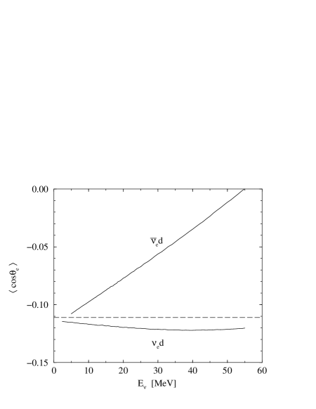
FIG. 3.: The average lepton cosine for the charged-current deuteron reactions, versus the neutrino or antineutrino energy, using Kubodera’s calculations. We plot only from 1 MeV above threshold, so the $v_{e}$-dependence at low energies is not shown. The small jitters are due to the coarse integration grid.

III Applications of the positron angular distribution

A SN1987A events

Supernova 1987A was observed in two water-Čerenkov detectors, Kamiokande II [14] and IMB [15], with 12 and 8 events, respectively. These events were presumably entirely due to $\bar{\nu}_{e}+p\rightarrow e^{+}+n$, with an angular distribution of the form $1+a\cos\theta$. A well-known peculiarity of the SN1987A data is that the angular distributions of the detected positrons are apparently too forward, with $\langle\cos\theta\rangle=0.34$ in Kamiokande II and $\langle\cos\theta\rangle=0.48$ in IMB. Using the results of Fig. 2, evaluated at the observed average energies, and the correction for the IMB angular bias [15], we would expect only $\langle\cos\theta\rangle\simeq 0$ in Kamiokande II and $\langle\cos\theta\rangle\simeq 0.08$ in IMB.

The error on the mean $\langle\cos\theta\rangle$ is

$$\delta\left(\langle\cos\theta\rangle\right)=\frac{1}{\sqrt{N}}\sqrt{\frac{1}{3}-\frac{a^{2}}{3^{2}}}\simeq\frac{1}{\sqrt{3N}}\,,$$ (38)

since $|a|\ll 1$. Thus the expected error on $\langle\cos\theta\rangle$ from just statistics is 0.17 for Kamiokande II and 0.20 for IMB. The range of antineutrino energies contributing only negligibly increases the error. Thus the experimental results for both Kamiokande II and IMB deviate by $+2$-$\sigma$ from the expectations. (The disagreement between the experimental results and the expectations is also discussed in Refs. [10, 16]). At the same time, however, after correcting for the energy difference and the IMB angular bias, the two means are in good agreement with each other.

It is generally assumed in the literature that the angular distributions of Kamiokande II and IMB are consistent. For example, Ref. [17] claims an 81% Kolmogorov-Smirnov probability that the distributions are the same. That test is primarily sensitive to differences in means [18], and so this confirms the agreement of the $\langle\cos\theta\rangle$ values above. However, the angular distribution is also characterized by its variance $\langle\cos^{2}\theta\rangle-\langle\cos\theta\rangle^{2}$, with the expectation being $\simeq 1/3$. The error on the variance is [19]:

$$\delta\left(\langle\cos^{2}\theta\rangle-\langle\cos\theta\rangle^{2}\right)\simeq\frac{1}{\sqrt{N}}\sqrt{\frac{1}{5}-\frac{1}{3^{2}}}\simeq\frac{0.30}{\sqrt{N}}\,.$$ (39)

The experimental result for the variance in Kamiokande II is 0.32, with expected error 0.09, and hence in excellent agreement with expectation. The experimental result for IMB is 0.11, with expected error 0.11, and hence a $-2$-$\sigma$ deviation from expectation and, more importantly, from the Kamiokande II result. Thus, contrary to general belief, the Kamiokande II and IMB angular distributions, characterized here by their first two moments, are not consistent at the 2-$\sigma$ level.

It is possible that some of the observed forward events were due to neutrino-electron scattering, though the expectation is only $\simeq 0.3$ events for Kamiokande II and $\simeq 0.1$ events in IMB (using the same supernova parameters as in Ref. [20] and the detector properties taken from Refs. [14, 15]). Most other authors have also obtained an expectation of $\lesssim 1$ event per detector. Allowing $n$ neutrino-electron scattering events out of a total of $N$ events will change the expectations for the mean $\langle\cos\theta\rangle$ (increased by $n/N$) and the variance $\langle\cos^{2}\theta\rangle-\langle\cos\theta\rangle^{2}$ (increased by $2/3(n/N)-(n/N)^{2}$). Thus for $N\simeq 10$ and the possible $n=1$, the means would be somewhat improved (now each a $+1.5$-$\sigma$ deviation). The Kamiokande II variance would still be in agreement with expectation, though the IMB variance would then be a $-3$-$\sigma$ deviation.

As a general caution about the small-number statistics, one can consider, for the purpose of illustration, the effect of assuming that one backward event was missed. That is, to each data set we add one fake backward event. For Kamiokande II, the effect on both the mean and the variance is modest, but for IMB there is a large effect, making the mean only a $+1$-$\sigma$ deviation and putting the variance in agreement with theory. Thus the statistical significance can be very sensitive to small fluctuations, so that the number of sigmas of deviation and the implicit confidence levels should be taken with caution.

In conclusion, the Kamiokande II data seem to require a 2-$\sigma$ statistical fluctuation in the mean, and the IMB data separate 2-$\sigma$ fluctuations in the mean and the variance. It is difficult to explain the observed angular distributions, even taking into account the corrections of Fig. 2 and (somewhat implausibly) allowing $\simeq 1$ neutrino-electron scattering event in each detector. Given the inconsistency between the Kamiokande II and IMB angular distributions, it is probably not legitimate to combine them, thus weakening the argument for new supernova or particle physics that could have affected the angular distributions, as invoked in Refs. [17, 21, 22]. While we have not explained the angular distributions, we have explicitly shown the perils of the small-number statistics and an apparent additional problem with the IMB results.

B Supernova antineutrinos

A strong $\bar{\nu}_{e}$ signal is expected in SuperKamiokande [23] and other underground detectors from a future Galactic supernova (for the expected count rates see, e.g., Refs. [20, 24]). Is it possible to use the observed angular distribution of the positron events to locate the direction of the supernova [25]? If the $M\rightarrow\infty$ limit were appropriate (i.e., Eq. (24)), then the positrons would be dominantly moving in the backward direction. However, the $1/M$ corrections calculated above are very important. Folding in the expected Fermi-Dirac distribution of the incoming $\bar{\nu}_{e}$, and weighting $\cos\theta$ properly with the flux and cross section calculated here, we arrive at $\langle\cos\theta\rangle\simeq$ 0.015, 0.025 and 0.034 for temperatures $T$ = 4, 5, and 6 MeV. Thus the positrons from supernova $\bar{\nu}_{e}$, with most probable temperature of about 5 MeV, will in fact be slightly forward and, moreover the asymmetry coefficient will sensitively depend on the antineutrino temperature, quite different from the naive expectation. For locating the supernova, the best strategy seems to be to concentrate on the positrons of the highest energy. For $T=5$ MeV, about 25% of the signal will be above 30 MeV, and should have a noticeable forward asymmetry ($\langle\cos\theta\rangle$ = 0.056). Observation of the angular distribution of the higher energy positrons would constitute an important check of the supernova origin of the signal, and would allow location of the supernova to about $\delta(\cos\theta)\simeq 0.2$ [25].

If the supernova direction is known, then knowledge of the positron angular distribution could be used to separate these events from other reactions. For example, if there are $\nu_{\tau}\rightarrow\nu_{e}$ oscillations, then the reaction $\nu_{e}+^{16}{\rm O}\rightarrow e^{-}+^{16}{\rm F}$ can become important [26] (since the $\nu_{\tau}$ temperature is higher than the $\nu_{e}$ temperature and this reaction has a relatively high threshold). The outgoing electrons are somewhat backward. Note that the neutron in $\bar{\nu}_{e}+p\rightarrow e^{+}+n$ is not detected, and electrons and positrons are indistinguishable by their Čerenkov radiation. Therefore, the search for events from $\nu_{e}+^{16}{\rm O}\rightarrow e^{-}+^{16}{\rm F}$ must be done statistically, by looking at the total angular distribution and looking for a backward excess over what is expected from $\bar{\nu}_{e}+p\rightarrow e^{+}+n$ alone. The calculation in Ref. [27] used the naive positron asymmetry $a^{(0)}$ and would have to be revised. Since there would be fewer backward events than they expected, the sensitivity would be improved.

In a heavy water detector like the Sudbury Neutrino Observatory [28], the angular distributions of the outgoing leptons in the reactions $\bar{\nu}_{e}+d\rightarrow e^{+}+n+n$ and $\nu_{e}+d\rightarrow e^{-}+p+p$ could also be used to locate the supernova direction. Because of the low numbers of events, however, even with a naive asymmetry of $a^{(0)}=-1/3$, the pointing resolution is only about $\delta(\cos\theta)\simeq 0.5$ [25]. Taking into account the $1/M$ effects weakens the positron asymmetry, and would degrade the pointing. However, the corrected angular distributions will still be quite important for separating reactions.

C Search for solar antineutrinos

Ref. [29] discusses the possibility of searching in SuperKamiokande for $\bar{\nu}_{e}$ antineutrinos from the Sun, presumably from $\nu_{e}\rightarrow\bar{\nu}_{e}$ oscillations, with $E_{\nu}\sim 10$ MeV. The authors proposed that these events could be separated statistically by their angular distribution from the isotropic detector background and the forward-peaked solar neutrino events from neutrino-electron scattering. However, from Fig. 2, the angular asymmetry is substantially weaker than they assumed, and in view of that, their derived limit would have to be modified.

D LSND results

Another important application of the positron angular distribution is the search for neutrino oscillations by the LSND [1] and KARMEN [2] collaborations. The LSND collaboration reported evidence for $\bar{\nu}_{\mu}\rightarrow\bar{\nu}_{e}$ oscillations following $\mu^{+}$ decay at rest. The evidence is based on the observation of 22 $e^{+}$ + neutron events with positron energies between 36 and 60 MeV, presumably originating from the $\bar{\nu}_{e}p$ interaction. The directions of individual candidate positron events have been measured with respect to the beam axis and the angular distribution is given in Fig. 21 of Ref. [1]. The measured $\langle\cos\theta\rangle$ was found to be $0.20\pm 0.13$.

From our Fig. 2, one would estimate that the expected value would be only about 0.08. However, there are important experimental corrections particular to LSND which must be taken into account. The physics basis of most of them is the simple fact that, for a fixed antineutrino energy $E_{\nu}$, the forward-going positrons have more energy than the backward-going ones. Thus, if there is a cut on positron energy, say $E_{e^{+}}\geq 36$ MeV, then at the lowest allowed antineutrino energies, only the forward positrons will survive the cut, biasing $\langle\cos\theta\rangle$ to be larger. (A similar effect occurs due to the energy-dependent efficiency for positron detection.) These and related effects increase the expected value of $\langle\cos\theta\rangle$ to 0.16, in good agreement with observation [30]. This suggests that LSND is indeed observing $\bar{\nu}_{e}+p\rightarrow e^{+}+n$ events, whatever the origin of the $\bar{\nu}_{e}$.

E Relation to neutron beta decay parameters

It is worth noting that the parameter $a(E_{\nu})$ is the correlation coefficient $a$ between the positron and antineutrino momenta in neutron beta decay  [31]. The parameter $a$ is difficult to measure in neutron beta decay, since the antineutrino momentum can be reconstructed only by measuring the proton recoil momentum. The last measurement [32], more than 20 years ago, yielded $a=-0.102\pm 0.005$. It is tempting to speculate that it might be alternatively measured with $\bar{\nu}_{e}+p\rightarrow e^{+}+n$ via measurement of the positron energy and angle.

It must be pointed out, however, that even at modest $E_{\nu}$, weak magnetism is an important correction, and thus a measurement of $a(E_{\nu})$ would probe a combination of $f$, $g$, and $f_{2}$, thus providing instead a possible test of weak magnetism. To pursue this speculation further, consider an experiment in which $\langle\cos\theta\rangle$ could be measured at a fixed $E_{\nu}$, and consider how well the value of $(f+f_{2})$ could be measured. That is, an experimental test of whether the value of $(f+f_{2})$ extracted matches the value (4.706) predicted by the Conserved Vector Current hypothesis [33]. The expectation for $\langle\cos\theta\rangle$ is approximately given by Eq. (36). From statistics alone, $\delta(\langle\cos\theta\rangle)\simeq 1/\sqrt{3N}$ for $N$ events, so that

$$\delta(f+f_{2})=\frac{\partial(f+f_{2})}{\partial\langle\cos\theta\rangle}\delta(\langle\cos\theta\rangle)\simeq\frac{2}{E_{\nu}/M}\frac{1}{\sqrt{N}}\,.$$ (40)

We assume the standard $V-A$ theory and neglect the (small) form factor variation. Some previous tests of weak magnetism were made by measuring extremely small distortions in the beta spectra of the $A=12$ and $A=20$ systems (see Refs. [34, 35] for a review). These experiments reached a precision on $(f+f_{2})$ of about 10%.

As noted above, for a Galactic supernova at 10 kpc, observed in SuperKamiokande, $\simeq 10^{4}$ $\bar{\nu}_{e}+p\rightarrow e^{+}+n$ events are expected. The time distribution of events is of course irrelevant. The spectrum $f(E_{\nu})$ is also irrelevant insofar as it will be determined from the data, since the measured $E_{e}$ and $\cos\theta_{e}$ can be used to reconstruct $E_{\nu}$ for each event. At each value of $E_{\nu}$, $\langle\cos\theta\rangle$ and hence $(f+f_{2})$ could be measured. While the typical energy expected is $\simeq 20$ MeV, about 2/3 of the events are at higher energies. Thus one might plausibly expect that a test of weak magnetism at the $\simeq 20\%$ level might be made (note also that the error varies linearly with the assumed supernova distance).

IV The neutron angular distribution and applications

It is also of interest to consider the angular distribution of the neutrons from $\bar{\nu}_{e}+p\rightarrow e^{+}+n$, since the neutrons are often detected as well. In fact, the observation of the neutron capture in a delayed coincidence with the positron is the distinguishing signature of the antineutrino interaction with protons, allowing suppression of backgrounds.

There is an angular correlation between the antineutrino direction and the initial direction of the neutron. Since in the laboratory system the proton is at rest, momentum conservation requires that

$$\vec{p}_{\nu}=\vec{p}_{e}+\vec{p}_{n}\,.$$ (41)

Also,

$$|p_{e}|\leq\sqrt{(E_{\nu}-\Delta)^{2}-m_{e}^{2}}<E_{\nu}\,,$$ (42)

so that the neutron must always be emitted in the forward hemisphere. In fact, the maximum angle $(\theta_{n})_{max}$ between the antineutrino and initial neutron directions is achieved when the neutron and and positron momenta are perpendicular. Neglecting ${\cal O}(1/M)$, this is

$$\cos(\theta_{n})_{max}=\frac{\sqrt{2E_{\nu}\Delta-(\Delta^{2}-m_{e}^{2})}}{E_{\nu}}\,.$$ (43)

At threshold, the neutron direction is purely forward, and at reactor energies, still largely so. In Fig. 4 we plot the quantity $\cos(\theta_{n})_{max}$ as well as the average $\langle\cos(\theta_{n})\rangle$, both evaluated numerically, where the latter was weighted with the differential cross section. At ${\cal O}(1/M)$ (see Eq. (15)), the neutron kinetic energy is

$$T_{n}=\frac{E_{\nu}E_{e}^{(0)}}{M}\left(1-v_{e}^{(0)}\cos\theta\right)+\frac{y^{2}}{M}\,.$$ (44)

FIG. 4.: The average neutron cosine and the cosine of the maximum neutron angle versus antineutrino energy. Note that $\cos(\theta_{n})_{max}\rightarrow 1$ both at threshold and as $E_{\nu}\rightarrow\infty$.

It is often possible to localize, at least crudely, the points where positron annihilated (essentially the point of creation for targets with an appreciable density) and where the neutron was captured. Even though the neutron is captured only after many elastic scatterings, its final position maintains some memory of its initial direction, as we now show. For a monoenergetic source of neutrons moving initially along the $x$-axis, the distribution of final positions is Gaussian distributed, with equal widths $\sigma_{x}$, $\sigma_{y}$, and $\sigma_{z}$. The average final position $\langle x\rangle$ is displaced from the origin, and $\langle y\rangle=\langle z\rangle=0$.

We show the results of our Monte Carlo simulation in Fig. 5, implemented by following the principles given by Fermi [36]. We assumed a liquid of $\left({\rm CH_{2}}\right)_{n}$, with or without Gd doping (0.1% by mass), and a density of 0.80 g/cm³. The results in Fig. 5 can easily be rescaled to another density by multiplying by $(0.80/\rho)$. Neutrons are moderated by elastic scattering until they reach thermal energy. At thermal energy, elastic scattering changes the neutron direction, but, on average, not its energy. We also implement capture on protons and Gd. The calculated capture times on undoped and doped scintillator are in good agreement with expectation.

FIG. 5.: The shift (solid line) $\langle x\rangle$ and width (long-dashed line) $\sigma_{x}=\sqrt{\langle x^{2}\rangle-\langle x\rangle^{2}}$ for monoenergetic neutrons (initial kinetic energy $T_{n}$) emitted from the origin, moving initially along the $x$-axis. Note $\langle y\rangle=\langle z\rangle=0$, and $\sigma_{x}=\sigma_{y}=\sigma_{z}$. We used a $\left({\rm CH_{2}}\right)_{n}$ liquid of density 0.80 g/cm³, with or without 0.1% Gd doping by mass.

The most significant input is the fact that the neutron elastic scattering cross sections are almost independent of energy from about 10 keV down to about 0.1 eV [37]. For the first $\sim 5$ scatterings, the neutron maintains some sense of its initial direction, with the angular distribution at a given scattering depending only on the ratio of incoming and outgoing energies. This stage determines $\langle x\rangle\simeq 1.7$ cm, the average displacement of the final point from the starting point. All subsequent scatters only enlarge the size of the neutron cloud. The width $\sigma_{x}$ does depend on the the initial neutron energy because at higher energies more scatterings are required to moderate the neutron to thermal energy.

Above 10 keV, the variation of the cross sections with energy should be taken into account; doing so would increase $\langle x\rangle$ and $\sigma_{x}$ somewhat for $T_{n}\simeq 100$ keV and more substantially for higher energies. Below about 0.1 eV, there is a chemical binding effect depending on the moderating material that increases the cross section; taking that into account would make $\sigma_{x}$ smaller. Finally, from Fig. 4, the struck neutron is not exactly forward, as assumed, but has $\cos\theta_{n}\simeq 0.9$ for reactor energies. Taking that into account would reduce our shift to $\langle x\rangle\simeq 1.5$ cm, in agreement with the results of Ref. [38].

In fact, in the Gösgen reactor antineutrino experiment [39] the neutron displacement was clearly observed, at $\simeq 10\sigma$ level [40]. This was possible because the detector was composed of alternating walls of scintillator and ${}^{3}{\rm He}$ neutron detectors. For a given wall of scintillator in which the reaction occurred, and the positron was detected, more neutrons were observed in the ${}^{3}{\rm He}$ slab away from the reactor than towards the reactor (in fact, the ratio was about 2:1). A similar effect was observed [41] in the Bugey 3 experiment [42], also using a segmented detector.

The neutron-positron separation is also being used [38] by the Chooz experiment [43], which is based on an unsegmented detector. The neutron position is only detected with a precision of about 20 cm, but nevertheless a statistically significant displacement of positron and neutron detection positions along the antineutrino direction is seen.

Given a reliable calculation of the neutron transport in the detector, and hence the expected neutron distributions, this technique would allow a direct determination of the detector background from the measured asymmetry. Such an analysis is being pursued for the Palo Verde reactor experiment, and a forward-backward asymmetry between different cells is seen in the current data [44].

V Conclusions

We have given an expression for the differential cross section in the positron $\cos\theta$, valid to order $1/M$. Recoil and weak magnetism corrections have a large energy-dependent effect on the positron angular distribution, changing it from slightly backward at low energies to isotropic at about 15 MeV and slightly forward at higher energies.

Our main result for the total cross section, valid to order $1/M$, is obtained by integrating Eq. (18). At low energies, this agrees with the well-known $M\rightarrow\infty$ result. At high energies, where the threshold can be neglected, this is in good agreement with Eq. (3.18) of Ref. [6], which contains all orders in $1/M$ but assumes $\Delta=0$. Using our result, we have determined the largest $\Delta$-dependent terms missing in the results of Ref. [6]. The most accurate formula for the total cross section at all energies is obtained by using the result of Ref. [6] with our modifications. The modified formula is essentially identical to our main result for $E_{\nu}\lesssim 30$ MeV and is in good agreement with it (and the unmodified result of Ref. [6]) at higher energies.

The positron angular distribution is well-described by $\langle\cos\theta\rangle$. Our main result, Eq. (34), valid to order $1/M$, is an excellent approximation over the entire energy range considered (and in fact up to about $E_{\nu}\simeq 150$ MeV).

A number of experimental applications are discussed in which the correct angular distribution is necessary for separating $\bar{\nu}_{e}+p\rightarrow e^{+}+n$ events from other reactions and from detector backgrounds.

The neutron angular distribution is initially strongly forward. The random walk of the neutrons as they are moderated acts to erase this. However, the centroid of the final distribution of neutron capture positions is shifted in the direction of the initial motion. We discuss how this can be exploited experimentally.

A Kinematic relations

In the center of momentum frame, the threshold is defined by the positron and neutron being produced at rest, so

$$E_{\nu}^{thr.}=\frac{(M_{n}+m_{e})^{2}-M_{p}^{2}}{2(M_{n}+m_{e})}=1.803{\rm\ MeV}\,.$$ (A1)

In the laboratory frame (where the proton is at rest), the threshold is

$$E_{\nu}^{thr.}=\frac{(M_{n}+m_{e})^{2}-M_{p}^{2}}{2M_{p}}=1.806{\rm\ MeV}\,.$$ (A2)

Labeling the 4-momenta as $\bar{\nu}_{e}(p_{\nu})+p(p_{p})\rightarrow e^{+}(p_{e})+n(p_{n})$, we define the Mandelstam variables as

$$s = (p_{\nu}+p_{p})^{2}=M_{p}^{2}+2M_{p}E_{\nu}$$ (A3)

$$t = (p_{\nu}-p_{e})^{2}=M_{n}^{2}-M_{p}^{2}-2M_{p}(E_{\nu}-E_{e})$$ (A4)

$$u = (p_{\nu}-p_{n})^{2}=M_{p}^{2}+m_{e}^{2}-2M_{p}E_{e}\,,$$ (A5)

evaluated in the laboratory frame, where we can also write $t=q^{2}=m_{e}^{2}-2E_{\nu}E_{e}(1-v_{e}\cos\theta)$.

The differential cross section in $t$ can be written as

$$\frac{d\sigma}{dt}=\frac{G_{F}^{2}\cos^{2}\theta_{C}}{\pi}\frac{|{\cal M}|^{2}}{(s-M_{p}^{2})^{2}}\;(1+\Delta^{R}_{inner})\,,$$ (A6)

where $|{\cal M}|^{2}$ is the amplitude squared (averaged over initial spins, summed over final spins). This can be written as the differential cross section in the positron $\cos\theta$ in the laboratory by using the Jacobian

$$\frac{dt}{d\cos\theta}=2E_{\nu}p_{e}^{(1)}\left[1-\frac{E_{\nu}}{M}\left(1-\frac{1}{v_{e}^{(0)}}\cos\theta\right)+{\cal O}\left(\frac{1}{M^{2}}\right)\right]\,.$$ (A7)

The differential cross section in $E_{e}$ can be obtained by using $dq^{2}/dE_{e}=2M_{p}$.

REFERENCES

- [1] C. Athanassopoulos et al., Phys. Rev. C 54, 2685 (1996); C. Athanassopoulos et al., Phys. Rev. Lett. 77, 3082 (1996).
- [2] B. Armbruster et al., Phys. Rev. C 57, 3414 (1998); K. Eitel et al., hep-ex/9809007.
- [3] P. Vogel, Phys. Rev. D 29, 1918 (1984).
- [4] S. A. Fayans, Sov. J. Nucl. Phys. 42, 590 (1985).
- [5] D. Seckel, hep-ph/9305311.
- [6] C. H. Llewellyn Smith, Phys. Rep. 3, 261 (1972).
- [7] D.H. Wilkinson, Z. Phys. A 348, 129 (1994); A. Sirlin, in Precision Tests of the Standard Model, edited by P. Langacker (World Scientific, Singapore, 1995); J.C. Hardy and I.S. Towner, nucl-th/9812036.
- [8] D.H. Wilkinson, Nucl. Phys. A377, 474 (1982); D.H. Wilkinson, Nucl. Instrum. Methods A 404, 305 (1998).
- [9] Y. Declais et al., Phys. Lett. B 338, 383 (1994).
- [10] D. H. Perkins, in Ninth Workshop on Grand Unification, edited by R. Barloutard (World Scientific, Singapore, 1988).
- [11] K. Kubodera, private communication.
- [12] K. Kubodera, S. Nozawa, Int. J. Mod. Phys. E 3, 101 (1994).
- [13] A.B. Dobrotsvetov and S.A. Fayans, Phys. At. Nucl. 56, 455 (1993).
- [14] K. Hirata et al., Phys. Rev. Lett. 58, 1490 (1987); K.S. Hirata et al., Phys. Rev. D 38, 448 (1988).
- [15] R.M. Bionta et al., Phys. Rev. Lett. 58, 1494 (1987); C.B. Bratton et al., Phys. Rev. D 37, 3361 (1988).
- [16] M.I. Krivoruchenko, Z. Phys. C 44, 633 (1989); T. Konishi et al., Phys. Rev. D 47, 5228 (1993).
- [17] J.M. LoSecco, Phys. Rev. D 39, 1013 (1989).
- [18] W.H. Press et al., Numerical Recipes in FORTRAN, 2nd ed. (Cambridge University Press, 1992).
- [19] A. Stuart and J.K. Ord, Kendall’s Advanced Theory of Statistics, Vol. 1, 6th ed. (John Wiley, New York, 1994).
- [20] J.F. Beacom and P. Vogel, Phys. Rev. D 58 (1998) 053010.
- [21] J.C. van der Velde, Phys. Rev. D 39, 1492 (1989).
- [22] D. Kielczewska, Phys. Rev. D 41, 2967 (1990).
- [23] M. Nakahata et al., Nucl. Instrum. Meth. A421, 113 (1998); Y. Fukuda et al., Phys. Rev. Lett. 81, 1562 (1998); M. Shiozawa et al., Phys. Rev. Lett. 81, 3319 (1998); Y. Fukuda et al., Phys. Rev. Lett. 81, 1158 (1998).
- [24] J.F. Beacom and P. Vogel, Phys. Rev. D 58 (1998) 093012.
- [25] J.F. Beacom and P. Vogel, astro-ph/9811350.
- [26] W.C. Haxton, Phys. Rev. D 36, 2283 (1987).
- [27] Y.-Z. Qian, G.M. Fuller, Phys. Rev. D 49, 1762 (1994).
- [28] H.H. Chen, Phys. Rev. Lett. 55, 1534 (1985); G.T. Ewan et al., Sudbury Neutrino Observatory Proposal, SNO-87-12 (1987); G. Aardsma, et al., Phys. Lett. B 194, 321 (1987); H.H. Chen, Nucl. Instrum. Methods A 264, 48 (1988); G.T. Ewan, Hyperfine Interactions, 103, 199 (1996); M.E. Moorhead, in Neutrino Astrophysics, eds. M. Altmann et al. (Ringberg, Germany, 1997).
- [29] G. Fiorentini, M. Moretti, and F. L. Villante, Phys. Lett. B 413, 378 (1997).
- [30] W.C. Louis, private communication.
- [31] J. D. Jackson, S. B. Treiman, and H. W. Wyld, Phys. Rev. 106, 517 (1957).
- [32] Chr. Stratowa, R. Dobrozemsky, and P. Weinzierl, Phys. Rev. D 18, 3970 (1978).
- [33] M. Gell-Mann, Phys. Rev. 111, 362 (1958).
- [34] V.L. Telegdi, Comments Nucl. Part. Phys. 8, 171 (1979).
- [35] B. Holstein, Weak Interactions in Nuclei (Princeton University Press, Princeton, 1989).
- [36] E. Fermi et al., Nuclear Physics, 2nd ed. (University of Chicago, Chicago, Ill., 1950); see also E. Segrè, Nuclei and Particles, 2nd ed. (Benjamin-Cummings, Reading, Mass., 1977).
- [37] D.J. Hughes and J.A. Harvey, Neutron Cross Sections (Brookhaven National Laboratory, Upton, N.Y., 1955); V. McLane, C.L. Dunford, and P.F. Rose, Neutron Cross Sections, Vol. 2, (Academic Press, New York, 1988).
- [38] C. Bemporad, Neutrino ’98 Conference (June 1998).
- [39] G. Zacek et al., Phys. Rev. D 34, 2621 (1986).
- [40] G. Zacek, Dr. thesis, Technical University of Munich, 1984.
- [41] J.-P. Cussonneau, Dr. thesis, Université de Paris XI (Orsay), 1992.
- [42] Y. Declais et al., Nucl. Phys. B434, 503 (1995).
- [43] M. Apollonio et al., Phys. Lett. B 420 397 (1998).
- [44] F. Boehm, private communication.