Bicocca-FT-99-07

DTP/99/36

hep-ph/9903541

A Phenomenological Study of
Heavy-Quark Fragmentation Functions in $e^{+}e^{-}$ Annihilation

Paolo NASON

INFN, sez. di Milano, Milan, Italy

Carlo OLEARI

Department of Physics, University of Durham, Durham, DH1 3LE, UK

We consider the computation of $D$ and $B$ fragmentation functions in ${e^{+}e^{-}}$ annihilation. We compare the results of fitting present data using the next-to-leading-logarithmic resummed approach, versus the ${\cal O}(\alpha_{s}^{2})$ fixed-order calculation, including also mass-suppressed effects. We also propose a method for merging the fixed-order calculation with the resummed approach.

March 31, 1999

1 Introduction

A theoretical framework for the study of heavy-quark fragmentation functions (HQFF) has been available for a long time [1], and several phenomenological analysis based upon this formalism have appeared in the literature [2, 3, 4]. In Ref. [2], next-to-leading fits to the charm-momentum spectrum at ARGUS were performed and used to predict the bottom spectrum from $Z$ decays. From this analysis, the non-perturbative part of the fragmentation function predicted for the bottom quark turned out to be quite hard: in fact, much harder than predicted in Monte Carlo models using the standard Peterson [5] parametrization. More precise data [6, 7, 8] have become available since then, giving an indication of a hard bottom fragmentation function. In Ref. [3], a study of the charm fragmentation function was performed, using a parametrization of the non-perturbative effects based upon the Peterson fragmentation function, instead of the form adopted in Ref. [2]. A quantitative result on the value of the $\epsilon$ parameter was obtained there, definitely showing that $\epsilon$ is much smaller in next-to-leading-log (NLL) fits rather than in the leading-log (LL) ones.

The interest in further refining our understanding of the fragmentation functions for heavy quark stems mainly from the possibility of using them to improve our understanding of heavy-flavour hadroproduction and photoproduction. In Ref. [9], a formalism for the computation of heavy-flavour production, that merges the high-transverse-momentum approach (i.e. the fragmentation-function approach) and the fixed-order one, was developed. It was found there that mass-suppressed effects are quite large even at moderately large transverse momenta. This work is a first step towards a sound application of the fragmentation-function formalism in the moderate-transverse-momentum range. It should, however, be complemented by similar calculations in the context of ${e^{+}e^{-}}$ annihilation, since this is the place where the impact of non-perturbative effects is studied. This is in fact the purpose of the present work: to use all the available knowledge on heavy-flavour production in ${e^{+}e^{-}}$ annihilation in order to reach an assessment of the size of non-perturbative effects.

There are theoretical approaches to the fragmentation-function calculation that rely upon heavy-quark effective theory in order to study more systematically non-perturbative effects [10]. In the present work, however, we want to establish a connection with the most commonly used parametrization, and thus we will use the Peterson form throughout.

Fixed-order (FO) calculations of the ${\cal O}\left(\alpha_{s}^{2}\right)$ differential cross section for heavy-quark production in $e^{+}e^{-}$ annihilation [11, 12, 13] do exist today, and some applications in the context of HQFF [14, 15] have already appeared. In practice, the fixed-order calculation should be more reliable than the HQFF approach for small annihilation energies. It is interesting, therefore, to consider an approach in which the fixed-order and the HQFF calculations are merged, in the spirit of the work of Ref. [9], without overcounting. In the following, we will thus review the HQFF and the fixed-order-calculation results on fragmentation functions. We will then define a merged approach, in which the fixed-order result is supplemented with leading and next-to-leading logarithmically-enhanced contributions at all orders in $\alpha_{s}$. We will consider both charm- and bottom-production data, which we fit using a Peterson parametrization of the non-perturbative contribution.

The paper is organized as follows. In Section 2 we fix our notation, and describe the aim of our improved approach. In Section 3 we describe the procedure we use in order to incorporate a parametrization of the non-perturbative effects in our formalism. This procedure is to some extent arbitrary. It is however important that the same procedure is used throughout our calculation. In Section 4 we describe the fixed-order calculation of the fragmentation function. Some subtleties, related to its normalization, are discussed in detail. Section 5 is dedicated to the computation of the resummed cross section truncated to order $\alpha_{s}^{2}$, at the NLL level (TNLL). This calculation is almost equivalent to neglecting all mass-suppressed terms (i.e. terms that vanish like powers of $m^{2}/E^{2}$) in the FO calculation, except that terms of order $\alpha_{s}^{2}$, without any power of $\log{E^{2}/m^{2}}$, are not included here. In this section we spell out the definition of the improved approach, and clarify its practical implementation. In Section 6 we compare the various approaches, and in Section 7 we describe our fits to various data sets. Finally, in Section 8, we give our conclusions.

2 Theoretical framework

We consider the inclusive production of a heavy quark $Q$ of mass $m$

$$e^{+}e^{-}\,\mbox{$\rightarrow$}\,Z/\gamma\;(q)\,\mbox{$\rightarrow$}\,Q\,(p)+X\;,$$ (2.1)

where $q$ and $p$ are the four-momenta of the intermediate boson and of the final quark. Defining $x_{E}$ as the scaled energy of the final heavy quark

$$x_{E}={2\,p\cdot q\over q^{2}}\;,$$ (2.2)

and introducing the centre-of-mass energy $E=\sqrt{q^{2}}$, we have the physical constraint

$$\sqrt{\rho}\leq x_{E}\leq 1\;,$$ (2.3)

where

$$\rho={4\,m^{2}\over E^{2}}\;.$$ (2.4)

At times, we will instead use the normalized momentum fraction, defined as

$$x_{p}={\sqrt{x_{E}^{2}-\rho}\over\sqrt{1-\rho}}\;,\quad\quad 0\leq x_{p}\leq 1\>.$$ (2.5)

The inclusive cross section for the production of a heavy quark can be written as a perturbative expansion in $\alpha_{s}$

$${d\sigma\over dx_{p}}(x_{p},E,m)=\sum_{n=0}^{\infty}a^{(n)}(x_{p},E,m,\mu)\,{}\bar{\alpha}_{s}^{n}(\mu)\;,$$ (2.6)

where $\mu$ is the renormalization scale, and

$${}\bar{\alpha}_{s}(\mu)={\alpha_{s}(\mu)\over 2\pi}\;.$$ (2.7)

If $\mu\approx E\approx m$, the truncation of Eq. (2.6) at some fixed order in the coupling constant can be used to approximate the cross section. An ${\cal O}\left(\alpha_{s}^{2}\right)$ fixed-order calculation for the process (2.1) is available [11, 12, 13], so that we can compute the coefficients of Eq. (2.6) at the ${\cal O}\left(\alpha_{s}^{2}\right)$ level. We thus define the fixed-order result as

$$\left.{d\sigma\over dx_{p}}(x_{p},E,m)\right|_{\rm FO}\!\!\!\!=a^{(0)}(x_{p},E,m)+a^{(1)}(x_{p},E,m)\,{}\bar{\alpha}_{s}(E)+a^{(2)}(x_{p},E,m)\,{}\bar{\alpha}_{s}^{2}(E)\;,$$ (2.8)

where we have taken $\mu=E$ for ease of notation.

If $E\gg m$, large logarithms of the form $\log\left(E^{2}/m^{2}\right)$ appear in the differential cross section (2.6) to all orders in the perturbative expansion. In this limit, if we disregard all power-suppressed terms of the form $m^{2}/E^{2}$, the inclusive cross section can be organized in the expansion

$$\left.{d\sigma\over dx}(x,E,m)\right|_{\rm res}\!\!\!\!\! = \!\sum_{n=0}^{\infty}\beta^{(n)}(x)\,\left({}\bar{\alpha}_{s}(E)\log{E^{2}\over m^{2}}\right)^{n}\!+{}\bar{\alpha}_{s}(E)\sum_{n=0}^{\infty}\gamma^{(n)}(x)\,\left({}\bar{\alpha}_{s}(E)\log{E^{2}\over m^{2}}\right)^{n}$$ (2.9)

$${}+{}\bar{\alpha}_{s}^{2}(E)\sum_{n=0}^{\infty}\delta^{(n)}(x)\,\left({}\bar{\alpha}_{s}(E)\log{E^{2}\over m^{2}}\right)^{n}+\ldots+{\cal O}\left({m^{2}\over E^{2}}\right)\;,$$

where $x$ stands now for either $x_{E}$ or $x_{p}$, since the two variables differ by power-suppressed effects.

We define the leading-logarithmic (LL) approximation as

$$\left.{d\sigma\over dx}(x,E,m)\right|_{\rm LL}\!\!=\sum_{n=0}^{\infty}\beta^{(n)}(x)\,\left({}\bar{\alpha}_{s}(E)\log{E^{2}\over m^{2}}\right)^{n}\;,$$ (2.10)

and the next-to-leading-logarithmic (NLL) one as

$$\left.{d\sigma\over dx}(x,E,m)\right|_{\rm NLL}\!\!\!\!\!=\sum_{n=0}^{\infty}\beta^{(n)}(x)\,\left({}\bar{\alpha}_{s}(E)\log{E^{2}\over m^{2}}\right)^{n}\!\!+{}\bar{\alpha}_{s}(E)\sum_{n=0}^{\infty}\gamma^{(n)}(x)\,\left({}\bar{\alpha}_{s}(E)\log{E^{2}\over m^{2}}\right)^{n}\,.$$ (2.11)

The $\delta^{(n)}$ coefficients define the NNLL terms, that are, as of now, not known.

The expansion of Eq. (2.11) up to order $\alpha_{s}^{2}$ is given by

$$\left.{d\sigma\over dx}(x,E,m)\right|_{\rm NLL}\!\!\!\!\! = \!\beta^{(0)}(x)+{}\bar{\alpha}_{s}(E)\left(\gamma^{(0)}(x)+\beta^{(1)}(x)\log{E^{2}\over m^{2}}\right)$$ (2.12)

$$\!\mbox{}+{}\bar{\alpha}_{s}^{2}(E)\left(\gamma^{(1)}(x)\log{E^{2}\over m^{2}}+\beta^{(2)}(x)\log^{2}{E^{2}\over m^{2}}\right)+{\cal O}\left(\alpha_{s}^{3}\right)\;,\phantom{aaaa}$$

and does not coincide with the massless limit of the FO calculation. A term of order $\alpha_{s}^{2}$, not accompanied by logarithmic factors, may in fact survive in the massless limit of the FO result. In the HQFF approach, this is a NNLL effect, and therefore it is not included at the NLL level. We will refer to this term, in the following, as the NNLL $\alpha_{s}^{2}$ term.

It is now clear how to obtain an improved formula, which contains all the information present in the FO approach, as well as in the HQFF approach. Using Eqs. (2.8) and (2.11), we write the improved cross section as

$$\left.{d\sigma\over dx_{p}}(x_{p},E,m)\right|_{\rm imp}\!\!\!\! = \sum_{i=0}^{2}a^{(i)}(x_{p},E,m)\,{}\bar{\alpha}_{s}^{i}(E)+\sum_{n=3}^{\infty}\beta^{(n)}(x)\,\left({}\bar{\alpha}_{s}(E)\log{E^{2}\over m^{2}}\right)^{n}$$ (2.13)

$${}+{}\bar{\alpha}_{s}(E)\sum_{n=2}^{\infty}\gamma^{(n)}(x)\,\left({}\bar{\alpha}_{s}(E)\log{E^{2}\over m^{2}}\right)^{n}\;,$$

where the LL and NLL sums now start from $n=3$ and $n=2$ respectively, in order to avoid double counting. Formula (2.13) includes exactly all terms up to the order $\alpha_{s}^{2}$ (including mass effects), and all terms of the form $\Big{(}{}\bar{\alpha}_{s}(E)\log\left(E^{2}/m^{2}\right)\Big{)}^{n}$ and ${}\bar{\alpha}_{s}(E)\,\Big{(}{}\bar{\alpha}_{s}(E)\log\left(E^{2}/m^{2}\right)\Big{)}^{n}$, so that it is also correct at NLL level for $E\gg m$. It can be viewed as an interpolating formula. For moderate energies, it is accurate to the order $\alpha_{s}^{2}$, while for very large energies it is accurate at the NLL level.

3 Non-perturbative effects

In the HQFF formalism, the inclusive heavy-flavour cross section is given by the formula

$${d\sigma\over dx}(x,E,m) = \sum_{i}{d\hat{\sigma}_{i}\over dx}\left(x,E,\mu_{F}\right)\,\otimes\hat{D}_{i}\left(x,\mu_{F},m\right)$$ (3.1)

$$= \sum_{i}\int_{x}^{1}{dz\over z}\,{d\hat{\sigma}_{i}\over dz}\left(z,E,\mu_{F}\right)\,\hat{D}_{i}\left({x\over z},\mu_{F},m\right)\;,$$

where $d\hat{\sigma}_{i}(x,E,\mu_{F})/dx$ are the $\overline{\rm MS}$-subtracted partonic cross sections for producing the parton $i$, and $\hat{D}_{i}(x,\mu_{F},m)$ are the $\overline{\rm MS}$ fragmentation functions for parton $i$ to evolve into the heavy quark $Q$. The factorization scale $\mu_{F}$ must be taken of order $E$ in order to avoid the appearance of large logarithms of $E/\mu_{F}$ in the partonic cross section. The explicit expressions for the partonic cross sections and for the fragmentation functions at NLO can be found in Refs. [1, 16].

The weak point of formula (3.1) comes from the initial condition for the evolution of the fragmentation function, which is computed as a power expansion in terms of $\alpha_{s}(m)$. In particular, irreducible, non-perturbative uncertainties of order $\Lambda_{\scriptscriptstyle\rm QCD}/m$ are present. We assume that all these effects are described by a non-perturbative fragmentation function $D_{\rm NP}^{H}$, that takes into account all low-energy effects, including the process of the heavy quark turning into a heavy-flavoured hadron. The full resummed cross section, including non-perturbative corrections, is then written as

$${d\sigma^{H}\over dx}(x,E,m) = \sum_{i}{d\hat{\sigma}_{i}\over dx}\left(x,E,\mu_{F}\right)\,\otimes\hat{D}_{i}\left(x,\mu_{F},m\right)\otimes D_{\rm NP}^{H}(x)\;.$$ (3.2)

We will parametrize the non-perturbative part of the fragmentation function with the Peterson form

$$D_{\rm NP}^{H}(x)=P(x,\epsilon)\equiv N\,{x\,(1-x)^{2}\over\left[(1-x)^{2}+x\,\epsilon\right]^{2}}\;,$$ (3.3)

where the normalization factor $N$ determines the fraction of the hadron of type $H$ in the final state. Summing over all hadron types, we have the condition

$$\sum_{H}\int_{0}^{1}dx\,D_{\rm NP}^{H}(x)=1\;.$$ (3.4)

4 The $\alpha_{s}^{2}$ fixed-order approach

We define our fixed-order cross section, supplemented with non-perturbative fragmentation effects, by the convolution of the perturbative cross section (2.8) with the non-perturbative fragmentation function (3.3)

$$\left.{d\sigma^{H}\over dx_{p}}(x_{p},E,m)\right|_{\rm FO}\!\!\!\! = \int_{0}^{1}dy\,dz_{p}\left.{d\sigma\over dz_{p}}(z_{p},E,m)\right|_{\rm FO}\!\!\!\!P(y,\epsilon)\,\delta(x_{p}-yz_{p})$$ (4.1)

$$= \int_{0}^{1}dy\,dz_{p}\sum_{i=0}^{2}a^{(i)}(z_{p},E,m)\,{}\bar{\alpha}_{s}^{i}(E)\;P(y,\epsilon)\,\delta(x_{p}-yz_{p})\;.$$

It is assumed, in this formula, that non-perturbative effects degrade the momentum, rather than the energy of the heavy quark. This is to avoid unphysical results when the momentum is smaller than the mass. It should be made clear, however, that for small momenta this formula should be seen merely as a model for non-perturbative effects.

The coefficients of the perturbative expansion $a^{(i)}(z_{p},E,m)$ are in general distributions in $z_{p}$ with singularities at $z_{p}=1$. In order to deal with these singularities, we transform Eq. (4.1) as follows

$$\left.{d\sigma^{H}\over dx_{p}}\right|_{\rm FO}\!\!\!\! = \int_{0}^{1}dy\,dz_{p}\sum_{i=0}^{2}a^{(i)}(z_{p},E,m)\,{}\bar{\alpha}_{s}^{i}(E)\;P(y,\epsilon)\,\left\{\delta(x_{p}-yz_{p})-\delta(x_{p}-y)\right\}$$ (4.2)

$$+ \int_{0}^{1}dy\,dz_{p}\sum_{i=0}^{2}a^{(i)}(z_{p},E,m)\,{}\bar{\alpha}_{s}^{i}(E)\;P(y,\epsilon)\,\delta(x_{p}-y)$$

$$= P(x_{p},\epsilon)\sum_{i=0}^{2}\bar{a}^{(i)}(E,m)\,{}\bar{\alpha}_{s}^{i}(E)$$

$$+ \int_{0}^{1}dy\,dz_{p}\sum_{i=0}^{2}a^{(i)}(z_{p},E,m)\,{}\bar{\alpha}_{s}^{i}(E)\;P(y,\epsilon)\,\left\{\delta(x_{p}-yz_{p})-\delta(x_{p}-y)\right\},\phantom{aaaa}$$

where

$$\bar{a}^{(i)}(E,m)\equiv\int_{0}^{1}dz_{p}\,a^{(i)}(z_{p},E,m)\;.$$ (4.3)

The $a^{(0)}$ term in the last integral of Eq. (4.2), in fact, does not contribute, since it is proportional to $\delta(1-z_{p})$. We thus find

$$\left.{d\sigma^{H}\over dx_{p}}\right|_{\rm FO}\!\!\!\! = \!\!P(x_{p},\epsilon)\,\sigma_{\rm inc}$$ (4.4)

$$+ \!\!\int_{0}^{1}dy\,dz_{p}\sum_{i=1}^{2}a^{(i)}(z_{p},E,m)\,{}\bar{\alpha}_{s}^{i}(E)\;P(y,\epsilon)\,\left\{\delta(x_{p}-yz_{p})-\delta(x_{p}-y)\right\}\,,\phantom{aaa}$$

where

$$\sigma_{\rm inc}=\bar{a}^{(0)}(E,m)+\bar{a}^{(1)}(E,m)\,{}\bar{\alpha}_{s}(E)+\bar{a}^{(2)}(E,m)\,{}\bar{\alpha}_{s}^{2}(E)\;$$ (4.5)

is the inclusive heavy-quark cross section.

It would be natural to normalize the cross section in terms of the total cross section for heavy-flavoured events. However, for practical purposes, the normalization is immaterial, because of the uncertainty in the specific heavy-flavoured hadron fraction, and it must be fitted to the data. It is important, however, that the normalization factor has a finite massless limit, since the same normalization has to be applied to the resummed cross section. In the present case, neither the total heavy-flavour cross section nor the inclusive cross section are finite in the massless limit. This problem arises because of mass singularities in the coefficient $\bar{a}^{(2)}(E,m)$. We then define

$$\bar{a}^{(2)}(E,m)=\bar{a}_{1Q}^{(2)}(E,m)+2\,\bar{a}_{2Q}^{(2)}(E,m)+\bar{a}_{R}^{(2)}(E,m)\;,$$ (4.6)

where:

• the $1Q$-term consists of all graphs in which the primary interaction vertex is always attached to the heavy flavour, and furthermore there is only one heavy-flavour pair in the final state.

• The $2Q$-term consists of all graphs in which the primary interaction vertex is always attached to the heavy flavour, and there is a secondary heavy-quark pair in the final state coming from the gluon-splitting mechanism. There is a factor of 2 in front of this contribution, since, in the inclusive cross section, both the primary heavy quark and the secondary one can be detected.

• The $R$-term (where $R$ stands for “rest”) contains all other contributions. These include terms in which a heavy-flavour pair is produced via gluon splitting in a process initiated by light quarks, plus interference terms in which a heavy quark (antiquark), produced via gluon splitting in an amplitude, interferes with a heavy quark (antiquark), produced directly at the $Z/\gamma$ vertex.

We define a “normalization” total cross section as

$$\sigma_{\rm n}=\bar{a}^{(0)}(E,m)+\bar{a}^{(1)}(E,m)\,{}\bar{\alpha}_{s}(E)+\left[\bar{a}_{1Q}^{(2)}(E,m)+\bar{a}_{2Q}^{(2)}(E,m)\right]\,{}\bar{\alpha}_{s}^{2}(E)\;.$$ (4.7)

This cross section is finite in the massless limit. In fact, the mass singularities, present in the $\bar{a}_{2Q}^{(2)}(E,m)$ term, cancel against the virtual graphs in $\bar{a}_{1Q}^{(2)}(E,m)$ having a gluon self-energy correction consisting of a heavy-flavour loop.

The analytic expressions of $a^{(0)}(z_{p},E,m)$ and $a^{(1)}(z_{p},E,m)$, and of $\bar{a}^{(0)}(E,m)$ and $\bar{a}^{(1)}(E,m)$, are known (see Refs. [16, 17]). The $a^{(2)}(z_{p},E,m)$ term has been computed by the authors and is available as a numerical FORTRAN program.

The advantage of writing Eq. (4.1) in the form of Eq. (4.4) is that the singularities in the two-jet limit are regularized, and the two-body virtual terms (i.e. $Z/\gamma\,\mbox{$\rightarrow$}\,Q+\overline{Q}$), that are proportional to $\delta(1-z_{p})$, give zero contribution. Thus, the two-loop virtual corrections, which were not computed in Ref. [11], do not contribute there. On the other hand, they contribute to $\bar{a}^{(2)}_{1Q}(E,m)$. They do disappear from our formula, however, if we normalize it to the $\sigma_{\rm n}$ cross section, consistently dropping higher order terms. We obtain

$${1\over\sigma_{\rm n}}\left.{d\sigma^{H}\over dx_{p}}(x_{p},E,m)\right|_{\rm FO}\!\!\!\! = P(x_{p},\epsilon)\,n_{R}+{1\over\bar{a}^{(0)}(E,m)}\int_{0}^{1}dy\,dz_{p}\,\Bigg{\{}a^{(1)}(z_{p},E,m)\,{}\bar{\alpha}_{s}$$ (4.8)

$${}+\left[a^{(2)}(z_{p},E,m)-{\bar{a}^{(1)}(E,m)\over\bar{a}^{(0)}(E,m)}\,a^{(1)}(z_{p},E,m)\right]{}\bar{\alpha}_{s}^{2}\Bigg{\}}$$

$${}\times P(y,\epsilon)\,\left\{\delta(x_{p}-yz_{p})-\delta(x_{p}-y)\right\}\;,$$

where

$$n_{R}=1+{\bar{a}_{2Q}^{(2)}(E,m)+\bar{a}_{R}^{(2)}(E,m)\over\bar{a}^{(0)}(E,m)}\,{}\bar{\alpha}_{s}^{2}(E)\;.$$ (4.9)

Although the $\bar{a}_{R}^{(2)}(E,m)$ term contains all sort of interference contributions, it is dominated by terms in which a primary light-quark pair generates a gluon that decays into a heavy-quark pair. This contribution is singular in the massless limit. An analogous singularity is present in the $\bar{a}_{2Q}^{(2)}(E,m)$ term. Thus, the dominant corrections to $n_{R}$ arise from secondary heavy-quark production via gluon splitting.

Performing the integration in $y$ we can write

$${1\over\sigma_{\rm n}}\left.{d\sigma^{H}\over dx_{p}}(x_{p},E,m)\right|_{\rm FO}\!\!\!\! = P(x_{p},\epsilon)\,n_{R}$$ (4.10)

$${}+\sum_{i=1}^{2}\,{}\bar{\alpha}_{s}^{i}(E)\,\Biggl{\{}\int_{x_{p}}^{1}dz_{p}\,b^{(i)}(z_{p},E,m)\left[{P\left(x_{p}/z_{p},\epsilon\right)\over z_{p}}-P(x_{p},\epsilon)\right]$$

$${}-P(x_{p},\epsilon)\int_{0}^{x_{p}}dz_{p}\,b^{(i)}(z_{p},E,m)\Biggr{\}}\;,$$

where we have defined

$$b^{(1)}(z_{p},E,m) = {a^{(1)}(z_{p},E,m)\over\bar{a}^{(0)}(E,m)}$$

$$b^{(2)}(z_{p},E,m) = {1\over\bar{a}^{(0)}(E,m)}\left[a^{(2)}(z_{p},E,m)-{\bar{a}^{(1)}(E,m)\over\bar{a}^{(0)}(E,m)}\,a^{(1)}(z_{p},E,m)\right]\;.\phantom{aaa}$$ (4.11)

For future use, we introduce here the hadronic differential cross section expressed in term of the energy fraction. From Eq. (2.5), we can write

$${1\over\sigma_{\rm n}}\,{d\sigma^{H}\over dx_{E}}={1\over\sigma_{\rm n}}\,{d\sigma^{H}\over dx_{p}}\,{dx_{p}\over dx_{E}}={1\over\sigma_{\rm n}}\,{d\sigma^{H}\over dx_{p}}\,{x_{E}\over x_{p}}\,{1\over 1-\rho}\;.$$ (4.12)

5 NLL higher-order effects

According to Eq. (2.13), we must add to the FO result all terms of order $\alpha_{s}^{3}$ and higher of the full NLL resummed result. The resummed result is obtained numerically by solving the Altarelli-Parisi evolution equations for the fragmentation functions, with the given ${\cal O}(\alpha_{s})$ initial conditions, convoluted with the appropriate short-distance cross sections. We must, however, subtract, from this numerical result, the terms up to second order of its expansion in powers of $\alpha_{s}$. These terms can be obtained with the same procedure used in Ref. [14]. We recall here the principal steps that give us the ${\cal O}\left(\alpha_{s}^{2}\right)$ terms of the resummed cross section.

We introduce the following notation for the Mellin transform of a generic function $f(x)$:

$$f(N)\equiv\int_{0}^{1}dx\,x^{N-1}f(x)\;.$$ (5.1)

We adopt the convention that, when $N$ appears, instead of $x$, as the argument of a function, we are actually referring to the Mellin transform of the function. This notation is somewhat improper, but it should not generate confusion in the following, since we will work only with Mellin transforms.

The Mellin transform of the factorization theorem (3.1) is given by

$$\sigma(N,E,m)=\sum_{i}\hat{\sigma}_{i}(N,E,\mu)\;\hat{D}_{i}(N,\mu,m)\;,$$ (5.2)

where

$$\sigma(N,E,m)=\int_{0}^{1}dx\,x^{N-1}{d\sigma\over dx}(x,E,m)\;,$$ (5.3)

and a similar one for $\hat{\sigma}_{i}(N,E,\mu)$. The Mellin transform of the Altarelli-Parisi evolution equations is

$${d\hat{D}_{i}(N,\mu,m)\over d\log\mu^{2}}=\sum_{j}{}\bar{\alpha}_{s}(\mu)\left[P_{ij}^{(0)}(N)+P_{ij}^{(1)}(N)\,{}\bar{\alpha}_{s}(\mu)+{\cal O}\left(\alpha_{s}^{2}\right)\right]\hat{D}_{j}(N,\mu,m)\;.$$ (5.4)

We need an expression for $\sigma(N,E,m)$ valid at the second order in $\alpha_{s}$. Thus, we solve Eq. (5.4), with initial condition at $\mu=\mu_{0}$, with an ${\cal O}\left(\alpha_{s}^{2}\right)$ accuracy. This is easily done by rewriting Eq. (5.4) as an integral equation

$$\hat{D}_{i}(N,\mu,m)\!\!\! = \!\!\!\hat{D}_{i}(N,\mu_{0},m)$$ (5.5)

$$+ \!\!\!\sum_{j}\int_{\mu_{0}}^{\mu}d\log{\mu^{\prime}}^{2}\;{}\bar{\alpha}_{s}(\mu^{\prime})\left[P_{ij}^{(0)}(N)+P_{ij}^{(1)}(N)\,{}\bar{\alpha}_{s}(\mu^{\prime})\right]\hat{D}_{j}(N,\mu^{\prime},m)\;.\phantom{aaaaa}$$

The terms proportional to $\alpha_{s}^{2}$ can be evaluated at any scale ($\mu$ or $\mu_{0}$), the difference being of order $\alpha_{s}^{3}$. Factors involving a single power of $\alpha_{s}$ can instead be expressed in terms of $\alpha_{s}(\mu_{0})$ using the renormalization group equation

$${}\bar{\alpha}_{s}(\mu^{\prime}) = {}\bar{\alpha}_{s}(\mu_{0})-2\,\pi\,b_{0}\,{}\bar{\alpha}_{s}^{2}(\mu_{0})\,\log{{\mu^{\prime}}^{2}\over\mu_{0}^{2}}+{\cal O}\left(\alpha_{s}^{3}\left(\mu_{0}\right)\right)$$

$$b_{0} = {11\,C_{A}-4\,n_{f}\,T_{F}\over 12\,\pi}\;,$$ (5.6)

with $n_{f}$ the number of flavours, including the heavy one. Equation (5.5) then becomes

$$\hat{D}_{i}(N,\mu,m) = \hat{D}_{i}(N,\mu_{0},m)+\sum_{j}\int_{\mu_{0}}^{\mu}d\log{\mu^{\prime}}^{2}\;{}\bar{\alpha}_{s}(\mu_{0})P_{ij}^{(0)}(N)\,\hat{D}_{j}(N,\mu^{\prime},m)$$ (5.7)

$${}+\sum_{j}{}\bar{\alpha}_{s}^{2}(\mu_{0})\,P_{ij}^{(1)}(N)\,\hat{D}_{j}(N,\mu_{0},m)\,\log{\mu^{2}\over\mu_{0}^{2}}$$

$${}-2\,\pi\,b_{0}\,\sum_{j}{}\bar{\alpha}_{s}^{2}(\mu_{0})\,P_{ij}^{(0)}(N)\,\hat{D}_{j}(N,\mu_{0},m)\,{1\over 2}\log^{2}{\mu^{2}\over\mu_{0}^{2}}\;.$$

Now we need to express $\hat{D}_{j}(N,\mu^{\prime},m)$ on the right-hand side of the above equation as a function of the initial condition, with an accuracy of order $\alpha_{s}$. This is simply done by iterating the above equation once, keeping only the first two terms on the right-hand side. Our final result is then

$$\hat{D}_{i}(N,\mu,m) = \hat{D}_{i}(N,\mu_{0},m)+\sum_{j}{}\bar{\alpha}_{s}(\mu_{0})P_{ij}^{(0)}(N)\,\hat{D}_{j}(N,\mu_{0},m)\,\log{\mu^{2}\over\mu_{0}^{2}}$$ (5.8)

$${}+\sum_{kj}{}\bar{\alpha}_{s}^{2}(\mu_{0})P_{ik}^{(0)}(N)\,P_{kj}^{(0)}(N)\,\hat{D}_{j}(N,\mu_{0},m)\,{1\over 2}\log^{2}{\mu^{2}\over\mu_{0}^{2}}$$

$${}+\sum_{j}{}\bar{\alpha}_{s}^{2}(\mu_{0})P_{ij}^{(1)}(N)\,\hat{D}_{j}(N,\mu_{0},m)\,\log{\mu^{2}\over\mu_{0}^{2}}$$

$${}-\pi\,b_{0}\,\sum_{j}{}\bar{\alpha}_{s}^{2}(\mu_{0})P_{ij}^{(0)}(N)\,\hat{D}_{j}(N,\mu_{0},m)\,\log^{2}{\mu^{2}\over\mu_{0}^{2}}\;.$$

Using the initial conditions (see Ref. [1])

$$\hat{D}_{Q}(N,\mu_{0},m) = 1+{}\bar{\alpha}_{s}(\mu_{0})\,d^{(1)}_{Q}(N,\mu_{0},m)+{\cal O}\left(\alpha_{s}^{2}\left(\mu_{0}\right)\right)$$

$$\hat{D}_{g}(N,\mu_{0},m) = {}\bar{\alpha}_{s}(\mu_{0})\,d^{(1)}_{g}(N,\mu_{0},m)+{\cal O}\left(\alpha_{s}^{2}\left(\mu_{0}\right)\right)\;,$$ (5.9)

(all the other components being of order $\alpha_{s}^{2}$), and using Eq. (5) to express $\alpha_{s}\left(\mu_{0}\right)$ in terms of $\alpha_{s}\left(\mu\right)$, Eq. (5.8) becomes, with the required accuracy,

$$\hat{D}_{i}(N,\mu,m) = \delta_{iQ}+{}\bar{\alpha}_{s}(\mu)\,d^{(1)}_{i}(N,\mu_{0},m)+2\,\pi\,b_{0}\,{}\bar{\alpha}_{s}^{2}(\mu)\,d^{(1)}_{i}(N,\mu_{0},m)\,\log{\mu^{2}\over\mu_{0}^{2}}$$ (5.10)

$${}+{}\bar{\alpha}_{s}(\mu)P_{iQ}^{(0)}(N)\,\log{\mu^{2}\over\mu_{0}^{2}}+\sum_{j}{}\bar{\alpha}_{s}^{2}(\mu)P_{ij}^{(0)}(N)\,d^{(1)}_{j}(N,\mu_{0},m)\,\log{\mu^{2}\over\mu_{0}^{2}}$$

$${}+\sum_{k}{}\bar{\alpha}_{s}^{2}(\mu)P_{ik}^{(0)}(N)\,P_{kQ}^{(0)}(N)\,{1\over 2}\log^{2}{\mu^{2}\over\mu_{0}^{2}}+{}\bar{\alpha}_{s}^{2}(\mu)P_{iQ}^{(1)}(N)\,\log{\mu^{2}\over\mu_{0}^{2}}$$

$${}+\pi\,b_{0}\,{}\bar{\alpha}_{s}^{2}(\mu)P_{iQ}^{(0)}(N)\,\log^{2}{\mu^{2}\over\mu_{0}^{2}}\;.$$

Using the notation of Ref. [16], we have, for the partonic cross sections,

$$\hat{\sigma}_{Q} = \hat{\sigma}_{\overline{Q}}=\sigma_{0,Q}\left[1+{}\bar{\alpha}_{s}C_{F}c_{Q}+{\cal O}\left(\alpha_{s}^{2}\right)\right]$$

$$\hat{\sigma}_{q} = \hat{\sigma}_{\bar{q}}=\sigma_{0,q}\left[1+{\cal O}\left(\alpha_{s}\right)\right]$$

$$\hat{\sigma}_{g} = \sigma_{0}\left[{}\bar{\alpha}_{s}C_{F}c_{g}+{\cal O}\left(\alpha_{s}^{2}\right)\right]\;,$$ (5.11)

where $Q$ is the heavy quark and $q$ is a light one, and

$$\sigma_{0,Q} = \sigma_{0,Q}^{(v)}+\sigma_{0,Q}^{(a)}$$

$$\sigma_{0,q} = \sigma_{0,q}^{(v)}+\sigma_{0,q}^{(a)}$$

$$\sigma_{0} = \sum_{f=1}^{n_{f}}\sigma_{0,f}=\sigma_{0,Q}+\sum_{q}\sigma_{0,q}$$

$$c_{Q} = c_{T,Q}+c_{L,Q}$$

$$c_{g} = c_{T,g}+c_{L,g}\;,$$ (5.12)

where $v$, $a$, $T$ and $L$ refer to the vector, axial, transverse and longitudinal contributions, respectively.

In addition, we define the Mellin moments

$$\hat{a}_{Q/g}^{(1)}(N,E,\mu)=C_{F}c_{Q/g}(N,E,\mu)\;,$$ (5.13)

and introduce the total “normalization” ${\cal O}\left(\alpha_{s}\right)$ cross section for the production of a heavy quark

$$\sigma_{\rm n}=\sigma_{0,Q}\left[1+{3\over 2}C_{F}{}\bar{\alpha}_{s}+{\cal O}\left(\alpha_{s}^{2}\right)\right]\;.$$ (5.14)

Observe that now, at NLL accuracy, we can neglect the ${\cal O}\left(\alpha_{s}^{2}\right)$ terms, since they do not contain any logarithmic enhancement. This would not be the case for the total heavy-quark cross section, that in fact is divergent at order ${\cal O}\left(\alpha_{s}^{2}\right)$, in the massless limit approximation.

From Eq. (5.2), we can write the NLL cross section as

$$\sigma(N)=\hat{\sigma}_{Q}\,\hat{D}_{Q}+\hat{\sigma}_{\overline{Q}}\,\hat{D}_{\overline{Q}}+\sum_{q}\hat{\sigma}_{q}\,\hat{D}_{q}+\sum_{\bar{q}}\hat{\sigma}_{\bar{q}}\,\hat{D}_{\bar{q}}+\hat{D}_{g}\,\hat{\sigma}_{g}\;,$$ (5.15)

where we have dropped the energy and the mass dependence, for ease of notation.

We can now obtain the truncated ${\cal O}\left(\alpha_{s}^{2}\right)$ NLL (TNLL from now on) normalized cross section as

$$\left.{1\over\sigma_{\rm n}}\sigma(N)\right|_{\rm TNLL}\!\!\!\!\!\!\!\! = \!\!\!\Biggl{\{}1+{}\bar{\alpha}_{s}(\mu)\,d^{(1)}_{Q}(N)+{}\bar{\alpha}_{s}(\mu)P_{QQ}^{(0)}(N)\,\log{\mu^{2}\over\mu_{0}^{2}}+{}\bar{\alpha}_{s}(\mu)\left(\hat{a}_{Q}^{(1)}(N)-{3\over 2}C_{F}\right)$$ (5.16)

$${}\!\!\!+{}\bar{\alpha}_{s}^{2}(\mu)P_{QQ}^{(0)}(N)\left(\hat{a}_{Q}^{(1)}(N)-{3\over 2}C_{F}\right)\log{\mu^{2}\over\mu_{0}^{2}}+2\,\pi\,b_{0}\,{}\bar{\alpha}_{s}^{2}(\mu)\,d^{(1)}_{Q}(N)\,\log{\mu^{2}\over\mu_{0}^{2}}$$

$${}\!\!\!+\sum_{j}{}\bar{\alpha}_{s}^{2}(\mu)P_{Qj}^{(0)}(N)\,d^{(1)}_{j}(N)\,\log{\mu^{2}\over\mu_{0}^{2}}$$

$${}+\sum_{k}{}\bar{\alpha}_{s}^{2}(\mu)P_{Qk}^{(0)}(N)\,P_{kQ}^{(0)}(N)\,{1\over 2}\log^{2}{\mu^{2}\over\mu_{0}^{2}}+{}\bar{\alpha}_{s}^{2}(\mu)P_{QQ}^{(1)}(N)\,\log{\mu^{2}\over\mu_{0}^{2}}$$

$${}\!\!\!+\pi\,b_{0}\,{}\bar{\alpha}_{s}^{2}(\mu)P_{QQ}^{(0)}(N)\,\log^{2}{\mu^{2}\over\mu_{0}^{2}}$$

$${}\!\!\!+{}\bar{\alpha}_{s}^{2}(\mu)P_{\overline{Q}g}^{(0)}(N)\,d^{(1)}_{g}(N)\,\log{\mu^{2}\over\mu_{0}^{2}}+{}\bar{\alpha}_{s}^{2}(\mu)P_{\overline{Q}g}^{(0)}(N)\,P_{gQ}^{(0)}(N)\,{1\over 2}\log^{2}{\mu^{2}\over\mu_{0}^{2}}$$

$${}\!\!\!+{}\bar{\alpha}_{s}^{2}(\mu)P_{\overline{Q}Q}^{(1)}(N)\,\log{\mu^{2}\over\mu_{0}^{2}}\Biggr{\}}$$

$${}\!\!\!+{1\over\hat{\sigma}_{0,Q}}\sum_{q}\hat{\sigma}_{0,q}{}\bar{\alpha}_{s}^{2}(\mu)\Biggl{\{}P_{qg}^{(0)}(N)\,d^{(1)}_{g}(N)\,\log{\mu^{2}\over\mu_{0}^{2}}$$

$${}\!\!\!+P_{qg}^{(0)}(N)\,P_{gQ}^{(0)}(N)\,{1\over 2}\log^{2}{\mu^{2}\over\mu_{0}^{2}}+P_{qQ}^{(1)}(N)\,\log{\mu^{2}\over\mu_{0}^{2}}$$

$${}\!\!\!+P_{\bar{q}g}^{(0)}(N)\,d^{(1)}_{g}(N)\,\log{\mu^{2}\over\mu_{0}^{2}}$$

$${}\!\!\!+P_{\bar{q}g}^{(0)}(N)\,P_{gQ}^{(0)}(N)\,{1\over 2}\log^{2}{\mu^{2}\over\mu_{0}^{2}}+P_{\bar{q}Q}^{(1)}(N)\,\log{\mu^{2}\over\mu_{0}^{2}}\Biggr{\}}$$

$${}\!\!\!+{1\over\hat{\sigma}_{0,Q}}\hat{\sigma}_{0}\hat{a}_{g}^{(1)}(N){}\bar{\alpha}_{s}^{2}(\mu)P_{gQ}^{(0)}(N)\,\log{\mu^{2}\over\mu_{0}^{2}}\;,$$

where we have taken $\mu=E$ and $\mu_{0}=m$, and we have introduced the notation

$$\hat{a}^{(1)}_{Q/g}(N)=\hat{a}^{(1)}_{Q/g}(N,E,\mu)|_{\mu=E}\;,\quad\quad\quad d^{(1)}_{Q/g}(N)=d^{(1)}_{Q/g}(N,\mu_{0},m)|_{\mu_{0}=m}\;.$$ (5.17)

The lowest order splitting functions are given by

$$P^{(0)}_{QQ}(N) = C_{F}\left[{3\over 2}+{1\over N(N+1)}-2\,S_{1}(N)\right]\,,$$

$$P^{(0)}_{Qg}(N) = P^{(0)}_{\overline{Q}g}(N)=P^{(0)}_{qg}(N)=P^{(0)}_{\bar{q}g}(N)=C_{F}\left[{2+N+N^{2}\over N(N^{2}-1)}\right]\,,$$

$$P^{(0)}_{gQ}(N) = T_{F}\left[{2+N+N^{2}\over N(N+1)(N+2)}\right]\,,$$ (5.18)

where

$$S_{1}(N)=\psi_{0}(N+1)-\psi_{0}(1)\,,$$ (5.19)

and

$$\psi_{0}(z)={d\over dz}\log{\Gamma(z)}\;.$$ (5.20)

In addition we have

$$P_{qQ}^{(1)}(N)=P_{\bar{q}Q}^{(1)}(N)=P_{q^{\prime}q}(N)\;,$$ (5.21)

and the splitting functions $P_{QQ}^{(1)}(N)$, $P_{\overline{Q}Q}^{(1)}(N)$ and $P_{q^{\prime}q}(N)$, together with the initial condition for the fragmentation functions $d^{(1)}_{Q}(N)$ and $d^{(1)}_{g}(N)$, can be found in Refs. [1, 14].

The differential cross section, as a function of $x$, can now be obtained by an inverse Mellin transform. We define the hadronic cross section, including non-perturbative effects

$$\left.{1\over\sigma_{\rm n}}{d\sigma^{H}\over dx}(x,E,m)\right|_{\rm TNLL}\!\!={1\over 2\pi i}\int_{c-i\infty}^{c+i\infty}dN\,\left.{1\over\sigma_{\rm n}}\sigma(N)\right|_{\rm TNLL}\!\!P(N,\epsilon)\,x^{-N}\;,$$ (5.22)

where $P(N,\epsilon)$ is the Mellin transform of the Peterson function. We can now isolate the higher-order effects (HOE) needed in the expression of the improved cross section of Eq. (2.13). They can be computed as a difference between the NLL and the TNLL cross section

$${\rm(HOE)} \equiv \Bigg{\{}\sum_{n=3}^{\infty}\beta^{(n)}(x)\,\left({}\bar{\alpha}_{s}(E)\log{E^{2}\over m^{2}}\right)^{n}$$ (5.23)

$${}+{}\bar{\alpha}_{s}(E)\sum_{n=2}^{\infty}\gamma^{(n)}(x)\,\left({}\bar{\alpha}_{s}(E)\log{E^{2}\over m^{2}}\right)^{n}\Bigg{\}}\otimes P(x,\epsilon)$$

$$= \left.{d\sigma^{H}\over dx}(x,E,m)\right|_{\rm NLL}\!\!\!\!-\left.{d\sigma^{H}\over dx}(x,E,m)\right|_{\rm TNLL}\!\!\;,$$

where

$$\left.{d\sigma^{H}\over dx}(x,E,m)\right|_{\rm NLL}\!\!\!\!=\left.{d\sigma\over dx}(x,E,m)\right|_{\rm NLL}\!\!\!\!\otimes P(x,\epsilon)\;.$$ (5.24)

We can then summarize our improved cross section as

$${1\over\sigma_{\rm n}}\left.{d\sigma^{H}\over dx_{p}}\right|_{\rm imp}\!\!\!\!\ ={1\over\sigma_{\rm n}}\left.{d\sigma^{H}\over dx_{p}}\right|_{\rm FO}\!\!\!\!\ +{1\over\sigma_{\rm n}}\left.{d\sigma^{H}\over dx}\right|_{\rm NLL}\!\!\!\!\ -{1\over\sigma_{\rm n}}\left.{d\sigma^{H}\over dx}\right|_{\rm TNLL}\!\!\;,$$ (5.25)

or a similar one with $x_{p}$ replaced by $x_{E}$.

6 Comparison of the various approaches

In this section we perform a comparison of the different approaches presented so far. We confine ourselves to $D$ and $B$ meson production at $E=10.6$ GeV and $E=91.2$ GeV, which are relevant to the data sets that we will fit in the forthcoming section, where we analyze the experimental results obtained by ARGUS and OPAL for $D$ mesons, and by ALEPH for $B$ mesons. We fix the charm and bottom mass to 1.5 and 5 GeV, respectively. For $D$ meson production we take $\epsilon_{D}=0.035$, while for $B$ mesons we use $\epsilon_{B}=(m_{c}^{2}/m_{b}^{2})\,\epsilon_{D}\approx 0.0035$. The renormalization and factorization scales have been settled equal to the total energy $E$. Furthermore, we have fixed $\Lambda_{\rm QCD}^{(5)}=200$ MeV, so that $\alpha_{s}^{(5)}(M_{Z})=0.116$.

In the fixed-order calculation, we have taken three light flavours, for the energy of $10.6$ GeV, and four light flavours for $E=91.2$ GeV. According to the renormalization scheme [18] we used in our FO calculation [11], this implies that the strong coupling constant runs with $(n_{f}-1)$ flavours, where $n_{f}$ is the total number of flavours, including the massive one. For this reason, in order to compare the FO results with the resummed and the truncated ones (where the the heavy flavour is treated as a light one), we have to change the strong coupling constant, according to

$${}\bar{\alpha}_{s}^{(n_{f}-1)}(E)={}\bar{\alpha}_{s}^{(n_{f})}(E)-{2\over 3}\,T_{F}\,{}\bar{\alpha}_{s}^{2}\,\log{E^{2}\over m^{2}}+{\cal O}\left(\alpha_{s}^{3}\right)\;,$$ (6.1)

where we have used the renormalization group equation (5) and the matching condition

$${}\bar{\alpha}_{s}^{(n_{f})}(m)={}\bar{\alpha}_{s}^{(n_{f}-1)}(m)\;.$$ (6.2)

This implies that the FO differential cross section, computed with $\alpha_{s}^{(n_{f}-1)}$,

$$\left.{d\sigma\over dx_{p}}\right|_{\rm FO}\!\!\!\!=a^{(0)}+a^{(1)}\,{}\bar{\alpha}_{s}^{(n_{f}-1)}(E)+a^{(2)}\,{}\bar{\alpha}_{s}^{2}(E)\;,$$ (6.3)

acquires a contribution, proportional to the $a^{(1)}$ term, once written in terms of $\alpha_{s}^{(n_{f})}$

$$\left.{d\sigma\over dx_{p}}\right|_{\rm FO}\!\!\!\!=a^{(0)}+a^{(1)}\,{}\bar{\alpha}_{s}^{(n_{f})}(E)+\left[a^{(2)}-{2\over 3}\,T_{F}\,a^{(1)}\,\log{E^{2}\over m^{2}}\right]{}\bar{\alpha}_{s}^{2}(E)\;,$$ (6.4)

where we have dropped all the arguments of the coefficients, for ease of notation.

In Figs. 1, 2 and 3, we plot the following quantities:

Figure 1: Fragmentation function $1/\sigma_{\rm tot}\,d\sigma^{D}/dx_{p}$ for ARGUS. The value of the Peterson $\epsilon$ parameter is fixed at 0.035.

Figure 2: Fragmentation function $1/\sigma_{\rm tot}\,d\sigma^{D}/dx_{E}$ for OPAL. The value of the Peterson $\epsilon$ parameter is fixed at 0.035. The dashed curve is almost hidden by the solid one.

Figure 3: Fragmentation function $1/\sigma_{\rm tot}\,d\sigma^{B}/dx_{E}$ for ALEPH. The value of the Peterson $\epsilon$ parameter is fixed at 0.0035.

• the dot-dashed line is the differential cross section at order $\alpha_{s}$. It corresponds to the sum of the terms up to the order $\alpha_{s}$ in Eq. (4.10);

• the dotted line represents the cross section at order $\alpha_{s}$ without power-suppressed mass effects. We see that such terms give a noticeable contribution only at ARGUS, while they are completely negligible at OPAL and ALEPH;

• the dashed line represents the LL resummed cross section of Eq. (2.10).

• the solid line is the improved differential cross section, obtained by merging the LL resummed and the $\alpha_{s}$-order massive one. At OPAL and ALEPH  the LL and the improved LL curves are almost identical. From this we infer that ${\cal O}\left(\alpha_{s}\right)$ mass terms are small at ARGUS energies, and completely negligible both for $b$ and for $c$ at LEP energies.

Notice that for very large and very small $x$, the distributions we computed may become negative. This is an indication of the failure of the perturbative expansion, due to the presence of large terms proportional to powers of $\log(x)$ and $\log(1-x)$. These terms have not been resummed in our approach. We will discuss in more detail this problem in the next section.

Figures 4, 5 and 6 are similar to Figs. 1, 2 and 3, but they include next-to-leading effects.

Figure 4: Fragmentation function $1/\sigma_{\rm tot}\,d\sigma^{D}/dx_{p}$ for ARGUS. The value of the Peterson $\epsilon$ parameter is fixed at 0.035.

Figure 5: Fragmentation function $1/\sigma_{\rm tot}\,d\sigma^{D}/dx_{E}$ for OPAL. The value of the Peterson $\epsilon$ parameter is fixed at 0.035.

Figure 6: Fragmentation function $1/\sigma_{\rm tot}\,d\sigma^{B}/dx_{E}$ for ALEPH. The value of the Peterson $\epsilon$ parameter is fixed at 0.0035.

Thus:

• the dot-dashed line is the differential cross section of Eq. (4.10) at order $\alpha_{s}^{2}$. All mass effects and the exact $\alpha_{s}^{2}$ term are present;

• the dotted line represents the TNLL cross section of Eq. (5.22). It differs from the previous curve for the absence of mass power-suppressed effects and of NNLL $\alpha_{s}^{2}$ contributions (the terms not accompanied by large logarithms). We can see that, for the OPAL and ALEPH curves, where $m^{2}/E^{2}$ terms are much smaller than the ARGUS ones, the effect of the NNLL $\alpha_{s}^{2}$ term is quite small, except for the small-$x$ region in the OPAL cross section, where the splitting mechanism of a gluon, coming from a primary light-quark pair, gives a sizable contribution;

• the dashed line is the NLL resummed cross section of Eq. (5.24), normalized to $\sigma_{\rm n}$ of Eq. (5.14);

• the solid line is the improved cross section of Eq. (5.25), that takes account of the NLL resummed effects and of the mass and NNLL $\alpha_{s}^{2}$ terms.

We notice that, for the next-to-leading curves, the resummed cross section tends to be softer than the fixed-order one, so that it will need a harder non-perturbative fragmentation function (corresponding to smaller values of $\epsilon$) in order to fit the data. Furthermore, this effect is much more pronounced at LEP energies, as one can expect.

Mass effects seem to be very small in this context. In general, we see that they harden the fragmentation function. We thus expect that they will lead to larger values of $\epsilon$ when fitting the data.

7 Fit to the experimental data

We present now some fits to the experimental data in order to extract the non-perturbative part of the fragmentation functions.

We consider the following data sets

• $D^{*+}$ meson at ARGUS [19], at $E=10.6$ GeV,

• $D^{*}$ meson at OPAL [20], at $E=91.2$ GeV,

• $B$ meson at ALEPH [6], at $E=91.2$ GeV.

Besides the LL and NLL fits (similar to that ones made in Ref. [3]), we present new fits with our improved cross section. Furthermore, we present fits where the initial conditions (5.9) for the fragmentation functions are taken in an exponentiated form (called “NLL expon”). In $N$-space, the exponentiated initial conditions read

$$\hat{D}_{Q}(N,\mu_{0},m) = \exp\left[{}\bar{\alpha}_{s}(\mu_{0})\,d^{(1)}_{Q}(N,\mu_{0},m)\right]$$

$$\hat{D}_{g}(N,\mu_{0},m) = \exp\left[{}\bar{\alpha}_{s}(\mu_{0})\,d^{(1)}_{g}(N,\mu_{0},m)\right]-1\;.$$ (7.1)

These initial conditions are equivalent, from the point of view of NLL resummation, to the ones in Eq. (5.9). They are introduced here only to enhance higher order effects in the large-$x$ region. In fact, these terms partially account for Sudakov behaviors in the endpoint region [1, 21]. We will see that their effect is quite dramatic, and, in particular, that they remedy to the problem of negative cross sections at large $x$. They are shown here just for the purpose of illustrating how higher order perturbative terms may get rid of this problem.

The negative values in the small-$x$ region are related to the multiplicity problem [22]. We will not try to remedy to them in this context, since they are not very important in the experimental configurations we consider.

We have fitted the data by $\chi^{2}$ minimization. With this procedure we have fitted both the value of $\epsilon$ and the normalization, which was allowed to float. We have kept $\Lambda_{\rm QCD}^{(5)}$ fixed to $200$ MeV.

The results of the fits are displayed in Tables 1 and 2.

$\epsilon\;(\chi^{2}/{\rm dof})$	$\alpha_{s}$ fixed order	LL	LL improved
ARGUS $D$	0.058 (0.852)	0.053 (2.033)	0.054 (2.194)
OPAL $D$	0.078 $\!\!\mbox{}^{(*)}\!\!$ (0.706)	0.048 (1.008)	0.048 (1.008)
ALEPH $B$	0.0069 (4.607)	0.0061 (0.137)	0.0064 (0.137)

Table 1: Results of the fit of the non-perturbative $\epsilon$ parameter for the Peterson fragmentation function. The value of $\chi^{2}$/dof is given in parenthesis. The range of the fit is indicated in Figs. 7–11 with small crosses. $\mbox{}^{(*)}\!\!$ We have excluded the first three experimental points for the $\alpha_{s}$ fixed-order fit to the OPAL data.

$\epsilon\;(\chi^{2}/{\rm dof})$	$\alpha_{s}^{2}$ fixed order	NLL	NLL improved	NLL expon
ARGUS $D$	0.035 (0.855)	0.018 (1.234)	0.022 (1.210)	0.0032 (1.493)
OPAL $D$	0.040 $\!\!\mbox{}^{(*)}\!\!$ (0.769)	0.016 (1.122)	0.019 (1.066)	0.0042 (1.152)
ALEPH $B$	0.0033 (2.756)	0.0016 (0.441)	0.0023 (0.635)	0.0003 (5.185)

Table 2: Results of the fit of the non-perturbative $\epsilon$ parameter for the Peterson fragmentation function. The value of $\chi^{2}$/dof is given in parenthesis. The range of the fit is indicated in Figs. 7–11 with small crosses. $\mbox{}^{(*)}\!\!$ We have excluded the first three experimental points for the $\alpha_{s}^{2}$ fixed-order fit to the OPAL data.

The corresponding curves, together with the data, are shown in Figs. 7–9.

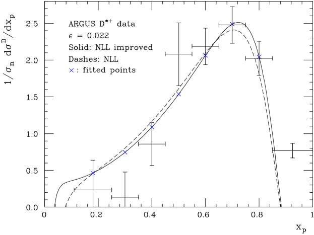
Figure 7: Best fit for the improved fragmentation function at ARGUS. In dashed line, the NLL fragmentation function at the same value of $\epsilon$.

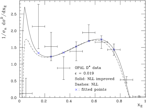
Figure 8: Best fit for the improved fragmentation function at OPAL. In dashed line, the NLL fragmentation function at the same value of $\epsilon$.

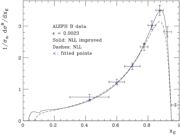
Figure 9: Best fit for the improved fragmentation function at ALEPH. In dashed line, the NLL fragmentation function at the same value of $\epsilon$.

The full improved resummed result of Eq. (5.25) has been used here. For comparison, we have also plotted the NLL curves computed at the same value of $\epsilon$.

In Figs. 11 and 11, we illustrate the NLL differential cross section, obtained with the exponentiated condition (7).

Figure 10: Best fit for the NLL fragmentation function with exponentiated starting condition at ARGUS. In dashed line, the NLL fragmentation function at the same value of $\epsilon$. In dotted line the NLL best fit.

Figure 11: Best fit for the NLL fragmentation function with exponentiated starting condition at OPAL. In dashed line, the NLL fragmentation function at the same value of $\epsilon$. In dotted line the NLL best fit.

We see a better behavior at $x\,\mbox{$\rightarrow$}\,1$, while the values of the $\epsilon$ parameter for the best fit are quite small. For comparison, we have also plotted the NLL curves at the same $\epsilon$ value and the NLL best fit with the value of $\epsilon$ taken from Tab. 2.

The small differences we find in the LL and NLL sectors, with respect to the results of Ref. [3], are due to different range, normalization and adjustment of physical parameters.

From the value of the $\epsilon$ parameter for ARGUS, OPAL and ALEPH, we can easily see that it scales nearly quadratically in the heavy-quark mass, as expected.

8 Conclusions

In this work we have considered the heavy-flavour fragmentation functions in ${e^{+}e^{-}}$ annihilation. We have devised and implemented a method by which all perturbative effects that have been calculated so far can be included in the computation of the fragmentation function. These include leading and next-to-leading logarithmic resummation, fixed-order effects up to ${\cal O}\left(\alpha_{s}^{2}\right)$, and mass effects to the same order.

Our finding can be easily summarized as follows. We generally find little difference between our results and the NLL resummed calculation. This indicates that mass effects are of limited importance in fragmentation-function physics in ${e^{+}e^{-}}$ annihilation. On the other hand, our calculation confirms the fact that, when NLL effects are included, the importance of a non-perturbative initial condition is reduced. For example, at ARGUS energies, we see a strong reduction of the $\epsilon$ parameter, from $0.053$ to $0.018$. This reduction is also observed in the fixed-order calculation, where $\epsilon$ goes from $0.058$ to $0.035$ when the ${\cal O}(\alpha_{s}^{2})$ effects are included.

References

[1]
B. Mele and P. Nason, Nucl. Phys. B361 (1991) 626.
[2]
G. Colangelo and P. Nason, Phys. Lett. B285 (1992) 167.
[3]
M. Cacciari and M. Greco, Phys. Rev. D55 (1997) 7134.
[4]
L. Randall and N. Rius, Nucl. Phys. B441 (1995) 167.
[5]
C. Peterson, D. Schlatter, I. Schmitt and P. M. Zerwas, Phys. Rev. D27 (1983) 105.
[6]
D. Buskulic et al., ALEPH Collaboration, Phys. Lett. B357 (1995) 699.
[7]
G. Alexander et al., OPAL Collaboration, Phys. Lett. B364 (1995) 93.
[8]
K. Abe et al., SLD Collaboration, Phys. Rev. D56 (1997) 5310.
[9]
M. Cacciari, M. Greco and P. Nason, J. High Energy Phys. 05 (1998) 007.
[10]
E. Braaten, K. Cheung, S. Fleming and Tzu Chiang Yuan,
Phys. Rev. D51 (1995) 4819, hep-ph/9409316;
R. L. Jaffe and L. Randall, Nucl. Phys. B412 (1994) 79, hep-ph/9306201.
[11]
P. Nason and C. Oleari, Nucl. Phys. B521 (1998) 237;
C. Oleari, Ph. D. Thesis, hep-ph/9802431.
[12]
G. Rodrigo, Nucl. Phys. Proc. Suppl.54A (1997) 60;
G. Rodrigo, Ph. D. Thesis,
Univ. of València, 1996, hep-ph/9703359;
G. Rodrigo, A. Santamaria and M. Bilenkii, Phys. Rev. Lett. 79 (1997) 193.
[13]
W. Bernreuther, A. Brandenburg and P. Uwer, Phys. Rev. Lett. 79 (1997) 189;
A. Brandenburg and P. Uwer, Nucl. Phys. B515 (1998) 279.
[14]
P. Nason and C. Oleari, Phys. Lett. B418 (1998) 199.
[15]
P. Nason and C. Oleari, Phys. Lett. B447 (1999) 327.
[16]
P. Nason and B. R. Webber, Nucl. Phys. B421 (1994) 473.
[17]
L. J. Reinders, H. Rubinstein and S. Yazaki, Phys. Rep. 127 (1985) 1.
[18] J. Collins, F. Wilczek and A. Zee, Phys. Rev. D18 (1978) 242.
[19]
H. Albrecht et al., ARGUS Collaboration, Z. Phys. C52 (1991) 353.
[20]
R. Akers et al., OPAL Collaboration, Z. Phys. C67 (1995) 27.
[21]
Yu.L. Dokshitzer, V.A. Khoze and S. I. Troyan, Workshop on jet studies at LEP
and HERA, DTP-91/04.
[22]
A. Bassetto, M. Ciafaloni and G. Marchesini, Phys. Rev. 100 (1983) 201.