CERN-TH/99-62

hep-ph/9903513

THE RENORMALIZED GAUGE COUPLING AND
NON-PERTURBATIVE TESTS OF DIMENSIONAL REDUCTION

M. Laine

Theory Division, CERN, CH-1211 Geneva 23, Switzerland
Dept. of Physics, P.O.Box 9, FIN-00014 Univ. of Helsinki, Finland

Abstract

In 4d lattice simulations of Standard Model like theories, the renormalized gauge coupling in the broken phase can be determined from the prefactor of the Yukawa term in the static potential. We compute the same quantity in terms of the conventional $\overline{\mbox{\rm MS}}$ scheme gauge coupling. The result allows for a further non-perturbative test of finite temperature dimensional reduction, by a comparison of the critical temperatures for the electroweak phase transition as obtained with 4d lattice simulations and with 3d effective theory simulations.

CERN-TH/99-62
June 1999

1 Introduction

Consider finite temperature physics at temperatures $\pi T\gg m$, where $m$ stands for the mass scales of the problem. Such a case is for instance the electroweak phase transition at $T_{c}\sim m_{H}/g$, with a Higgs vev $v(T_{c})\sim T_{c}$ [1]. One can then construct a three-dimensional (3d) effective theory for the thermodynamics of the system with the method of dimensional reduction [2]–[5]. The construction is purely perturbative, while the non-perturbative IR-problems of finite temperature field theory are contained in the effective theory. Often, even further degrees of freedom can be integrated out within the 3d theory [2]–[5].

For the electroweak sector of the Standard Model (as well as for many extensions thereof [3]), the final effective action resulting from the procedure described above is of the very simple form

$$S_{\mbox{\scriptsize eff}}=\int d^{3}x\biggl{[}{1\over 4}F_{ij}^{a}F_{ij}^{a}+{1\over 4}B_{ij}B_{ij}+(D_{i}\phi)^{\dagger}D_{i}\phi+m_{3}^{2}\phi^{\dagger}\phi+\lambda_{3}(\phi^{\dagger}\phi)^{2}\biggr{]},$$ (1)

where $F_{ij}^{a}$ and $B_{ij}$ are the SU(2) and U(1) field strength tensors. The dynamics of this theory depends on the SU(2) and U(1) gauge couplings $g_{3}^{2},g_{3}^{\prime 2}$, as well as on the Higgs sector parameters $m_{3}^{2},\lambda_{3}$ (or, more precisely, on the three dimensionless ratios that can be formed thereof). The practical content of dimensional reduction is to compute these parameters as a perturbative expansion in the underlying physical 4d parameters and the temperature; explicit derivations have been carried out in [3, 6]. For instance, the expression for $m_{3}^{2}$ is parametrically of the form

$$m_{3}^{2}=m^{2}(\bar{\mu})\Bigl{[}1+{\cal O}(g^{2})\Bigr{]}+g^{2}(\bar{\mu})T^{2}\Bigl{[}1+{\cal O}(g)+{\cal O}(g^{2})\Bigr{]},$$ (2)

where the parameters appearing on the right hand side are those of the corresponding 4d theory in the $\overline{\mbox{\rm MS}}$ scheme (see below), with $\bar{\mu}$ the $\overline{\mbox{\rm MS}}$ scale parameter, and all the leading ${\cal O}(g,g^{2})$ corrections shown have been explicitly computed for several theories.

Of course, the final 3d theory obtained with dimensional reduction, such as the one in Eq. (1), is “only” an effective theory, and it is not arbitrarily precise. Analytically, the accuracy of dimensional reduction can be estimated by considering the set of one-particle-irreducible Green’s functions for the degrees of freedom contained in Eq. (1), and comparing the effects of the higher-dimensional operators left out from the effective theory, with those arising within the effective theory. The conclusion is that the relative error remaining in the non-vanishing P- and CP-even static bosonic Green’s functions with “soft” external momenta is highly suppressed, ${\cal O}(g^{3})$, already when only super-renormalizable operators are kept in the effective theory [3] (as is the case with Eq. (1)). Numerically, the error was estimated to be at the percent level for the Standard Model (the largest corrections arising from the top loops, and from the Matsubara zero modes of the temporal components of the gauge fields) [3].

However, many of the quantities addressed with the effective theory are purely non-perturbative. Thus, it is strictly speaking impossible to estimate the numerical accuracy analytically. Even though it is clear that the non-perturbative effects can only arise from the degrees of freedom contained in the 3d theory, one may still ask what the relative accuracy obtained is for such quantities. While in the electroweak case this is not feasible within the full Standard Model due to chiral fermions, the question can at least be addressed within the SU(2)+Higgs model with 4d finite temperature lattice simulations (the U(1) subgroup is not too essential for these considerations [7]).

The 4d simulations relevant for studying the accuracy of the theory in Eq. (1), have been carried out with a gauge coupling which is $\sim$50% larger than the physical one, $g^{2}\approx 0.585$ [8, 9]. This should increase the possible discrepancies. However, the system still has multiple length scales ($\sim\pi T,gT,g^{2}T$), making the extrapolation of the 4d results to the continuum limit extremely demanding (but unavoidable if one wants to compare with the 3d theory). Consequently, the extrapolation has been carried out in the full range of relevant Higgs masses only very recently [9].

The problem we study here is a systematic comparison of the 4d lattice results in [8, 9] with the 3d effective theory results in [7, 10]. In order to make such a comparison, we will need to perform one further (well convergent) zero temperature perturbative computation, to which we now turn.

2 Formulation of the problem

Dropping chiral fermions and the U(1) subgroup from the standard electroweak theory, we consider the 4d SU(2)+Higgs model in this paper:

$$S=\int d^{4}x\biggl{[}{\frac{1}{4}}F^{a}_{\mu\nu}F^{a}_{\mu\nu}+(D_{\mu}\phi)^{\dagger}(D_{\mu}\phi)+m^{2}\phi^{\dagger}\phi+\lambda(\phi^{\dagger}\phi)^{2}\biggr{]},$$ (3)

where $D_{\mu}=\partial_{\mu}+igT^{a}A^{a}_{\mu}$. The theory in Eq. (3) has three parameters: the scalar mass parameter $m^{2}$, the scalar self-coupling $\lambda$ and the gauge coupling $g^{2}$. To fix a particular physical theory, one has to choose a regularization scheme and then give the values of the renormalized couplings in this scheme in terms of some physical quantities. As a regularization scheme we choose $\overline{\mbox{\rm MS}}$ as is convenient in continuum computations, and in particular in dimensional reduction [3]. The question we address then is, what are the values of the $\overline{\mbox{\rm MS}}$ parameters if a set of physical observables is determined, either by experiment or by 4d lattice simulations?

In the broken phase of the theory, two of the $\overline{\mbox{\rm MS}}$ couplings can then be fixed in terms of the physical masses of the Higgs and the W boson, $m_{H}$ and $m_{W}$, respectively:

$$m^{2}(\bar{\mu})=-{\frac{1}{2}}m_{H}^{2}+\delta m^{2}(\bar{\mu}),\quad\lambda(\bar{\mu})=\frac{g^{2}(\bar{\mu})}{8}\frac{m_{H}^{2}}{m_{W}^{2}}+\delta\lambda(\bar{\mu}),$$ (4)

where the 1-loop corrections $\delta m^{2}(\bar{\mu}),\delta\lambda(\bar{\mu})$ are easily computable (we employ here the formulas given in [3]). However, the value of the gauge coupling $g^{2}(\bar{\mu})$ cannot be fixed in terms of the masses. In the physical case with fermions, $g^{2}(\bar{\mu})$ can be fixed, e.g., through the muon lifetime; for an explicit expression see Eq. (183) in [3]. However, this is not available in the theory of Eq. (3).

We thus need another physical observable sensitive to $g^{2}$. Moreover, since we are ultimately interested in lattice studies of the theory in Eq. (3), this observable should be measurable in Monte Carlo simulations. A suitable choice is the “renormalized gauge coupling $g_{R}^{2}$” [12]. The value of $g_{R}^{2}$ is obtained from the static potential $V(r)$: from a large rectangular Wilson loop $W(r,t)$ of size $r\times t$ (in Euclidian space), one determines

$$V(r)=\lim_{t\to\infty}-\frac{1}{t}\ln W(r,t).$$ (5)

At leading order, the potential thus defined is

$$V_{\mbox{\scriptsize tree}}(r)=-g^{2}C_{F}\int\frac{d^{3}p}{(2\pi)^{3}}\frac{e^{i{\bf p}\cdot{\bf r}}-1}{p^{2}+m_{W}^{2}}=-g^{2}C_{F}\frac{e^{-m_{W}r}}{4\pi r}+V_{\mbox{\scriptsize tree}}(\infty),$$ (6)

where $C_{F}=(N^{2}-1)/(2N)=3/4$ and $V_{\mbox{\scriptsize tree}}(\infty)$ is a regularization dependent constant. Let us now define

$$g_{R}^{2}(r)=\frac{1}{C_{F}}\frac{\frac{d}{dr}\Bigl{[}-V(r)\Bigr{]}}{\frac{d}{dr}\int\frac{d^{3}p}{(2\pi)^{3}}\frac{e^{i{\bf p}\cdot{\bf r}}}{p^{2}+M^{2}}},$$ (7)

where $M$ is some physical mass parameter, chosen in [12, 8] to be the measured coefficient of the exponential falloff of $V(r)$. At leading order, $M$ coincides with $m_{W}$. In [8, 9], the distance used in $g_{R}^{2}(r)$ was further fixed to be $r=M^{-1}$. Note that the choice of $M$ in the dominator of Eq. (7) has a 1st order effect on $g_{R}^{2}$, $\delta g_{R}^{2}\propto g^{2}(\delta M/M)$, while the choice of $r$ has only a 2nd order effect, $\delta g_{R}^{2}\propto g^{2}(\delta r/r)^{2}$ (see below).

The expression in Eq. (7) is the continuum version of the definition given in [12]: we do not discuss the finite lattice spacing artifacts, but assume that the extrapolation to the continuum limit performed in [8] is reliable. To leading order, the result of the definition in Eq. (7) is just $g^{2}(\bar{\mu})$, but $g_{R}^{2}(M^{-1})$ is defined also fully non-perturbatively.

Our objective is now to find the relation of $g^{2}(\bar{\mu})$ and $g_{R}^{2}(M^{-1})$ at 1-loop level (for clarity, we often denote $g^{2}(\bar{\mu})=g^{2}_{\mbox{\scriptsize$\overline{\mbox{\rm MS}}$}}(\bar{\mu})$). Both quantities are finite and not sensitive to the ultraviolet regularization, so that the computation can be carried out in the continuum. In this way, we have found the $\overline{\mbox{\rm MS}}$ parameters to which the 4d simulations correspond (Sec. 3). The $\overline{\mbox{\rm MS}}$ parameters are, in turn, the input in dimensional reduction and the construction of 3d effective theories, so that with the relation found, we can compare the results of direct 4d finite temperature lattice simulations with those of 3d effective theory simulations (Sec. 4).

Finally, it should be mentioned that there is also another approach available for determining the $\overline{\mbox{\rm MS}}$ scheme parameters to which the 4d simulations correspond. Indeed, instead of going via a set of physical observables, one could directly relate the bare lattice parameters at a finite but small lattice spacing $a$, and the renormalized $\overline{\mbox{\rm MS}}$ parameters, as first done for QCD in [13]. In the continuum limit the end results of the two approaches are in principle equivalent up to higher order effects. However, the convergence properties can be somewhat different: relating the regularization schemes is a computation only sensitive to the ultraviolet, while the computation we carry out is only sensitive to the infrared. The reason why we choose our approach is that the extrapolation to the continuum limit has in [8, 9] been carried out directly for the physical observables $m_{H},m_{W},g_{R}^{2}$, so that this way we get rid of any reference to a finite lattice spacing, as is necessary for a comparison of 4d and 3d lattice results. The 1-loop computation we perform is very well convergent despite the infrared sensitivity, since we are in the broken phase of the theory. It should be noted, though, that for the academic case of very small Higgs masses close to the Coleman-Weinberg limit $m_{H}\approx 10$ GeV, the “strict loop expansion” formulas [3] we employ here for relating $m_{H},m_{W}$ to $m^{2}(\bar{\mu}),\lambda(\bar{\mu})$ break down (see Sec. 4).

3 Computation of $g_{R}^{2}$

Preliminaries. We carry out the computation in a general ’t Hooft $R_{\xi}$-gauge with the gauge parameter $\xi$ and, for the moment, a general spacetime dimension $d$. We denote the different structure constants appearing as

$$(T^{a}T^{a})_{ij}=C_{F}\delta_{ij},\quad f^{abc}f^{abd}=C_{A}\delta^{cd},\quad T^{a}T^{b}T^{a}T^{b}=C_{F}^{2}-{\frac{1}{2}}C_{F}C_{A},$$ (8)

where $C_{F}=(N^{2}-1)/(2N),C_{A}=N$. The actual computation is carried out for $N=2$, but we keep the symbols $C_{F},C_{A}$ in some of the formulas below, to differentiate between two classes of contributions (Abelian and non-Abelian; see the Appendix).

The object we compute is the expectation value of a rectangular Wilson loop in the limit $t\to\infty$, Eq. (5). It can be seen that the horizontal parts of the path ($t=$ const.) do not contribute in this limit [14, 15]. Thus, denoting

$$U(-{\bf r}/2,t)={\cal P}\exp\Bigl{[}ig\int_{-t/2}^{t/2}dt^{\prime}T^{a}A^{a}_{0}(-{\bf r}/2,t^{\prime})\Bigr{]},$$ (9)

where the path-ordered exponential is defined through

$${\cal P}\exp\Bigl{[}\int_{-T}^{T}dt^{\prime}M(t^{\prime})\Bigr{]}=1+\int_{-T}^{T}dt^{\prime}M(t^{\prime})+\int_{-T}^{T}dt^{\prime}dt^{\prime\prime}\theta(t^{\prime}-t^{\prime\prime})M(t^{\prime\prime})M(t^{\prime})+\ldots,$$ (10)

the expectation value to be computed is

$$\lim_{t\to\infty}W(r,t)=\lim_{t\to\infty}\langle U(-{\bf r}/2,t)U^{\dagger}({\bf r}/2,t)\rangle.$$ (11)

The actual computation proceeds in a straightforward way, by inserting the expansion in Eq. (10) into Eq. (11). The $\theta$-functions can be written as usual as

$$\theta(t)=\int\frac{d\omega}{2\pi}\frac{e^{i\omega t}}{i\omega+\epsilon^{+}}.$$ (12)

The $t^{\prime}$-integral in Eq. (9) makes the sources static in the limit $t\to\infty$, and in momentum ($\omega$) space, the graphs then produce a term linear in $t$ via

$$2\pi\delta(0)\to t.$$ (13)

Through Eq. (5), the coefficient of the linear term gives $-V(r)$. This computation is, of course, a direct generalization of the one in [14] for QCD (for 2-loop results in QCD, see [15]). The graphs needed are shown in Fig. 1, and the results for these individual graphs are given in the Appendix.

Figure 1: The graphs contributing to the static potential at 1-loop level. “Mirror” configurations are not shown. Graph (g) is a counterterm contribution.

The loop contributions. The final result for the computation of the graphs in Fig. 1 can be expressed in terms of the functions

$$A_{0}(m^{2}) = \int\frac{d^{d}p}{(2\pi)^{d}}\frac{1}{p^{2}+m^{2}},$$ (14)

$$B_{0}(k^{2};m_{1}^{2},m_{2}^{2}) = \int\frac{d^{d}p}{(2\pi)^{d}}\frac{1}{[p^{2}+m_{1}^{2}][(p+k)^{2}+m_{2}^{2}]}.$$ (15)

Summing all the graphs together, we obtain (for $N=2$)

$$-V_{\mbox{\scriptsize 1-loop}}(r)=g^{4}C_{F}C_{A}\int\frac{d^{d-1}p}{(2\pi)^{d-1}}\frac{e^{i{\bf p}\cdot{\bf r}}}{p^{2}+m_{W}^{2}}\biggl{\{}$$

$$\hskip 28.45274pt2B_{0}(0;m_{W}^{2},m_{W}^{2})+(p^{2}+m_{W}^{2})\frac{d}{dm_{W}^{2}}B_{0}(p^{2};m_{W}^{2},m_{W}^{2})$$

$$\hskip 28.45274pt+\frac{1}{8(d-1)(p^{2}+m_{W}^{2})}\biggl{[}B_{0}(p^{2};m_{W}^{2},m_{W}^{2})\Bigl{(}3(4d-3){p^{2}}+12(3-2d){m_{W}^{2}}\Bigr{)}$$

$$\hskip 28.45274pt-B_{0}(p^{2};m_{W}^{2},m_{H}^{2})\frac{1}{p^{2}}\Bigl{(}{p^{4}}+(6-4d){p^{2}}{m_{W}^{2}}+2p^{2}{m_{H}^{2}}+({m_{W}^{2}}-{m_{H}^{2}})^{2}\Bigr{)}$$

$$\hskip 28.45274pt+A_{0}(m_{W}^{2})\frac{1}{p^{2}m_{H}^{2}}\Bigl{(}6{{(d-1)}^{2}}{p^{2}}{m_{W}^{2}}-p^{2}m_{H}^{2}(29-32d+8{d^{2}})+{m_{H}^{4}}-{m_{H}^{2}}m_{W}^{2}\Bigr{)}$$

$$\hskip 28.45274pt+A_{0}(m_{H}^{2})\frac{1}{p^{2}}\Bigl{(}(2d-1)p^{2}+m_{W}^{2}-{m_{H}^{2}}\Bigr{)}\biggl{]}+\,{\rm counterterms}\biggr{\}}.$$ (16)

This result is, of course, independent of the gauge parameter $\xi$, even though the single contributions given in the Appendix do depend on it.

Specializing then to $d=4-2\epsilon$, $A_{0},B_{0}$ have their standard forms

$$A_{0}(m^{2})\!\! = \!\!-\frac{\mu^{-2\epsilon}}{(4\pi)^{2}}m^{2}\left(\frac{1}{\epsilon}+\ln\frac{\bar{\mu}^{2}}{m^{2}}+1\right),$$ (17)

$$B_{0}(k^{2};m_{1}^{2},m_{2}^{2})\!\! = \!\!\frac{\mu^{-2\epsilon}}{(4\pi)^{2}}\biggl{[}\frac{1}{\epsilon}+\ln\frac{\bar{\mu}^{2}}{m_{1}m_{2}}+1-\frac{m_{1}^{2}+m_{2}^{2}}{m_{1}^{2}-m_{2}^{2}}\ln\frac{m_{1}}{m_{2}}+F_{E}(k^{2};m_{1}^{2},m_{2}^{2})\biggr{]},\mbox{\hskip 22.76228pt}$$ (18)

where

$$F_{E}(k^{2};m_{1}^{2},m_{2}^{2})=1+\frac{m_{1}^{2}+m_{2}^{2}}{m_{1}^{2}-m_{2}^{2}}\ln\frac{m_{1}}{m_{2}}+\frac{m_{1}^{2}-m_{2}^{2}}{k^{2}}\ln\frac{m_{1}}{m_{2}}$$

$$\hskip 28.45274pt+\frac{1}{k^{2}}\sqrt{(m_{1}+m_{2})^{2}+k^{2}}\sqrt{(m_{1}-m_{2})^{2}+k^{2}}\ln\frac{1-\sqrt{\frac{(m_{1}-m_{2})^{2}+k^{2}}{(m_{1}+m_{2})^{2}+k^{2}}}}{1+\sqrt{\frac{(m_{1}-m_{2})^{2}+k^{2}}{(m_{1}+m_{2})^{2}+k^{2}}}}.$$ (19)

Including also the counterterms which cancel the $1/\epsilon$ divergences, we obtain

$$-V_{\mbox{\scriptsize 1-loop}}(r) = \frac{g^{4}}{16\pi^{2}}C_{F}C_{A}\int\frac{d^{3}p}{(2\pi)^{3}}\frac{e^{i{\bf p}\cdot{\bf r}}}{p^{2}+m_{W}^{2}}\biggl{\{}$$ (20)

$$\frac{p^{2}+m_{W}^{2}}{p^{2}}\frac{2}{\sqrt{1+\frac{4m_{W}^{2}}{p^{2}}}}\ln\frac{1-(1+\frac{4m_{W}^{2}}{p^{2}})^{-1/2}}{1+(1+\frac{4m_{W}^{2}}{p^{2}})^{-1/2}}$$

$$+ \frac{1}{p^{2}+m_{W}^{2}}\biggl{[}\frac{1}{24h^{2}}\Bigl{(}86{h^{2}}{p^{2}}-9(6-3h^{2}+{h^{4}}){m_{W}^{2}}\Bigr{)}\ln\frac{\bar{\mu}^{2}}{m_{W}^{2}}$$

$$+ {\frac{1}{8}}(13{p^{2}}-20{m_{W}^{2}})F_{E}(p^{2};m_{W}^{2},m_{W}^{2})$$

$$- \frac{1}{24}\Bigl{(}(h^{2}-1)^{2}\frac{m_{W}^{4}}{p^{2}}+{p^{2}}+2(h^{2}-5){m_{W}^{2}}\Bigr{)}F_{E}(p^{2};m_{W}^{2},m_{H}^{2})$$

$$+ \frac{h^{2}\ln h}{12(h^{2}-1)}\Bigl{(}{p^{2}}+(9{h^{2}}-17){m_{W}^{2}}\Bigr{)}$$

$$+ \frac{1}{72h^{2}}\Bigl{(}{h^{2}}{p^{2}}+3(-18+{h^{2}}-11{h^{4}}){m_{W}^{2}}\Bigr{)}\biggr{]}\biggr{\}},$$

where $h=m_{H}/m_{W}$.

The Fourier transformation. It remains to evaluate Eq. (7), i.e., to take the derivative with respect to $r$ and to perform the final integral with respect to ${\bf p}$. Let us note here that since the difference between $M$ and $m_{W}^{\mbox{\scriptsize tree}}$ is of relative order $g^{2}$ and the scale dependence of $g^{2}_{\mbox{\scriptsize$\overline{\mbox{\rm MS}}$}}(\bar{\mu})$ is already of order $g^{4}$, we can replace $M^{-1}$ by $(m_{W}^{\mbox{\scriptsize tree}})^{-1}$ in the argument of $g_{R}^{2}(r)$ in the present 1-loop computation. For the time being we denote the tree-level value of the W mass by $m_{W}=m_{W}^{\mbox{\scriptsize tree}}$. Within 1-loop corrections, the difference between $m_{W}^{\mbox{\scriptsize tree}}$ and $m_{W}^{\mbox{\scriptsize 1-loop}}$ is naturally of higher order.

Figure 2: The integration contour in the $p_{z}$-plane.

The final ${\bf p}$-integral to be evaluated is convergent and can be done numerically by brute force, but it can be put in a more illuminating and rapidly convergent form by doing a part of it by contours. We write ${\bf p}=(p_{z},{\bf p}_{\perp})$, such that ${\bf p}\cdot{\bf r}=p_{z}r$, and close the $p_{z}$-integral in the upper half plane. The analytic structure of the $p_{z}$-integrand is that there is a (1st or 2nd order) pole at $p_{z}=+i({p}_{\perp}^{2}+m_{W}^{2})$, and cuts along the imaginary axis starting at some $p_{z}=ip_{z}^{0}$, see Fig. 2.

The pole contribution. The pole contribution is of the form

$$\left.\frac{d}{dr}\int\frac{d^{3}p}{(2\pi)^{3}}\frac{e^{ip_{z}r}}{(p^{2}+m_{W}^{2})^{2}}{\cal F}(p^{2}+m_{W}^{2})\right|_{r=m_{W}^{-1}}=-\frac{1}{8\pi}e^{-1}\Bigl{[}{\cal F}(0)+4{\cal F}^{\prime}(0)m_{W}^{2}\Bigr{]}.$$ (21)

For the expression in the square brackets in Eq. (20) (the term on the 2nd row in Eq. (20) does not contribute),

$${\cal F}(0) = m_{W}^{2}\biggl{[}\left(-{\frac{59}{24}}-{\frac{9}{{4h^{2}}}}-\frac{3}{8}{h^{2}}\right)\ln\frac{\bar{\mu}^{2}}{m_{W}^{2}}$$ (22)

$$- \frac{h}{12}\left(12-4{h^{2}}+{h^{4}}\right)\sqrt{4-h^{2}}\arctan{\sqrt{{\frac{2-h}{2+h}}}}$$

$$- \frac{1}{24}{h^{4}}({h^{2}-6})\ln h+\frac{1}{72h^{2}}\left(-54+{h^{2}}(-556+99{\sqrt{3}}\pi)-45{h^{4}}+3{h^{6}}\right)\biggr{]}$$

$$= -{\frac{1}{2}}\biggl{(}\frac{g^{2}}{(4\pi)^{2}}\biggr{)}^{-1}\delta m_{W}^{2{\rm(1-loop)}},$$

$${\cal F}^{\prime}(0) = {\frac{43}{12}}\ln\frac{\bar{\mu}^{2}}{m_{W}^{2}}$$ (23)

$$+ \frac{h}{12\sqrt{4-h^{2}}}\left(-36+32{h^{2}}-13{h^{4}}+2{h^{6}}\right)\arctan{\sqrt{{\frac{2-h}{2+h}}}}$$

$$+ \frac{1}{24}\left(12-18{h^{2}}+9{h^{4}}-2{h^{6}}\right)\ln h-\frac{1}{72}(26+18{h^{2}}-6{h^{4}}-27{\sqrt{3}}\pi).$$

In Eq. (22), $m_{W}^{2}+\delta m_{W}^{2{\rm(1-loop)}}$ denotes the 1-loop W pole mass squared.

The cut contribution. The cut contribution is of the form

$$\int_{-\infty}^{\infty}dp_{z}{\cal F}(p_{z})\to\int_{p_{z}^{0}}^{\infty}idp_{z}\Bigl{[}{\cal F}(ip_{z}+\epsilon)-{\cal F}(ip_{z}-\epsilon)\Bigr{]}=-2\int_{p_{z}^{0}}^{\infty}dp_{z}\mathop{\mbox{Im}}{\cal F}(ip_{z}+\epsilon).$$ (24)

Non-vanishing imaginary parts arise from the function $F_{E}(p^{2};m_{1}^{2},m_{2}^{2})$ in Eq. (19), and from the first logarithm in Eq. (20):

$$\left.\mathop{\mbox{Im}}F_{E}(p^{2};m_{1}^{2},m_{2}^{2})\right|_{p_{z}\to ip_{z}+\epsilon}=-\theta(p_{z}^{2}-p_{\perp}^{2}-(m_{1}+m_{2})^{2})$$

$$\hskip 28.45274pt\times\frac{\pi}{p_{z}^{2}-p_{\perp}^{2}}\sqrt{p_{z}^{2}-p_{\perp}^{2}-(m_{1}+m_{2})^{2}}\sqrt{p_{z}^{2}-p_{\perp}^{2}-(m_{1}-m_{2})^{2}},$$ (25)

$$\mathop{\mbox{Im}}\left.\frac{2}{p^{2}\sqrt{1+\frac{4m_{W}^{2}}{p^{2}}}}\ln\frac{1-(1+\frac{4m_{W}^{2}}{p^{2}})^{-1/2}}{1+(1+\frac{4m_{W}^{2}}{p^{2}})^{-1/2}}\right|_{p_{z}\to ip_{z}+\epsilon}$$

$$\hskip 28.45274pt=\theta(p_{z}^{2}-p_{\perp}^{2}-4m_{W}^{2})\frac{2\pi}{p_{z}^{2}-p_{\perp}^{2}}\frac{1}{\sqrt{1-\frac{4m_{W}^{2}}{p_{z}^{2}-p_{\perp}^{2}}}}.$$ (26)

The expression in the curly brackets in Eq. (20) then contributes as follows: from the first term and from $F_{E}(p^{2};m_{W}^{2},m_{W}^{2})$, one gets a constant factor which, by a change of variables, can be written in the following rapidly convergent form:

$$f_{0}=\int_{2}^{\infty}\!dy\int_{0}^{\infty}\!dze^{-(y+z)}y\left(y+z\right)$$

$$\hskip 28.45274pt\times\frac{144+336yz+168{z^{2}}+116{y^{2}}{z^{2}}+116y{z^{3}}+29{z^{4}}}{4\left(3+2yz+{z^{2}}\right)^{2}\sqrt{z\left(2y+z\right)\left(4+2yz+{z^{2}}\right)}}=2.156946.$$ (27)

From $F_{E}(p^{2};m_{W}^{2},m_{H}^{2})$, on the other hand, there is a contribution which depends on $h$; it can be similarly written, e.g., in the form

$$f(h)\!\! = \!\!-\int_{h+1}^{\infty}\!dy\int_{0}^{\infty}\!dze^{-(y+z)}\frac{y\left(y+z\right)\sqrt{z\left(2y+z\right)\left(4h+2yz+{z^{2}}\right)}}{12\left[(h+1)^{2}+2yz+{z^{2}}\right]^{2}\left[h(h+2)+2yz+{z^{2}}\right]^{2}}$$ (28)

$$\times\left(z^{4}+4yz^{3}+4y^{2}z^{2}+4(h+3)z^{2}+8(h+3)yz+12(h+1)^{2}\right).$$

The numerical values of $f(h)$ are given in Table 1 and Fig. 3.

The final result. We are now in a position to collect all the terms together, to evaluate Eq. (7). The denominator there gives, to 1st order in $M-m_{W}\propto g^{2}$,

$$\left.\frac{d}{dr}\frac{1}{4\pi r}\exp\Bigl{(}-Mr\Bigr{)}\right|_{r=m_{W}^{-1}}=-\frac{1}{2\pi}e^{-1}m_{W}^{2}\biggl{(}1+{\frac{1}{2}}\frac{m_{W}-M}{m_{W}}\biggr{)}.$$ (29)

The order $(m_{W}-M)$ term here combines with ${\cal F}(0)$ in Eqs. (21), (22), to replace $m_{W}$ with $m_{W}^{\mbox{\scriptsize 1-loop}}$. The final result left is then

$$g_{R}^{2}(M^{-1}) = g^{2}_{\mbox{\scriptsize$\overline{\mbox{\rm MS}}$}}(\bar{\mu})\biggl{(}1+{\frac{1}{2}}\frac{M-m_{W}}{m_{W}}\biggr{)}+\frac{g^{4}}{(4\pi)^{2}}\Bigl{[}2{\cal F}^{\prime}(0)-e\Bigl{(}f_{0}+f(h)\Bigr{)}\Bigr{]}$$ (30)

$$\equiv g^{2}_{\mbox{\scriptsize$\overline{\mbox{\rm MS}}$}}(m_{W})\biggl{(}1+{\frac{1}{2}}\frac{M-m_{W}}{m_{W}}\biggr{)}+\frac{g^{4}_{\mbox{\scriptsize$\overline{\mbox{\rm MS}}$}}(m_{W})}{(4\pi)^{2}}C(h),$$

where ${\cal F}^{\prime}(0)$, $f_{0}$, $f(h)$ are from Eqs. (23), (27), (28), and we have now restored the meaning of $m_{W}$ as the physical (1-loop) pole mass. Going from the first to the second row in Eq. (30), we have merged the first term of ${\cal F}^{\prime}(0)$ in Eq. (23) with $g^{2}_{\mbox{\scriptsize$\overline{\mbox{\rm MS}}$}}(\bar{\mu})$, which produces $g^{2}_{\mbox{\scriptsize$\overline{\mbox{\rm MS}}$}}(m_{W})$ up to corrections which are of higher order than the present computation, and we have then chosen to use the same scale also in all the terms of order $g^{4}_{\mbox{\scriptsize$\overline{\mbox{\rm MS}}$}}$, again by ignoring terms which are of higher order. After this replacement, only the latter two rows in Eq. (23) contribute on the latter row in Eq. (30):

$$C(h)=\left.2{\cal F}^{\prime}(0)\right|_{\bar{\mu}=m_{W}}-e\Bigl{(}f_{0}+f(h)\Bigr{)}.$$ (31)

The numerical values of $C(h)$ are shown in Table 1 and Fig. 3. While $f(h)$ diverges logarithmically at small $h$, $C(h)$ is finite.

$h$	$f(h)$	$C(h)$
0.2	-0.249947	-3.78735
0.4	-0.118355	-3.69862
0.6	-0.0660750	-3.62889
0.8	-0.0399324	-3.57204
1.0	-0.0253292	-3.52459
1.2	-0.0166083	-3.48430
1.4	-0.0111594	-3.44959
1.6	-0.00764098	-3.41935
1.8	-0.00531146	-3.39272
2.0	-0.00373821	-3.36907

Table 1: The values of $f(h)$ and $C(h)$, Eqs. (28), (30), at selected values of $h$.

Figure 3: The functions $f(h)$ and $C(h)$ from Eqs. (28), (30).

The fact that $C(h)$ is negative, means that $g^{2}_{\mbox{\scriptsize$\overline{\mbox{\rm MS}}$}}(m_{W})$ tends to be larger than $g_{R}^{2}(M^{-1})$. If $M$, $m_{W}$, $m_{H}$ and $g_{R}^{2}(M^{-1})$ have been measured as in [8, 9], then

$$g^{2}_{\mbox{\scriptsize$\overline{\mbox{\rm MS}}$}}(m_{W})\approx g_{R}^{2}(M^{-1})\biggl{(}1+{\frac{1}{2}}\frac{m_{W}-M}{m_{W}}\biggr{)}+\frac{|C(m_{H}/m_{W})|}{158}g_{R}^{4}(M^{-1}).$$ (32)

This relation constitutes our main result.

4 Implications for dimensional reduction

As we recall from Sec. 1, in the finite temperature case one is mainly interested in comparing results for non-perturbative quantities between the 4d and 3d approaches. One of the non-perturbative quantities addressed is the critical Higgs mass of the electroweak phase diagram. The phase diagram contains a line of first order phase transitions, which ends at a certain Higgs mass $m_{H,c}$ [10],[16]-[20]. A comparison of the 4d and 3d results for $m_{H,c}$ yields perfect agreement at the percent level [9]. This comparison was possible even before the relation of $g_{R}^{2}$ and $g_{\mbox{\scriptsize$\overline{\mbox{\rm MS}}$}}^{2}$ was known, since it turns out that $m_{H,c}$ depends only very weakly on $g_{\mbox{\scriptsize$\overline{\mbox{\rm MS}}$}}^{2}$ [21] (see also Fig. 4).

Here we perform a comparison for another quantity, the critical temperature $T_{c}$. This comparison is in principle less powerful than that for $m_{H,c}$, since both the leading ($T_{c}\sim m_{H}/g$) and next-to-leading ($\delta T_{c}\sim m_{H}/(4\pi)$) contributions are perturbative [22] and thus definitely agree within the 4d and 3d theories. However, starting from the next-to-next-to-leading order ($\delta T_{c}\sim gm_{H}/(4\pi)^{2}$), $T_{c}$ is non-perturbative [22]. (These statements can be easily understood from Eqs. (2),(4). Apart from perturbative terms within the 3d theory in Eq. (1), the critical point is where $m_{3}^{2}=cg_{3}^{4}=c(g^{2}T)^{2}$, where $c$ is a non-perturbative coefficient which can only be determined numerically.) Since $T_{c}$ can be measured with good accuracy with lattice simulations, a comparison becomes meaningful. Due to the strong dependence on $g$, $T_{c}\sim m_{H}/g$, the relation of the $g_{R}^{2}$ determined with 4d simulations and the $g^{2}_{\mbox{\scriptsize$\overline{\mbox{\rm MS}}$}}$ used in the 3d theory, is necessary for such a comparison: it is only sensible to discuss a non-perturbative effect of relative order ${\cal O}(g^{2})$, once a perturbative ambiguity of the same relative order has been removed by the computation carried out in this paper.

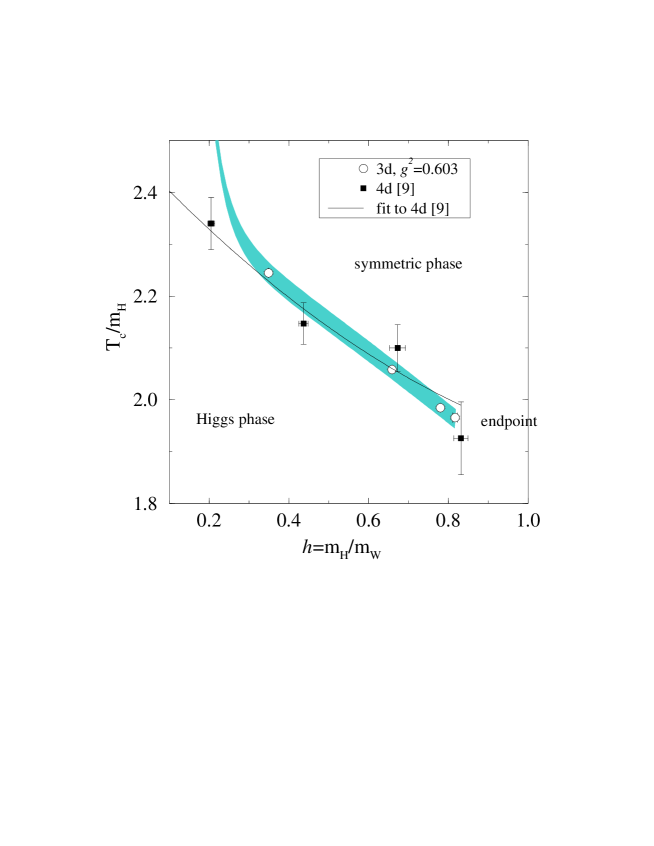
Figure 4: A comparison of the phase diagrams obtained with 4d and 3d simulations. The 4d results are from [9], and the 3d results from [7, 10, 21]. The gray band has been obtained by subtracting from the 3d lattice values the 3d perturbative values, fitting a curve to the difference, adding the perturbative curve (which is very accurate within 3d at small $h$), and then converting to 4d physical units according to the formulas in [3]. The coupling was varied in the interval $g^{2}_{\mbox{\scriptsize$\overline{\mbox{\rm MS}}$}}(m_{W})=0.603\pm 0.012$, the smallest $g^{2}_{\mbox{\scriptsize$\overline{\mbox{\rm MS}}$}}$ corresponding to the upper edge of the band. The discrepancy at small $h$ is mainly due to the fact that the relation of $m_{H},m_{W}$ to $m^{2}(\bar{\mu}),\lambda(\bar{\mu})$ employed here and taken from [3], starts to break down as one approaches the Coleman-Weinberg limit $h\sim 0.13$, but also to the fact that the 3d theory itself is less accurate at small $h$ since the high-temperature expansion is not applicable in the case of an extremely strong transition.

With 4d lattice simulations, the continuum extrapolation for $T_{c}$ has been determined for $m_{H}=34$ GeV in [8], and for some other values, in particular $m_{H}=m_{H,c}$, in [9]. The corresponding gauge coupling was measured to be $g_{R}^{2}(M^{-1})=0.585(10)$ at $m_{H}=34$ GeV and, we interpret, consistent with this at $m_{H}=m_{H,c}$ [9]. The mass parameter $M$ was observed to be close to the physical W mass $m_{W}$, but from Tables 4,5 in [8], we observe that there is a small discrepancy which, giving more weight to the lattices closest to the continuum limit ($L_{t}=4,5$), we estimate as $(m_{W}-M)/m_{W}\approx 0.035(25)$. We now see from Eq. (32) that this leads to $g_{\mbox{\scriptsize$\overline{\mbox{\rm MS}}$}}^{2}(m_{W})\approx 0.603(12)$. With this value, we can convert the 3d results [7, 10, 21] to be comparable with the 4d results, as explained in [11]. The result is shown in Fig. 4.

We conclude that the phase transition line $T_{c}(m_{H})$, and in particular $m_{H,c}$, $T_{c}(m_{H,c})$, are in perfect agreement within statistical errors at least for $h\mathop{\raise 1.29167pt\hbox{$>$\kern-7.5pt\raise-4.73611pt\hbox{$\sim$}}}0.3$ ($m_{H}\mathop{\raise 1.29167pt\hbox{$>$\kern-7.5pt\raise-4.73611pt\hbox{$\sim$}}}25$ GeV), whether determined directly from 4d or from a 3d effective theory. For smaller $h$, the vacuum renormalization employed [3] in relating $m_{H},m_{W}$ to $\overline{\mbox{\rm MS}}$ scheme breaks down, but even there dimensional reduction and the 3d theory themselves are not completely off in spite of the very strong transition, as we have checked separately by a vacuum renormalization which is accurate at the Coleman-Weinberg point $h\approx 0.13$: we get there $T_{c}/m_{H}\approx 2.5$. Thus, dimensional reduction seems indeed as effective as one would have expected from the analytical estimates.

5 Conclusions

In this paper, we have carried out a perturbative 1-loop computation in the broken phase of the 4d SU(2)+Higgs theory, which establishes a relation between the “renormalized gauge coupling” determined by measuring the static potential with lattice Monte Carlo simulations, and the conventional $\overline{\mbox{\rm MS}}$ scheme gauge coupling $g^{2}(\bar{\mu})$. With existing results for the mass parameter $m^{2}(\bar{\mu})$ and scalar self-coupling $\lambda(\bar{\mu})$, this relation completes what is needed for a reliable comparison of 4d simulation results, and analytical computations where the $\overline{\mbox{\rm MS}}$ scheme is a natural starting point. As an important application, we have considered the accuracy of finite temperature dimensional reduction, which is used, e.g., in the context of 3d effective theory studies of the electroweak phase transition.

The conclusion we find for dimensional reduction and the resulting 3d effective field theory is that, even for the non-perturbative characteristics of the electroweak phase transition, the numerical accuracy is consistent with what it was analytically estimated to be, i.e., at the percent level. This is quite good since, from the point of view of electroweak baryogenesis, studying the electroweak phase transition with 3d effective theories and lattice simulations continues to be phenomenologically interesting in many extensions of the Standard Model, such as the MSSM [24].

Note added

I thank Y. Schröder for pointing out that Eq. (16) agrees, for $N=2$, with the general result obtained for SU($N$)+Higgs in [25].

Very recently, a preprint appeared [26] where the same problem is addressed as in Sec. 3 of the present paper.

Appendix Appendix

In this Appendix, we show the results for the individual graphs in Fig. 1. The results are given as contributions to the coefficient of $t$ in $\ln W(r,t)$, Eq. (11), and they are thus contributions to $-V(r)$ according to Eq. (5). We leave out a common factor

$$g^{4}C_{F}C_{A}\int\frac{d^{d-1}p}{(2\pi)^{d-1}}\frac{e^{i{\bf p}\cdot{\bf r}}}{{p}^{2}+m_{W}^{2}}$$ (33)

from all the non-Abelian terms (i.e., those proportional to $C_{F}C_{A}$). The Abelian terms (i.e., those proportional to $C_{F}^{2}$) only contribute to the exponentiation of the leading order result in Eq. (6): they always come with the coefficient ${\frac{1}{2}}t^{2}$ in $W(r,t)$ (see [14, 15] for a more precise discussion). Note that the explicit counterterm contribution, graph (g) in Fig. 1, comes from the bare combination

$$g_{B}A_{B}=\biggl{(}1-\frac{g^{2}\mu^{-2\epsilon}}{(4\pi)^{2}\epsilon}\frac{3+\xi}{4}C_{A}\biggr{)}gA,$$ (34)

where the numerical value is given for $d=4-2\epsilon$.

The contributions of the different graphs are:

$$\mbox{(a)}+\left.\mbox{(b)}\right|_{\mbox{\scriptsize Abel.\ part}}=\mbox{exponentiation of the $r$-dependent term of Eq.~{}(\ref{Vtree})},$$ (35)

$$\left.\mbox{(b)}\right|_{\mbox{\scriptsize non-Abel.\ part}}=(p^{2}+m_{W}^{2})\frac{dB_{0}(p^{2};m_{W}^{2},m_{W}^{2})}{dm_{W}^{2}}$$

$$\hskip 28.45274pt+\frac{p^{2}+m_{W}^{2}}{8(d-1)p^{2}m_{W}^{4}}\biggl{\{}-B_{0}(p^{2},\xi m_{W}^{2},\xi m_{W}^{2})p^{2}(p^{2}+4\xi m_{W}^{2})$$

$$\hskip 28.45274pt+2B_{0}(p^{2};m_{W}^{2},\xi m_{W}^{2})\Bigl{[}p^{4}+2p^{2}m_{W}^{2}(3+\xi-2d)+m_{W}^{4}(\xi-1)^{2}\Bigr{]}$$

$$\hskip 28.45274pt-B_{0}(p^{2};m_{W}^{2},m_{W}^{2})p^{2}\Bigl{[}p^{2}+4(3-2d)m_{W}^{2}\Bigr{]}$$

$$\hskip 28.45274pt+2m_{W}^{2}(\xi-1)\Bigl{[}A_{0}(\xi m_{W}^{2})-A_{0}(m_{W}^{2})\Bigr{]}\biggr{\}},$$ (36)

$$\mbox{(c)}+\left.\mbox{(d)}\right|_{\mbox{\scriptsize Abel.\ part}}=\mbox{exponentiation containing the cross-term from Eq.~{}(\ref{Vtree}),\hskip 34.14322pt}$$ (37)

$$\left.\mbox{(d)}\right|_{\mbox{\scriptsize non-Abel.\ part}}=2B_{0}(0;m_{W}^{2},m_{W}^{2})+\frac{1}{m_{W}^{2}}\Bigl{[}A_{0}(\xi m_{W}^{2})-A_{0}(m_{W}^{2})\Bigr{]},$$ (38)

$$\mbox{(e)}=\frac{1}{4(d-1)m_{W}^{4}p^{2}}\biggl{\{}B_{0}(p^{2},\xi m_{W}^{2},\xi m_{W}^{2})p^{4}\left({p^{2}}+4\xi{m_{W}^{2}}\right)$$

$$\hskip 28.45274pt-2B_{0}(p^{2};m_{W}^{2},\xi m_{W}^{2})(p^{2}+{m_{W}^{2}})\Bigl{[}{p^{4}}+2{p^{2}}{m_{W}^{2}}\left(3+\xi-2d\right)+{m_{W}^{4}}{{\left(\xi-1\right)}^{2}}\Bigr{]}$$

$$\hskip 28.45274pt+B_{0}(p^{2};m_{W}^{2},m_{W}^{2})p^{2}\Bigl{[}{p^{4}}+2\left(7-4d\right)p^{2}{m_{W}^{2}}+8\left(2-d\right){m_{W}^{4}}\Bigr{]}$$

$$\hskip 28.45274pt+2m_{W}^{2}\Bigl{[}A_{0}(m_{W}^{2})-A_{0}(\xi m_{W}^{2})\Bigr{]}\left[{p^{2}}\left(4d-6+\xi\right)+{m_{W}^{2}}\left(\xi-1\right)\right]\biggr{\}},$$ (39)

$$\mbox{(f)}=\frac{-\Pi_{W}(p^{2})}{C_{A}(p^{2}+m_{W}^{2})}=\mbox{Eq.~{}(\ref{res1})}-\left.\mbox{(b)}\right|_{\mbox{\scriptsize non-Abel.\ part}}-\left.\mbox{(d)}\right|_{\mbox{\scriptsize non-Abel.\ part}}-\mbox{(e)}$$

$$\hskip 28.45274pt-\,\Bigl{\{}\mbox{all $1/\epsilon$-divergences}\Bigr{\}},$$ (40)

$$\mbox{(g)}=-\frac{3+\xi}{2}\frac{\mu^{-2\epsilon}}{(4\pi)^{2}\epsilon}.$$ (41)

References

- [1] V.A. Rubakov and M.E. Shaposhnikov, Usp. Fiz. Nauk 166 (1996) 493 [hep-ph/9603208].
- [2] P. Ginsparg, Nucl. Phys. B 170 (1980) 388; T. Appelquist and R. Pisarski, Phys. Rev. D 23 (1981) 2305.
- [3] K. Kajantie, M. Laine, K. Rummukainen and M. Shaposhnikov, Nucl. Phys. B 458 (1996) 90 [hep-ph/9508379]; Phys. Lett. B 423 (1998) 137 [hep-ph/9710538].
- [4] E. Braaten and A. Nieto, Phys. Rev. D 53 (1996) 3421 [hep-ph/9510408].
- [5] A. Jakovác and A. Patkós, Nucl. Phys. B 494 (1997) 54 [hep-ph/9609364].
- [6] M. Laine, Nucl. Phys. B 481 (1996) 43 [hep-ph/9605283]; J.M. Cline and K. Kainulainen, Nucl. Phys. B 482 (1996) 73 [hep-ph/9605235]; Nucl. Phys. B 510 (1997) 88 [hep-ph/9705201]; M. Losada, Phys. Rev. D 56 (1997) 2893 [hep-ph/9605266]; G.R. Farrar and M. Losada, Phys. Lett. B 406 (1997) 60 [hep-ph/9612346].
- [7] K. Kajantie, M. Laine, K. Rummukainen and M. Shaposhnikov, Nucl. Phys. B 466 (1996) 189 [hep-lat/9510020]; Nucl. Phys. B 493 (1997) 413 [hep-lat/9612006].
- [8] F. Csikor, Z. Fodor, J. Hein, A. Jaster and I. Montvay, Nucl. Phys. B 474 (1996) 421 [hep-lat/9601016].
- [9] F. Csikor, Z. Fodor and J. Heitger, Phys. Rev. Lett. 82 (1999) 21 [hep-ph/9809291].
- [10] K. Kajantie, M. Laine, K. Rummukainen and M. Shaposhnikov, Phys. Rev. Lett. 77 (1996) 2887 [hep-ph/9605288]; K. Rummukainen, M. Tsypin, K. Kajantie, M. Laine and M. Shaposhnikov, Nucl. Phys. B 532 (1998) 283 [hep-lat/9805013].
- [11] M. Laine, Phys. Lett. B 385 (1996) 249 [hep-lat/9604011].
- [12] Z. Fodor, J. Hein, K. Jansen, A. Jaster and I. Montvay, Nucl. Phys. B 439 (1995) 147 [hep-lat/9409017].
- [13] A. Hasenfratz and P. Hasenfratz, Phys. Lett. B 93 (1980) 165; R. Dashen and D.J. Gross, Phys. Rev. D 23 (1981) 2340.
- [14] W. Fischler, Nucl. Phys. B 129 (1977) 157.
- [15] M. Peter, Phys. Rev. Lett. 78 (1997) 602 [hep-ph/9610209]; Nucl. Phys. B 501 (1997) 471 [hep-ph/9702245]; Y. Schröder, Phys. Lett. B 447 (1999) 321 [hep-ph/9812205].
- [16] F. Karsch, T. Neuhaus, A. Patkós and J. Rank, Nucl. Phys. B (Proc. Suppl.) 53 (1997) 623 [hep-lat/9608087].
- [17] M. Gürtler, E.-M. Ilgenfritz and A. Schiller, Phys. Rev. D 56 (1997) 3888 [hep-lat/9704013]; E.-M. Ilgenfritz, A. Schiller and C. Strecha, hep-lat/9807023.
- [18] O. Philipsen, M. Teper and H. Wittig, Nucl. Phys. B 528 (1998) 379 [hep-lat/9709145].
- [19] Y. Aoki, Phys. Rev. D 56 (1997) 3860 [hep-lat/9612023]; Y. Aoki, F. Csikor, Z. Fodor and A. Ukawa, hep-lat/9901021.
- [20] F. Csikor, Z. Fodor and J. Heitger, Phys. Lett. B 441 (1998) 354 [hep-lat/9807021].
- [21] M. Laine and K. Rummukainen, to appear in the Proceedings of Lattice ’98, July 1998, Boulder, Colorado [hep-lat/9809045].
- [22] P. Arnold, Phys. Rev. D 46 (1992) 2628 [hep-ph/9204228].
- [23] K. Jansen and M. Laine, Phys. Lett. B 435 (1998) 166 [hep-lat/9805024].
- [24] D. Bödeker, P. John, M. Laine and M.G. Schmidt, Nucl. Phys. B 497 (1997) 387 [hep-ph/9612364]; M. Laine and K. Rummukainen, Phys. Rev. Lett. 80 (1998) 5259 [hep-ph/9804255]; Nucl. Phys. B 535 (1998) 423 [hep-lat/9804019]; Nucl. Phys. B 545 (1999) 141 [hep-ph/9811369]; M. Losada, Nucl. Phys. B 537 (1999) 3 [hep-ph/9806519]; hep-ph/9905441.
- [25] Y. Schröder, PhD thesis, DESY, Hamburg, 1999 (unpublished).
- [26] F. Csikor, Z. Fodor, P. Hegedüs and A. Piróth, hep-ph/9906260.