Renormalization Group Improved Heavy Quark Production in Polarized $\gamma\gamma$ Collisions
Michael Melles¹ and W. James Stirling^1,2
1) Department of Physics, University of Durham, Durham DH1 3LE, U.K.

2) Department of Mathematical Sciences, University of Durham, Durham DH1 3LE, U.K.

Abstract

The experimental determination of the partial width $\Gamma(H\longrightarrow\gamma\gamma)$ of an intermediate mass Higgs is among the most important measurements at a future photon photon collider. Recently it was shown that large non-Sudakov as well as Sudakov double logarithmic (DL) corrections can be summed to all orders in the background process $\gamma\gamma\,(J_{z}=0)\longrightarrow q\overline{q}$. It was found that positivity and stability of the cross section was only restored at the four-loop level. One remaining large source of uncertainty stems from the fact that the scale of the strong coupling is unspecified within the double logarithmic approximation. In this paper we include the leading and next-to-leading order running coupling to all orders. We thus remove the inherent scale uncertainty of both the exact one-loop and all-orders DL result without encountering any Landau-pole singularities. The effect is significant and, for the non-Sudakov form factor, is found to correspond to an effective scale of roughly $\alpha_{s}(9m_{q}^{2})$.

1 Introduction

The model independent knowledge of the total Higgs width combined with respective branching ratios allows an experimental determination of various partial widths of the Higgs boson [1, 2]. It is therefore of fundamental importance for a detailed understanding of the electroweak symmetry breaking mechanism. For an intermediate mass Higgs, i.e. with a mass below the $W^{+}W^{-}$ threshold (in the MSSM mass window), a photon linear collider (PLC) offers so far the only possibility of a direct and model independent measurement of $\Gamma_{tot}$. Using Compton backscattering [3, 4, 5] of initially polarized electrons and positrons the partial width $\Gamma(H\longrightarrow\gamma\gamma)$ can be determined with very good precision at a PLC [6]. This quantity is of significant interest in its own right, since all charged massive particles contribute in the loop which might therefore be sensitive to new physics. With the respective branching ratio BR$(H\longrightarrow\gamma\gamma)$, determined in measurements at the LHC (and possibly also the NLC), the total width can be reconstructed.

The dominant non-Higgs background for this energy regime is $\gamma\gamma(J_{z}=0)\longrightarrow q\overline{q}$ with $q=b,c$. While this background is suppressed by $\frac{m_{q}^{2}}{s}$ at the Born level (unlike the $J_{z}=\pm 2$ channel), higher-order QCD radiative (Bremsstrahlung) corrections in principle remove this suppression [7]. In addition, large virtual non-Sudakov double $\log(s/m_{q}^{2})$ logarithms (DL) are present which at one loop can even lead to a negative cross section [8, 9]. In Ref. [10] we presented explicit three-loop results in the DL approximation which revealed a factorization of hard (non-Sudakov) and soft (Sudakov) double logarithms for this process and led to the all-orders resummation in the form of a confluent hypergeometric function ${}_{2}F_{2}$:

$$\sigma^{DL}_{{\rm virt}+{\rm soft}} = \sigma_{\rm Born}\left\{1+{\cal F}\;\;_{2}F_{2}(1,1;2,\frac{3}{2};\frac{1}{2}{\cal F})+2\;{\cal F}\;\;_{2}F_{2}(1,1;2,\frac{3}{2};\frac{C_{A}}{4C_{F}}{\cal F})\right\}^{2}$$ (1)

$$\exp\left(\frac{\alpha_{s}C_{F}}{\pi}\left[\log\frac{s}{m_{q}^{2}}\left(\frac{1}{2}-\log\frac{s}{4l_{c}^{2}}\right)+\log\frac{s}{4l_{c}^{2}}-1+\frac{\pi^{2}}{3}\right]\right)$$

where ${\cal F}=-C_{F}\frac{\alpha_{s}}{4\pi}\log^{2}\frac{s}{m^{2}}$ is the one-loop hard form factor. The Born cross section is given by

$$\frac{d\sigma_{\rm Born}}{d\cos\theta}\left(\gamma+\gamma(J_{z}=0)\longrightarrow q+\overline{q}\right)=\frac{12\pi\alpha^{2}Q_{q}^{4}}{s}\frac{\beta\left(1-\beta^{4}\right)}{\left(1-\beta^{2}\cos^{2}\theta\right)^{2}}$$ (2)

where $\beta=\sqrt{1-\frac{4m_{q}^{2}}{s}}$ denotes the quark velocity and $Q_{q}$ the charge of the quark with mass $m_{q}$. $\alpha=\frac{1}{137}$ is the fine structure constant and $\sqrt{s}$ the center-of-mass energy of the initial photons.

In Ref. [11] it was pointed out that one needs to include at least four loops (at the cross section level) of the non-Sudakov hard logarithms in order to achieve positivity and stability. A major source of uncertainty remained in the scale choice of the QCD coupling, two possible ‘natural’ choices — $\alpha_{s}(s)$ and $\alpha_{s}(m_{q}^{2})$ — yielding very different numerical results.

In this work we include the exact leading and next-to-leading order running coupling into the derivation of both the massive Sudakov and the novel hard (non-Sudakov) form factors, thus removing a major source of error in both the exact one-loop and all-orders DL results. Our technique is based on the observation that in a particular loop in a multi-loop ladder, the correct scale for the strong coupling is the characteristic transverse momentum flowing round the loop. Details are given in Section 2. In Section 3 we present numerical results including the full one-loop radiative corrections based on Refs. [7] and [8] with the new renormalization group improved form factor. Section 4 contains our conclusions.

2 Renormalization Group Improved Form Factors

In this section we will include the QCD running coupling into the DL form factors given in Eq. 1. A very important result incorporated in this expression for the virtual plus soft real Bremsstrahlung cross section is the factorization between Sudakov and non-Sudakov double logarithms [10]. For our purposes here this means that it is sufficient to consider the corrections for the basic topologies shown in Fig. 1 separately. The complete RG improved result is then given by the same factorized structure.

Within the DL approximation the scale at which to evaluate the QCD coupling is unspecified, and this is therefore a major source of uncertainty in the determination of the size of the $b\overline{b}$, $c\overline{c}$ background for intermediate mass Higgs production. In the following we will derive the renormalization group effect of inserting a running coupling into each loop evaluation using the exact one- and two-loop solution of the $\beta$-function. All higher-order RG-terms will then be suppressed by $\frac{1}{\log^{3}\frac{s}{m^{2}}}$. We begin with the more familiar case of topology $A$ (see Fig. 1).

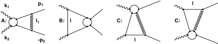
Figure 1: The schematic one-loop soft (Sudakov,“A”) and hard (non-Sudakov,“B,C”) topologies contributing to the DL form factor. These graphs are obtained from the one-loop box diagram in the process $\gamma\gamma(J_{z}=0)\longrightarrow q\overline{q}$. The blob denotes a hard momentum flowing through the omitted propagator relative to the soft momentum $l$ or $l_{1}$ in the DL phase space. For higher-order DL contributions, only corrections to these topologies need to be taken into account.

2.1 The Sudakov RG-Form Factor

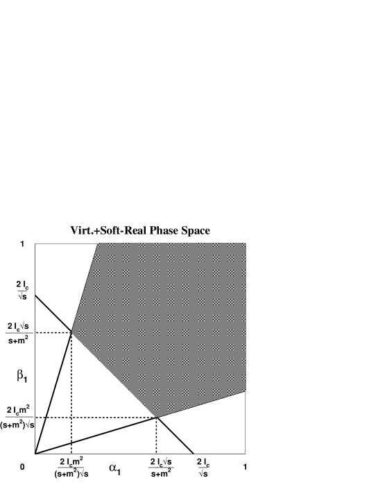
Figure 2: The schematic DL-phase space for the massive virtual (upper diagram) and the virtual plus soft real Sudakov form factor (lower diagram). The sum is gluon mass independent for $\lambda<\frac{2l_{c}m}{\sqrt{s}}$.

Figure 3: A schematic Feynman diagram leading to the Sudakov double logarithms in the process $\gamma\gamma(J_{z}=0)\longrightarrow q\overline{q}$ with $i$ gluon insertions. The blob denotes a hard momentum going through the omitted propagator in the DL-phase space. Crossed diagrams lead to a different ordering of the Sudakov variables with all resulting $C_{A}$ terms canceling the DL-contributions from three gluon insertions [10]. The scale of the coupling $\alpha_{s}=\frac{g_{s}^{2}}{4\pi}$ is indicated at the vertices and explicitly taken into account in this work.

In the derivation of the leading logarithmic corrections in Ref. [10] we used the familiar Sudakov technique [13, 14, 15] of decomposing loop momenta into components along external momenta, denoted by $\{\alpha,\beta\}$, and those perpendicular to them, denoted by $l_{\perp}$. For massless fermions, the effective scale for Sudakov double logarithms for the coupling at each loop is $\alpha_{s}({\bf l^{2}_{\perp}})$, as was shown in Refs. [16, 17, 18] by direct comparison with explicit higher-order calculations. For massive fermions the effective scale is also given by ${\bf l^{2}_{\perp}}\equiv-l^{2}_{\perp}>0$ as the dominant double logarithmic phase space is given by $\frac{m^{2}}{s}\ll\frac{{\bf l^{2}_{\perp}}}{s}\ll 1$ [10] (on a formal DL level, setting $m=\lambda$ yields the massless Sudakov form factor). We start by writing

$$\alpha_{s}({\bf l^{2}_{\perp}})=\frac{\alpha_{s}(m^{2})}{1+\beta_{0}\frac{\alpha_{s}(m^{2})}{\pi}\log\frac{{\bf l^{2}_{\perp}}}{m^{2}}+\beta_{1}\left(\frac{\alpha_{s}(m^{2})}{\pi}\right)^{2}\log\frac{{\bf l^{2}_{\perp}}}{m^{2}}}\equiv\frac{\alpha_{s}(m^{2})}{1+c\;\log\frac{{\bf l^{2}_{\perp}}}{m^{2}}}$$ (3)

where $\beta_{0}=\frac{11}{12}C_{A}-\frac{4}{12}T_{F}n_{F}$, $\beta_{1}=\frac{17}{24}C_{A}^{2}-\frac{5}{12}C_{A}T_{F}n_{F}-\frac{1}{4}C_{F}T_{F}n_{F}$ and for QCD we have $C_{A}=3$, $C_{F}=\frac{4}{3}$ and $T_{F}=\frac{1}{2}$ as usual. Up to two loops the massless $\beta$-function is independent of the chosen renormalization scheme and is gauge invariant in minimally subtracted schemes to all orders [12]. These features will also hold for the derived renormalization group improved form factors below.

In case of the Sudakov DL’s, the DL-phase space structure is very transparent in terms of the $\{\alpha_{1},\beta_{1}\}$ parameters. This is shown in Fig. 2 for the virtual and virtual plus soft real Bremsstrahlung phase space. We therefore use the on-shell condition ${\bf l^{2}_{1_{\perp}}}=s\alpha_{1}\beta_{1}$, even though the running coupling will now depend on two integration variables.

The DL result for the virtual one-loop Sudakov form factor can be written in terms of integrals over $\alpha_{1}$ and $\beta_{1}$ as:

$${\cal F}^{DL}_{S_{V}} = -\frac{\alpha_{s}C_{F}}{2\pi}\int^{1}_{0}\frac{d\beta_{1}}{\beta_{1}}\int^{1}_{0}\frac{d\alpha_{1}}{\alpha_{1}}\Theta(s\alpha_{1}\beta_{1}-\lambda^{2})\Theta(\alpha_{1}-\frac{m^{2}}{s}\beta_{1})\Theta(\beta_{1}-\frac{m^{2}}{s}\alpha_{1})$$ (4)

$$= -\frac{\alpha_{s}C_{F}}{2\pi}\left(\frac{1}{2}\log^{2}\frac{s}{m^{2}}+\log\frac{s}{m^{2}}\log\frac{m^{2}}{\lambda^{2}}\right)\;.$$

Here $\lambda$ is a fictitious gluon mass introduced to regulate the infra-red divergences in the real and virtual gluon integrals. For the inclusion of double logarithms from the real Bremsstrahlung contribution we introduce a cutoff for the energy integration according to $\lambda\leq l_{0}\leq l_{c}$, i.e. in terms of Sudakov variables, $\alpha_{1}+\beta_{1}\leq\frac{l_{c}}{E_{\rm cm}}=\frac{2l_{c}}{\sqrt{s}}$. Thus we find for the real DL Bremsstrahlung contribution:

$${\cal F}^{DL}_{S_{R}} = \frac{\alpha_{s}C_{F}}{\pi}\int^{1}_{0}\frac{d\beta_{1}}{\beta_{1}}\int^{1}_{0}\frac{d\alpha_{1}}{\alpha_{1}}\Theta(s\alpha_{1}\beta_{1}-\lambda^{2})\Theta(\alpha_{1}-\frac{m^{2}}{s}\beta_{1})\Theta(\beta_{1}-\frac{m^{2}}{s}\alpha_{1})$$ (5)

$$\times\Theta\left(\frac{2l_{c}}{\sqrt{s}}-\alpha_{1}-\beta_{1}\right)$$

$$= -2{\cal F}^{DL}_{S_{V}}-\frac{\alpha_{s}C_{F}}{\pi}\int^{1}_{0}\frac{d\beta_{1}}{\beta_{1}}\int^{1}_{0}\frac{d\alpha_{1}}{\alpha_{1}}\Theta(\alpha_{1}-\frac{m^{2}}{s}\beta_{1})\Theta(\beta_{1}-\frac{m^{2}}{s}\alpha_{1})$$

$$\times\Theta\left(\alpha_{1}+\beta_{1}-\frac{2l_{c}}{\sqrt{s}}\right)$$

$$= \frac{\alpha_{s}C_{F}}{\pi}\left(\frac{1}{2}\log^{2}\frac{s}{m^{2}}+\log\frac{s}{m^{2}}\log\frac{m^{2}}{\lambda^{2}}-\log\frac{s}{m^{2}}\log\frac{s}{4l_{c}^{2}}\right)$$

assuming only $\lambda<\frac{2l_{c}m}{\sqrt{s}}$. These results are of course well known [13, 15, 11] but now can be used to insert a running coupling into each loop integration. The DL result is sufficient for this purpose as the RG-logarithms are sub-leading at the next order in $\alpha_{s}$. At this point we only give the result for the sum ${\cal F}^{DL}_{S_{R}}+2{\cal F}^{DL}_{S_{V}}$, as only this combination is relevant for a physical cross section. We emphasize at this point that in a adopting a certain jet definition, we need to make sure that it does not restrict the exponentiation of the energy cut dependent piece of the soft gluon matrix elemtent. In the Appendix we give the result for the renormalization group improved ${\cal F}^{DL}_{S_{V}}$ form factor and in addition the two-loop results, thus checking the requirement that all one-loop RG-form factors exponentiate. We find

$${\cal F}^{RG}_{S_{R}}+2{\cal F}^{RG}_{S_{V}} = -\frac{C_{F}}{\pi}\left\{\int_{\frac{2l_{c}m^{2}}{(s+m^{2})\sqrt{s}}}^{\frac{2l_{c}\sqrt{s}}{s+m^{2}}}\frac{d\beta_{1}}{\beta_{1}}\int^{1}_{\frac{2l_{c}}{\sqrt{s}}-\beta_{1}}\frac{d\alpha_{1}}{\alpha_{1}}+\int^{1}_{\frac{2l_{c}}{\sqrt{s}}}\frac{d\beta_{1}}{\beta_{1}}\int^{1}_{\frac{m^{2}}{s}\beta_{1}}\frac{d\alpha_{1}}{\alpha_{1}}\right.$$ (6)

$$\left.-\int_{\frac{2l_{c}m^{2}}{s\sqrt{s}}}^{\frac{m^{2}}{s}}\frac{d\beta_{1}}{\beta_{1}}\int^{1}_{\frac{s}{m^{2}}\beta_{1}}\frac{d\alpha_{1}}{\alpha_{1}}\right\}\frac{\alpha_{s}(m^{2})}{1+c\;\log\frac{s\alpha_{1}\beta_{1}}{m^{2}}}$$

$$= -\frac{\alpha_{s}(m^{2})C_{F}}{\pi\;c}\left\{-\int_{\frac{2l_{c}m^{2}}{(s+m^{2})\sqrt{s}}}^{\frac{2l_{c}\sqrt{s}}{s+m^{2}}}\frac{d\beta_{1}}{\beta_{1}}\log\frac{1+c\;\log\left(\left(\frac{2l_{c}}{\sqrt{s}}-\beta_{1}\right)\beta_{1}\frac{s}{m^{2}}\right)}{\left(1+c\;\log\frac{s\beta_{1}}{m^{2}}\right)}\right.$$

$$+\log\frac{s}{m^{2}}\log\frac{\alpha_{s}(2l_{c}\sqrt{s})}{\alpha_{s}(s)}+\log\frac{2l_{c}}{\sqrt{s}}\log\frac{\alpha_{s}(2l_{c}\sqrt{s})}{\alpha_{s}\left(\frac{2l_{c}m^{2}}{\sqrt{s}}\right)}$$

$$\left.+\frac{1}{c}\log\frac{\alpha_{s}(m^{2})\alpha_{s}(2l_{c}\sqrt{s})}{\alpha_{s}(s)\alpha_{s}\left(\frac{2l_{c}m^{2}}{\sqrt{s}}\right)}\right\}\;.$$

An expansion in $\alpha_{s}(m^{2})$ gives the double logarithmic result plus subleading terms in $\beta_{0}$ etc. The dependence on the cutoff $l_{c}$ will vanish when the hard-gluon Bremsstrahlung contributions are added order by order. Fig. 4 compares the second term in the exponential obtained from the renormalization group improved result in Eq. 6 with the explicit two-loop result given in Eq. 25 of the Appendix. We emphasize that the two loop result depends on two “running” scales , ${\bf l_{1_{\perp}}}$ and ${\bf l_{2_{\perp}}}$. The figure clearly shows that our one-loop result exponentiates as expected.

Figure 4: The second term in the exponential obtained from the renormalization group improved massive one-loop Sudakov form factor compared with the explicit two-loop results given in the appendix. The latter depends on a different scale in each loop integration. The quark mass is kept fixed at $m_{b}=4.5$ GeV and the values for the real gluon energy cutoff $l_{c}$ is indicated in the figure. The result in Eq. 6 clearly exponentiates.

Since in this work we are only able to include the hard one-gluon matrix elements (the exact NNLO corrections are presently unknown), the higher-order terms are at this point of a more academic interest. Our two jet definition (see below) restricts the higher-order hard gluon radiation phase space sufficiently so that it is reasonable to neglect more than one gluon emission. As mentioned above, Fig. 4 shows, using explicit RG-improved two loop DL-results in the Appendix, that the result in Eq. 6 exponentiates as expected. We do have to consider the subleading terms already entering at the one-loop level as the hard Bremsstrahlung contribution will also contain subleading terms in $l_{c}$. The complete result for the renormalization group improved massive Sudakov form factor is thus given by:

$$\widetilde{{\cal F}}^{RG}_{S_{R}}+2\widetilde{{\cal F}}^{RG}_{S_{V}} = \frac{\alpha_{s}(m^{2})C_{F}}{\pi}\left\{\frac{1}{c}\int_{\frac{2l_{c}m^{2}}{(s+m^{2})\sqrt{s}}}^{\frac{2l_{c}\sqrt{s}}{s+m^{2}}}\frac{d\beta_{1}}{\beta_{1}}\log\frac{1+c\;\log\left(\left(\frac{2l_{c}}{\sqrt{s}}-\beta_{1}\right)\beta_{1}\frac{s}{m^{2}}\right)}{\left(1+c\;\log\frac{s\beta_{1}}{m^{2}}\right)}\right.$$ (7)

$$-\frac{1}{c}\log\frac{s}{m^{2}}\log\frac{\alpha_{s}(2l_{c}\sqrt{s})}{\alpha_{s}(s)}-\frac{1}{c}\log\frac{2l_{c}}{\sqrt{s}}\log\frac{\alpha_{s}(2l_{c}\sqrt{s})}{\alpha_{s}\left(\frac{2l_{c}m^{2}}{\sqrt{s}}\right)}$$

$$\left.-\frac{1}{c^{2}}\log\frac{\alpha_{s}(m^{2})\alpha_{s}(2l_{c}\sqrt{s})}{\alpha_{s}(s)\alpha_{s}\left(\frac{2l_{c}m^{2}}{\sqrt{s}}\right)}+\frac{1}{2}\log\frac{s}{m^{2}}+\log\frac{s}{4l_{c}^{2}}-1+\frac{\pi^{2}}{3}\right\}\;,$$

assuming only $\frac{m^{2}}{s}\ll 1$. Expanding in $\alpha_{s}(m^{2})$ gives the DL-Sudakov form factor in Eq. 1 together with subleading terms proportional to $\beta_{0}$ and subsubleading terms proportional to $\beta_{1}$. We emphasize that the two-loop running coupling is included in Eq. 7 to all orders and that all collinear divergences are avoided due to the fact that we keep all non-homogeneous fermion mass terms. We next turn to the virtual hard DL corrections and investigate the RG effects for these contributions.

2.2 The Non-Sudakov RG-Form Factor

In the absence of exact two-loop QCD corrections to the process $\gamma\gamma(J_{z}=0)\longrightarrow q\overline{q}$ it might seem unclear how to perform a renormalization group improvement for the hard non-Sudakov DL’s. We find, however, following similar arguments as in the case of the massive Sudakov DL’s of the previous section, that the same effective scale ${\bf l^{2}_{\perp}}$ is also valid for the novel non-Sudakov logarithms which were summed to give the confluent hypergeometric function ${}_{2}F_{2}$ in Ref. [10]. One way to see this is to note that on a formal level, all insertions of gluons into the hard topology shown in Fig. 5 have the same structure as in the Sudakov case. Only the last fermion loop integration separates the two cases by effectively regularizing soft divergences with the quark mass. The strong coupling receives no renormalization from this last integration so that the scales of the couplings at each order are determined by the same renormalization group arguments as for the Sudakov case. In this context it is worth pointing out that our analysis here also thus removes the largest uncertainty in the exact one-loop calculation of Ref. [8], as the scale of $\alpha_{s}$ in that work was unspecified at this order.

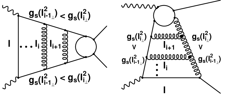
Figure 5: The schematic Feynman diagrams leading to the hard (non-Sudakov) double logarithms in the process $\gamma\gamma(J_{z}=0)\longrightarrow q\overline{q}$ with $i+1$ gluon insertions. The blobs denote a hard momentum going through the omitted propagator in the DL-phase space. Crossed diagrams lead to a different ordering of the Sudakov variables and are correctly accounted for by a factor of $(i+1)!$ at each order. The scale of the coupling $\alpha_{s}=\frac{g_{s}^{2}}{4\pi}$ is indicated at the vertices and included explicitly in this work. The topology on the left-hand diagram is Abelian like, and the one on the right is non-Abelian beyond one loop.

From the exact next-to-leading order result for the running coupling in Eq. 3 it is clear that a formulation in terms of ${\bf l^{2}_{\perp}}$ of the series leading to the non-Sudakov double logarithms is more adaptable to a renormalization group improvement. In Ref. [10] these contributions were derived by first integrating over all $l^{2}_{\perp}$ with integrals over $\{\alpha,\beta\}$ pairs remaining. For the topology depicted on the left in Fig. 5 we find that it can be reformulated as follows:

$${\cal F}\;_{2}F_{2}(1,1;2,\frac{3}{2};\frac{1}{2}{\cal F})\!\!\! = \!\!\!\!\sum^{\infty}_{n=1}\int^{1}_{\frac{m^{2}}{s}}\frac{d\alpha}{\alpha}\int^{1}_{\frac{m^{2}}{s\alpha}}\frac{d\beta}{\beta}\prod^{n-2}_{i=0}\Gamma(n)\!\!\int^{1}_{\alpha_{i}}\frac{d\alpha_{i+1}}{\alpha_{i+1}}\int^{1}_{\beta_{i}}\frac{d\beta_{i+1}}{\beta_{i+1}}\left(\frac{-\alpha_{s}C_{F}}{2\pi}\right)^{n}$$ (8)

$$= \!\!\!\!\sum^{\infty}_{n=1}\int^{s}_{m^{2}}\frac{d{\bf l^{2}_{\perp}}}{{\bf l^{2}_{\perp}}}\int^{1}_{\frac{{\bf l^{2}_{\perp}}}{s}}\frac{d\alpha}{\alpha}\prod^{n-2}_{i=0}\Gamma(n)\!\!\int^{{\bf l^{2}_{i_{\perp}}}}_{m^{2}}\!\frac{d{\bf l^{2}_{{i+1}_{\perp}}}}{{\bf l^{2}_{{i+1}_{\perp}}}}\int^{1}_{\alpha_{i}}\frac{d\alpha_{i+1}}{\alpha_{i+1}}\left(\frac{-\alpha_{s}C_{F}}{2\pi}\right)^{n}$$

where ${\cal F}=-\frac{\alpha_{s}C_{F}}{4\pi}\log^{2}\frac{s}{m^{2}}$ denotes the hard one-loop form factor of Ref. [10]. In this result the product is set to one for $n=1$, and contains nested integrals for $n\geq 2$ with ${\bf l^{2}_{0_{\perp}}}\equiv{\bf l^{2}_{\perp}}$ and $\alpha_{0}\equiv\alpha$. From this expression it is clear that an incorporation of the running coupling in Eq. 3 will not contain any Landau pole singularity [19] as $m^{2}\leq{\bf l^{2}_{i_{\perp}}}\leq{\bf l^{2}_{\perp}}$. We now include the running of $\alpha_{s}$ according to Eq. 3 as follows. For each gluon insertion we have

$$\int^{{\bf l^{2}_{i_{\perp}}}}_{m^{2}}\frac{d{\bf l^{2}_{{i+1}_{\perp}}}}{{\bf l^{2}_{{i+1}_{\perp}}}}\int^{1}_{\alpha_{i}}\frac{d\alpha_{i+1}}{\alpha_{i+1}}\frac{\alpha_{s}(m^{2})}{1+c\;\log\frac{{\bf l^{2}_{{i+1}_{\perp}}}}{m^{2}}} = -\frac{\alpha_{s}(m^{2})}{c}\log\alpha_{i}\log(1+c\;\log\frac{{\bf l^{2}_{i_{\perp}}}}{m^{2}})$$ (9)

$$= -\frac{\alpha_{s}(m^{2})}{c}\log\alpha_{i}\log\frac{\alpha(m^{2})}{\alpha({\bf l^{2}_{i_{\perp}}})}\;.$$

With

$$\frac{d{\bf l^{2}_{i_{\perp}}}}{{\bf l^{2}_{i_{\perp}}}}=-\frac{\alpha_{s}(m^{2})}{c}\frac{d\log(\alpha_{s}({\bf l^{2}_{i_{\perp}}}))}{\alpha_{s}({\bf l^{2}_{i_{\perp}}})}$$ (10)

we find

$$\int^{{\bf l^{2}_{{i-1}_{\perp}}}}_{m^{2}}\frac{d{\bf l^{2}_{i_{\perp}}}}{{\bf l^{2}_{i_{\perp}}}}\alpha_{s}({\bf l^{2}_{i_{\perp}}})\left(-\frac{\alpha_{s}(m^{2})}{c}\log\frac{\alpha(m^{2})}{\alpha({\bf l^{2}_{i_{\perp}}})}\right)=\frac{\alpha^{2}_{s}(m^{2})}{2\;c^{2}}\log^{2}\frac{\alpha(m^{2})}{\alpha({\bf l^{2}_{{i-1}_{\perp}}})}\;.$$ (11)

It is clear from this derivation that for $i$-gluon iterations we have

$$\frac{(-1)^{i+1}}{i!}\left(\frac{\alpha_{s}(m^{2})}{c}\right)^{i}\frac{\log^{i}\alpha}{\alpha}\log^{i}\frac{\alpha_{s}({\bf l^{2}_{\perp}})}{\alpha_{s}(m^{2})}\;.$$ (12)

Thus we finally arrive at the complete renormalization group improved result for the hard non-Sudakov form factor corresponding to the left (“Abelian”) topology in Fig. 5:

$${\cal F}_{h}^{RG} = \sum^{\infty}_{i=0}\int^{s}_{m^{2}}\frac{d{\bf l^{2}_{\perp}}}{{\bf l^{2}_{\perp}}}\int^{1}_{\frac{{\bf l^{2}_{\perp}}}{s}}\frac{d\alpha}{\alpha}\left(\frac{-C_{F}}{2\pi}\right)^{i+1}\left(\frac{\alpha_{s}(m^{2})}{c}\right)^{i}\frac{\alpha_{s}({\bf l^{2}_{\perp}})}{i!}\frac{\log^{i}\alpha}{\alpha}\log^{i}\frac{\alpha_{s}({\bf l^{2}_{\perp}})}{\alpha_{s}(m^{2})}$$ (13)

$$= \sum^{\infty}_{i=0}\int^{s}_{m^{2}}\frac{d{\bf l^{2}_{\perp}}}{{\bf l^{2}_{\perp}}}\left(\frac{C_{F}}{2\pi}\right)^{i+1}\left(\frac{-\alpha_{s}(m^{2})}{c}\right)^{i}\frac{\alpha_{s}({\bf l^{2}_{\perp}})}{(i+1)!}\log^{i+1}\frac{{\bf l^{2}_{\perp}}}{s}\log^{i}\frac{\alpha_{s}({\bf l^{2}_{\perp}})}{\alpha_{s}(m^{2})}\;.$$

The effect of the renormalization group improved hard form factor is shown in Fig. 6 for the case of the $b$-quark. The effective scale of the coupling in the DL approximation is roughly $9m_{b}^{2}$. For the series obtained in the non-Abelian topology on the right of Fig. 5 only the color factor changes, as was shown in Ref. [10]. The correct substitution at the $(i+1)$-loop level is

$$C^{i+1}_{F}\longrightarrow C_{F}\left(\frac{C_{A}}{2}\right)^{i}$$ (14)

with an additional factor of $2$ as this topology occurs twice in the process $\gamma\gamma\longrightarrow q\overline{q}$. In summary, the complete virtual renormalization group improved hard form factor is given by

$$\widetilde{{\cal F}}_{h}^{RG} = \sum^{\infty}_{i=0}\int^{s}_{m^{2}}\frac{d{\bf l^{2}_{\perp}}}{{\bf l^{2}_{\perp}}}\left(\frac{C_{F}}{2\pi}\right)^{i+1}\left(\frac{\alpha_{s}(m^{2})}{c}\right)^{i}\frac{\alpha_{s}({\bf l^{2}_{\perp}})}{(i+1)!}\log^{i+1}\frac{{\bf l^{2}_{\perp}}}{s}\log^{i}\frac{\alpha_{s}(m^{2})}{\alpha_{s}({\bf l^{2}_{\perp}})}+$$ (15)

$$2\sum^{\infty}_{i=0}\int^{s}_{m^{2}}\frac{d{\bf l^{2}_{\perp}}}{{\bf l^{2}_{\perp}}}\frac{C_{F}C_{A}^{i}}{2^{2i+1}\pi^{i+1}}\left(\frac{\alpha_{s}(m^{2})}{c}\right)^{i}\frac{\alpha_{s}({\bf l^{2}_{\perp}})}{(i+1)!}\log^{i+1}\frac{{\bf l^{2}_{\perp}}}{s}\log^{i}\frac{\alpha_{s}(m^{2})}{\alpha_{s}({\bf l^{2}_{\perp}})}\;,$$

and thus

$$\frac{\sigma^{DL}_{RG}}{\sigma_{\rm Born}}=\left\{1+\widetilde{{\cal F}}_{h}^{RG}\right\}^{2}\exp\left(\widetilde{{\cal F}}^{RG}_{S_{R}}+2\widetilde{{\cal F}}^{RG}_{S_{V}}\right)$$ (16)

where the RG-improved massive Sudakov form factor is given in Eq. 7. Fig. 7 shows the size of the effect at the cross-section level for $m=m_{b}=4.5$ GeV. We take $\alpha_{s}(m_{b}^{2})=0.2$ and use Eq. 3 with $n_{F}=5$ to arrive at $\alpha_{s}(s)$. The effect is significant and lies almost in the middle of the ‘theoretical’ upper and lower limits for the non-Sudakov form factor (suppressing the Sudakov term for now) as indicated in the figure.

Figure 6: The effect of incorporating a running coupling constant at each loop integration according to Eq. 13. The values of the form factor in the DL approximation of Ref. [10] are also shown with their indicated scale of where $\alpha_{s}$ was evaluated. Choosing an effective scale of roughly $9m^{2}$, one obtains results very close to the exact renormalization group improved values.

Figure 7: The effect of incorporating a running coupling constant at each loop integration (circles) according to Eq. 16 (suppressing the Sudakov term). The one- and two-loop running coupling solutions are within $8\%$ of each other. Also shown are upper and lower limits according to the indicated values of $\alpha_{s}$ in the DL approximation.

In the following section we will now investigate the effect on the full cross section, including the Sudakov form factor as well as the exact one loop radiative corrections.

3 Numerical Results

In Ref. [11] we presented numerical predictions for an (infra-red safe) two-jet $b\bar{b}$ cross section in $e^{+}e^{-}$ collisions in the energy range $\sqrt{s}=100-200$ GeV. We used a modified Sterman-Weinberg cone definition. Thus, at leading order (i.e. $\gamma\gamma\to b\overline{b}$) all events obviously satisfy the two–$b$–jet requirement. This defines our ‘leading order’ (LO) cross section. At next–to–leading order (NLO) we can have virtual or real gluon emission. For the latter, an event is defined as two–$b$–jet like if the emitted gluon

either $$\mbox{I.\quad has energy less than $\epsilon\sqrt{s}$, with $\epsilon\ll 1$},$$

or $$\mbox{II.\quad is within an angle $2\delta$ of the $b$ or $\overline{b}$, again with $\delta\ll 1$}.$$

we further subdivided region I according to whether the gluon energy is greater or less than the infrared cutoff $l_{c}$ ($<\epsilon$). Adding the virtual gluon corrections to this latter (soft) contribution, to give $\sigma_{\rm SV}$, and calling the remaining hard gluon contribution $\sigma_{\rm H}$, we have

$$\sigma_{\rm 2j}=\sigma_{\rm SV}(l_{c})+\sigma_{\rm H}(l_{c},\epsilon,\delta)\;.$$ (17)

In Ref. [11] we evaluated each part of this cross section exactly to ${\cal O}(\alpha_{s})$ and in addition we included the resummed hard non-Sudakov form factor in $\sigma_{\rm SV}$. This was necessary to yield a positive cross section.

We can now update these predictions using the RG-improved expressions for the resummed form factors. Thus

$$\sigma_{\rm SV}\longrightarrow\sigma^{DL}_{RG}+\tilde{\sigma}_{\rm SV}\;,$$ (18)

where $\sigma^{DL}_{RG}$ is given in Eq. 16 and $\tilde{\sigma}_{\rm SV}$ is the exact one-loop result minus the one loop leading-logarithm pieces which are resummed in $\sigma^{DL}_{RG}$, i.e.

$$\tilde{\sigma}_{\rm SV} = \sigma_{\rm SV,NLO}-\sigma_{\rm LO}\left[-6{\cal F}+\frac{\alpha_{s}C_{F}}{\pi}\left(\log\frac{s}{m_{q}^{2}}\left(\frac{1}{2}-\log\frac{s}{4l_{c}^{2}}\right)+\log\frac{s}{4l_{c}^{2}}-1+\frac{\pi^{2}}{3}\right)\right]\;.$$

By adding the second (Sudakov) piece in the square brackets we remove (at least up to terms ${\cal O}(l_{c}^{2}/s)\ll 1$) the dependence on the gluon energy cutoff $l_{c}$. Note also that the complete expression for the two-jet cross section (with the remaining $l_{c}$ dependence displayed)

$$\sigma_{\rm 2j}=\sigma^{DL}_{RG}(l_{c})+\tilde{\sigma}_{\rm SV}+\sigma_{\rm H}(l_{c},\epsilon,\delta)\;.$$ (20)

contains a mixture of exact ${\cal O}(\alpha_{s})$ and resummed pieces. For the former, we use $m_{b}^{2}$ as the scale for $\alpha_{s}$. We believe that this is a more reasonable physical choice than the fixed value $\alpha_{s}=0.11$ used for illustrative purposes in [11]. The resummed contributions are based on the scale choice ${\bf l^{2}_{\perp}}$ in the loops, as already discussed.

Before computing and combining the various components of the two-jet cross section in Eq. 20 we must address the issue of the dependence on the unphysical infra-red parameter $l_{c}$. If we were to expand out the resummed RG-improved form factor $\sigma^{DL}_{RG}(l_{c})$ in powers of $\alpha_{s}(m_{q}^{2})$, and retain only the ${\cal O}(\alpha_{S})$ term, we would find that the $l_{c}$ dependence exactly canceled that of $\sigma_{\rm H}(l_{c},\epsilon,\delta)$. However in the full resummed expression, there is nothing to cancel the explicit $l_{c}$ dependence at higher-orders. The canceling terms would come from the as yet unknown higher-order contributions to $\sigma_{\rm H}$. Faced with this dilemma, we have several choices. We could, as in [11], neglect the higher-order terms in the Sudakov form factor altogether, and include only the non-Sudakov form factor which is of course independent of $l_{c}$. Furthermore, we showed in [11] that with the choice $\epsilon={\cal O}(0.1)$, the combined contribution of virtual gluons and real gluons with $E_{g}<\epsilon\sqrt{s}$ to $\sigma_{\rm 2j}$ was dominated by the non-Sudakov “$6{\cal F}$” part. This suggests that the most reasonable procedure for the resummed cross section is to take $l_{c}\sim\epsilon\sqrt{s}$. We stress that this is an approximation, since it corresponds to making an assumption about the contribution of real multi-gluon emission with energies $<{\cal O}(\epsilon\sqrt{s})$.

As our ‘best guess’ RG-improved, resummed two-jet cross section, therefore, we have

$$\sigma_{\rm 2j}=\sigma^{DL}_{RG}(\epsilon\sqrt{s})+\tilde{\sigma}_{\rm SV}+\sigma_{\rm H}(\epsilon\sqrt{s},\epsilon,\delta)\;.$$ (21)

Figure 8 shows the $\sqrt{s}$ dependence of this cross section, normalized to the leading-order (Born) cross section. Evidently, the effect of the renormalization group improved results is significant when compared to the results in Ref. [11] (where the scale of $\alpha_{s}$ was a free parameter). The Sudakov form factor reduces the all orders hard RG-form factor by over a factor of two, although it is still roughly a factor of three larger than if $\alpha_{s}(s)$ had been chosen in the hard DL-form factor. The hard Bremsstrahlung contribution is strongly dependent on the available phase space as the mass suppression is removed for these terms. The size of the Bremsstrahlung corrections is thus enhanced substantially through the large effective scale of the RG-Sudakov form factor. In total, we find that the RG effects lead to an enhancement of the background of roughly a factor of two compared with the scale chosen in Ref. [11].

We note, however, that a similar effect for the Sudakov form factor is also present in the Signal $H\longrightarrow b\overline{b}$, so that the RG-effects in the non-Sudakov form factor-and in the misidentified $c\overline{c}$ background both Sudakov and non-Sudakov- will be decisive in a precise determination of the Signal/BG ratio.

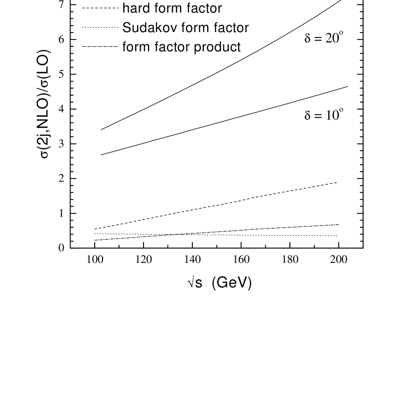
Figure 8: The total two–$b$–jet cross section (i.e. exact next–to–leading order contribution plus resummed Sudakov and non-Sudakov form factors) normalized to leading order, for the Sterman-Weinberg jet parameter choices $(\epsilon=0.1,\delta=10^{\circ}$ and $20^{\circ})$. Also shown is the separate non-Sudakov (dashed line) and Sudakov (dash-dotted line) form factor contributions, and their product (long-dashed line).

4 Conclusions

In this paper we have shown how to incorporate the exact one and two loop running coupling into the massive Sudakov as well as the hard non-Sudakov double logarithmic form factors found in $\gamma\gamma(J_{z}=0)\longrightarrow q\overline{q}$. This process is very important at a future PLC as it contains the largest background to intermediate mass Higgs production. The RG-improvement is achieved without encountering the ominous Landau-pole singularities in the hard form factor although the all orders leading and next to leading RG-solution is incorporated. The reason for this fortuitous fact is that the novel non-Sudakov form factors are “regulated” by the fermion mass, yielding an effective low energy cutoff.

The size of the effect is significant and is found to stay within the theoretical upper and lower limits for both the form factor as well as the cross section contribution. The background is enhanced significantly compared to Ref. [11] by the renormalization group effects as the effective scale is found to be roughly $9m^{2}$ for the hard form factor. The effective scale for the RG-Sudakov form factor is cutoff dependent.

In this context it is worth pointing out a major difference to the $\gamma\gamma\longrightarrow H$ signal contribution from a b-quark loop. There a function similar to the Abelian form factor of Eq. 8 occurs, as was shown in Ref. [20]. There is, however, a big difference with respect to the renormalization of the strong coupling, as in the case of $\gamma\gamma\longrightarrow H$ $\alpha_{s}$ is only renormalized at the three-loop level. The effect of the running coupling in that process is thus much smaller, but perhaps still significant in the case of a large $tan\beta$ enhancement scenario [21].

The effect of a running mass parameter is subleading as it occurs only as the arguments of logarithms. The mass term in the factorized Born amplitude is fixed by the on-shell renormalization scheme employed in the exact one loop calculation of Refs. [8, 9].

A full Monte Carlo study of both signal and background effects including investigations of optimal experimental cuts and $b$-tagging efficiencies is work in progress [22].

Acknowledgements
We would like to thank M. Wüsthoff for discussions. This work was supported in part by the EU Fourth Framework Programme ‘Training and Mobility of Researchers’, Network ‘Quantum Chromodynamics and the Deep Structure of Elementary Particles’, contract FMRX-CT98-0194 (DG 12 - MIHT).

5 Appendix

In this appendix we give explicit results for the gluon mass dependent renormalization group improved massive virtual Sudakov form factor. We also give two loop results for both the virtual as well as the sum of the virtual plus soft real contribution and show numerically that both results exponentiate.

5.1 The massive virtual RG-improved Sudakov form factor

We begin with the result for ${\cal F}^{RG}_{S_{V}}$:

$${\cal F}^{RG}_{S_{V}} = -\frac{C_{F}}{2\pi}\int^{1}_{0}\frac{d\beta_{1}}{\beta_{1}}\int^{1}_{0}\frac{d\alpha_{1}}{\alpha_{1}}\Theta(s\alpha_{1}\beta_{1}-\lambda^{2})\Theta(\alpha_{1}-\frac{m^{2}}{s}\beta_{1})\Theta(\beta_{1}-\frac{m^{2}}{s}\alpha_{1})$$ (22)

$$\times\frac{\alpha_{s}(m^{2})}{1+c\;\log\frac{s\alpha_{1}\beta_{1}}{m^{2}}}$$

$$= -\frac{C_{F}}{2\pi}\left\{\int^{\frac{\lambda}{m}}_{\frac{\lambda^{2}}{s}}\frac{d\beta_{1}}{\beta_{1}}\int^{1}_{\frac{\lambda^{2}}{s\beta_{1}}}\frac{d\alpha_{1}}{\alpha_{1}}+\int^{1}_{\frac{\lambda}{m}}\frac{d\beta_{1}}{\beta_{1}}\int^{1}_{\frac{m^{2}}{s}\beta_{1}}\frac{d\alpha_{1}}{\alpha_{1}}\right.$$

$$\left.-\int^{\frac{\lambda m}{s}}_{\frac{\lambda^{2}}{s}}\frac{d\beta_{1}}{\beta_{1}}\int^{1}_{\frac{\lambda^{2}}{s\beta_{1}}}\frac{d\alpha_{1}}{\alpha_{1}}-\int^{\frac{m^{2}}{s}}_{\frac{\lambda m}{s}}\frac{d\beta_{1}}{\beta_{1}}\int^{1}_{\frac{s}{m^{2}}\beta_{1}}\frac{d\alpha_{1}}{\alpha_{1}}\right\}\frac{\alpha_{s}(m^{2})}{1+c\;\log\frac{s\alpha_{1}\beta_{1}}{m^{2}}}$$

$$= -\frac{\alpha_{s}(m^{2})C_{F}}{2\pi}\left\{\frac{1}{c}\log\frac{s}{m^{2}}\left(\log\frac{\alpha_{s}(\lambda^{2})}{\alpha_{s}(s)}-1\right)+\frac{1}{c^{2}}\log\frac{\alpha_{s}(m^{2})}{\alpha_{s}(s)}\right\}$$

The $\lambda$-dependent terms cancel out of any physical cross section when the real Bremsstrahlung contributions are added. In order to demonstrate that the result in Eq. 22 exponentiates, we calculate the explicit two loop renormalization group improved massive virtual Sudakov corrections, now containing a different “running scale” in each loop, and find:

$${\cal F}^{{RG}_{2L}}_{S_{V}} = \frac{C^{2}_{F}}{4\pi^{2}}\int^{1}_{0}\frac{d\beta_{1}}{\beta_{1}}\int^{1}_{0}\frac{d\alpha_{1}}{\alpha_{1}}\int^{1}_{0}\frac{d\beta_{2}}{\beta_{2}}\int^{1}_{0}\frac{d\alpha_{2}}{\alpha_{2}}\frac{\alpha_{s}(m^{2})}{1+c\;\log\frac{s\alpha_{1}\beta_{1}}{m^{2}}}\frac{\alpha_{s}(m^{2})}{1+c\;\log\frac{s\alpha_{2}\beta_{2}}{m^{2}}}$$ (23)

$$\times \left\{\Theta(s\alpha_{1}\beta_{1}-\lambda^{2})\Theta(\alpha_{1}-\frac{m^{2}}{s}\beta_{1})\Theta(\beta_{1}-\frac{m^{2}}{s}\alpha_{1})\Theta(s\alpha_{2}\beta_{2}-\lambda^{2})\right.$$

$$\;\;\,\Theta(\alpha_{2}-\frac{m^{2}}{s}\beta_{2})\Theta(\beta_{2}-\frac{m^{2}}{s}\alpha_{2})\Theta(\alpha_{2}-\alpha_{1})\Theta(\beta_{2}-\beta_{1})\;\;+$$

$$\;\;\,\Theta(s\alpha_{1}\beta_{1}-\lambda^{2})\Theta(\alpha_{1}-\frac{m^{2}}{s}\beta_{1})\Theta(\beta_{1}-\frac{m^{2}}{s}\alpha_{2})\Theta(s\alpha_{2}\beta_{2}-\lambda^{2})$$

$$\;\;\,\left.\Theta(\alpha_{2}-\frac{m^{2}}{s}\beta_{1})\Theta(\beta_{2}-\frac{m^{2}}{s}\alpha_{2})\Theta(\alpha_{2}-\alpha_{1})\Theta(\beta_{1}-\beta_{2})\right\}$$

These integrals cannot be solved analytically anymore, however, numerically with the Monte Carlo generator Vegas [23] it is straightforward. Fig. 9 displays the numerical results of Eq. 23 in comparison with half of the square of the RG-improved one loop results of Eq. 22. The agreement is well within the statistical uncertainty and thus demonstrates that also the new running coupling contributions to the massive virtual Sudakov form factor exponentiates as expected. For completeness we also give the subleading terms of the pure one loop form factor which is of course also important for phenomenological applications. The complete result is thus given by:

$$\widetilde{{\cal F}}^{RG}_{S_{V}} = -\frac{\alpha_{s}(m^{2})C_{F}}{2\pi}\left\{\frac{1}{c}\log\frac{s}{m^{2}}\left(\log\frac{\alpha_{s}(\lambda^{2})}{\alpha_{s}(s)}-1\right)+\frac{1}{c^{2}}\log\frac{\alpha_{s}(m^{2})}{\alpha_{s}(s)}\right.$$ (24)

$$\left.-\frac{1}{2}\log\frac{s}{m^{2}}-\log\frac{m^{2}}{\lambda^{2}}+1-\frac{2\pi^{2}}{3}\right\}$$

Figure 9: A comparison of the second term in the exponential obtained from the renormalization group improved massive one-loop Sudakov form factor compared with the explicit two loop results. The quark mass is kept fixed at $m_{b}=4.5$ GeV and the value for the gluon mass $\lambda$ is indicated in the figure. The result in Eq. 22 clearly exponentiates.

5.2 Two loop results for the $\lambda$-independent RG-Sudakov form factor

We now give the two loop results for the physical combination ${\cal F}^{RG}_{S_{R}}+2{\cal F}^{RG}_{S_{V}}$ entering into cross sections. With the familiar Sudakov technique we find analogously to the purely virtual case:

$${\cal F}^{{RG}_{2L}}_{S_{R}}+2{\cal F}^{{RG}_{2L}}_{S_{V}} = \frac{C^{2}_{F}}{4\pi^{2}}\int^{1}_{0}\frac{d\beta_{1}}{\beta_{1}}\int^{1}_{0}\frac{d\alpha_{1}}{\alpha_{1}}\int^{1}_{0}\frac{d\beta_{2}}{\beta_{2}}\int^{1}_{0}\frac{d\alpha_{2}}{\alpha_{2}}\frac{\alpha_{s}(m^{2})}{1+c\;\log\frac{s\alpha_{1}\beta_{1}}{m^{2}}}\frac{\alpha_{s}(m^{2})}{1+c\;\log\frac{s\alpha_{2}\beta_{2}}{m^{2}}}$$ (25)

$$\times \Theta\left(\alpha_{1}+\beta_{1}-\frac{2l_{c}}{\sqrt{s}}\right)\Theta\left(\alpha_{2}+\beta_{2}-\frac{2l_{c}}{\sqrt{s}}\right)\left\{\Theta(\alpha_{1}-\frac{m^{2}}{s}\beta_{1})\right.$$

$$\Theta(\beta_{1}-\frac{m^{2}}{s}\alpha_{1})\Theta(\alpha_{2}-\alpha_{1})\Theta(\alpha_{2}-\frac{m^{2}}{s}\beta_{2})\Theta(\beta_{2}-\frac{m^{2}}{s}\alpha_{2})$$

$$\Theta(\beta_{2}-\beta_{1})+\Theta(\alpha_{1}-\frac{m^{2}}{s}\beta_{1})\Theta(\beta_{1}-\frac{m^{2}}{s}\alpha_{2})\Theta(\alpha_{2}-\alpha_{1})$$

$$\left.\Theta(\alpha_{2}-\frac{m^{2}}{s}\beta_{1})\Theta(\beta_{2}-\frac{m^{2}}{s}\alpha_{2})\Theta(\beta_{1}-\beta_{2})\right\}$$

A numerical evaluation of Eq. 25-which contains a different “running scale” for each loop-is given in Fig. 4 and compared to half the square of the one loop result in Eq. 6. It can be seen that the renormalization group improved massive Sudakov form factor exponentiates as expected.

References

- [1] J. Ellis, M.K. Gaillard, D.V. Nanopoulous, Nucl. Phys. B 106 292 (1976).
- [2] B.L. Ioffe, V.A. Khoze, Sov.J.Part.Nucl. 9 50 (1978).
- [3] I.F. Ginzburg et al., Nucl. Inst. Meth. 205 (1983) 47.
- [4] I.F. Ginzburg et al., Nucl. Inst. Meth. 219 (1984) 5.
- [5] V.I. Telnov, Nucl. Inst. Meth. A 355 (1995) 5.
- [6] G. Jikia, hep-ph/9706508 Presented at the 11th Int. Workshop on Collisions.
- [7] D.L. Borden, V.A. Khoze, J. Ohnemus and W.J. Stirling, Phys. Rev. D 50 (1994) 4499.
- [8] G. Jikia, A. Takabladze, Phys. Rev. D 54 (1996) 2030.
- [9] G. Jikia, A. Takabladze, Nucl. Inst. Meth. A 355 (1995) 81.
- [10] M. Melles, W.J. Stirling, hep-ph/9807332, to appear in Phys. Rev. D
- [11] M. Melles, W.J. Stirling, hep-ph/9810432, to appear in Eur. Phys. J.
- [12] J. Collins, Renormalisation (Cambridge University Press, Cambridge, England, 1984).
- [13] V.V. Sudakov, Sov. Phys. JETP 3 (1956) 65.
- [14] V.G. Gorshkov, V.N. Gribov, L.N. Lipatov and G.V. Frolov, Sov. J. Nucl. Phys. 6 (1967) 95.
- [15] V.S. Fadin, V.A. Khoze and A.D. Martin, Phys. Rev. D 56 (1997) 484.
- [16] S.J. Brodsky, SLAC-PUB-2447 (1979), unpublished.
- [17] Yu.L. Dokshitzer, D.I. Dyakonov, S.I. Troyan, Phys. Lett. 78 B, 290 (1978), 79B, 269 (1978) and Phys. Rept. 58, No. 5, 269 (1980).
- [18] A.B. Carter, C.H. Llewellyn Smith, Nucl. Phys. B163, 93 (1980).
- [19] I. Caprini, M. Neubert, hep-ph/9902244 and references therein.
- [20] M.I. Kotsky, O.I. Yakovlev, Phys. Lett. B418, 335 (1998).
- [21] M. Melles, hep-ph/9902428, subm. to Phys.Rev.Lett.
- [22] V.A. Khoze, M. Melles, W.J. Stirling, in progress.
- [23] P. Lepage, VEGAS, a Monte Carlo integrator, freely available, (c) 1995, Cornell University