IRB-TH-2/99

ON THE COMPLETE NEXT-TO-LEADING ORDER pQCD PREDICTION FOR THE PION FORM FACTOR

Theoretical Physics Division, Rudjer Bošković Institute, P.O. Box 1016, 10001 Zagreb, Croatia

January 1999

We comment on the results of a complete leading-twist next-to-leading order QCD analysis of the spacelike pion electromagnetic form factor at large-momentum transfer $Q$. For the asymptotic distribution amplitude, we have examined the sensitivity of the predictions to the choice of the renormalization scale. The results show that reliable perturbative predictions for the pion electromagnetic form factor can already be made at a momentum transfer $Q$ below $10$ GeV.

PACS numbers: 13.40.Gp, 12.38.Bx
Keywords: exclusive processes, perturbative QCD, next-to-leading order, pion form factor, distribution amplitudes, renormalization and factorization scales

1. Introduction

The framework for analyzing exclusive processes at large-momentum transfer within the context of perturbative QCD (pQCD) has been developed in the late seventies [1]. It was demonstrated, to all orders in perturbation theory, that exclusive amplitudes involving large-momentum transfer factorize into a convolution of a process-independent and perturbatively incalculable distribution amplitude (DA), one for each hadron involved in the amplitude, with a process-dependent and perturbatively calculable hard-scattering amplitude. In the standard hard-scattering approach (sHSA), hadron is regarded as consisting only of valence Fock states, transverse quark momenta are neglected (collinear approximation) as well as quark masses.

Although the pQCD approach of Ref. [1] undoubtedly represents an adequate and efficient tool for analyzing exclusive processes at very large momentum transfer, its applicability to these processes at experimentally accessible momentum transfer has been long debated and attracted much attention. There are several important issues regarding this subject. Let us mention first that in a moderate energy region (a few GeV) soft contributions (resulting from the competing, so-called, Feynman mechanism) can still be substantial [2], but the estimation of their size is model dependent. Further on, the self-consistency of the pQCD approach was questioned regarding the nonfactorizing end-point contributions [3]. It has been shown, that the incorporation of the Sudakov suppression in the so-called modified perturbative approach (mHSA) [4, 5] effectively eliminates soft contributions from the end-point regions and that the pQCD approach to the pion form factor begins to be self-consistent for a momentum transfer of about $Q^{2}>4$ GeV² [4]. However, in the pQCD approach to exclusive processes one still has to check its self-consistency by studying radiative corrections.

It is well known that, unlike in QED, the leading-order (LO) predictions in pQCD do not have much predictive power, and that higher-order corrections are important. In general, they have a stabilizing effect reducing the dependence of the predictions on the schemes and scales. Although the LO predictions within the sHSA (as well as, the mHSA) have been obtained for many exclusive processes, only a few processes have been analyzed at the next-to-leading order (NLO): the pion electromagnetic form factor [6, 7, 8], the pion transition form factor [7, 9] (and [10] in mHSA), and the process $\gamma\gamma\rightarrow M\overline{M}$ ($M=\pi$, $K$) [11].

In our recent work [8] we have clarified some discrepancies between previous results [6], and by including the complete closed form for the NLO evolution of the pion DA derived recently [12], we have obtained the complete NLO prediction for the pion electromagnetic form factor.

In this work we would like to give a short summary of our calculation (for details and notation see [8]) with special emphasis on the proper choice of the renormalization scale.

2. Pion electromagnetic form factor in the sHSA

In leading twist, the pion electromagnetic form factor can be written as

$$F_{\pi}(Q^{2})=\int_{0}^{1}dx\int_{0}^{1}dy\;\mathit{\Phi}^{*}(y,\mu_{F}^{2})\;T_{H}(x,y,Q^{2},\mu_{R}^{2},\mu_{F}^{2})\;\mathit{\Phi}(x,\mu_{F}^{2})\,.$$ (1)

Here $Q^{2}=-q^{2}$ is the momentum transfer in the process and is supposed to be large, $\mu_{R}$ is the renormalization scale, and $\mu_{F}$ is the factorization scale at which soft and hard physics factorize.

The hard-scattering amplitude $T_{H}(x,y,Q^{2},\mu_{R}^{2},\mu_{F}^{2})$ is the amplitude for a parallel $q_{1}\overline{q}_{2}$ pair of the total momentum $P$, with the constituents carrying the momentum fractions $x$ and $\overline{x}\,=1-x$, hit by a virtual photon $\gamma^{*}$ of momentum $q$ to end up as a parallel $q_{1}\overline{q}_{2}$ pair of momentum $P^{\prime}=P+q$, with the constituents sharing fractions $y$ and $\overline{y}\,=1-y$. It can be calculated in perturbation theory and represented as a series in the QCD running coupling constant $\alpha_{S}(\mu_{R}^{2})$:

$$T_{H}(x,y,Q^{2},\mu_{R}^{2},\mu_{F}^{2})=\alpha_{S}(\mu_{R}^{2})\,T_{H}^{(0)}(x,y,Q^{2})$$ (2)

$$\qquad\qquad\times\;\left[1+\frac{\alpha_{S}(\mu_{R}^{2})}{\pi}\,T_{H}^{(1)}(x,y,\mu_{R}^{2}/Q^{2},\mu_{F}^{2}/Q^{2})+\cdots\right]\,.$$

There are, up to the order we are calculating, 4 LO and 62 NLO Feynman diagrams that contribute to the $(q_{1}\overline{q}_{2})+\gamma^{*}\rightarrow(q_{1}\overline{q}_{2})$ amplitude. We have used the dimensional regularization method and the $\overline{MS}$ renormalization scheme in our calculation (details and results are presented in [8]).

The intuitive interpretation of the pion DA $\mathit{\Phi}(x,\mu_{R}^{2})$ ($\mathit{\Phi}^{*}(y,\mu_{R}^{2})$) is that it represents a probability amplitude for finding the valence $q_{1}\overline{q}_{2}$ Fock state in the initial (final) pion. The function ${\mathit{\Phi}}$ is intrinsically nonperturbative, but its evolution can be calculated perturbatively. It is advantageous to express the DA (further on, we use the function $\phi$ normalized to unity) in terms of the Gegenbauer polynomials

$$\phi(x)=\phi(x,\mu_{0}^{2})=\phi_{as}(x)\,\left[1+\sum_{n=2}^{\infty}{}^{\prime}B_{n}\>C_{n}^{3/2}(2x-1)\right]\,.$$ (3)

Here $\phi_{as}(x)=6x(1-x)$ is the asymptotic DA which represents the solution of the DA evolution equation for $\mu_{F}^{2}\rightarrow\infty$, while the coefficients $B_{n}$ ($n$ even) are obtained using some nonperturbative techniques at energy $\mu_{0}^{2}$. The DA is then evoluted to the energy $\mu_{F}^{2}$ and the DA evolution up to the NLO has the form

$$\phi(x,\mu_{F}^{2})=\phi^{LO}(x,\mu_{F}^{2})+\frac{\alpha_{S}(\mu_{F}^{2})}{\pi}\,\phi^{NLO}(x,\mu_{F}^{2})\,,$$ (4)

where we turn to [8] for detailed expressions.

Two most exploited choices for the pion DA (3) are $\phi_{as}(x)$ and $\phi_{CZ}(x)$, for which $B_{2}=0$ and $B_{2}=2/3$, respectively, while $B_{n}=0$ for $n>2$. Unlike $\phi_{as}(x)$, the $\phi_{CZ}(x)$ is a strongly end-point concentrated distribution and its form has been obtained using the method of QCD sum rules [13]. There is no LO evolution for $\phi_{as}(x,\mu_{F}^{2})$ and the NLO evolution is tiny. As we have shown in [8], the inclusion of the LO evolution is crucial when one tends to obtain meaningful results with the $\phi_{CZ}$ function, and even the NLO evolution is significant.

Although the numerical results for the pion electromagnetic form factor obtained by using the $\phi_{CZ}(x,\mu_{F}^{2})$ distribution are higher and closer to the existing experimental data, there are compelling theoretical results which disfavor the $\phi_{CZ}$ distribution: theoretical predictions for the pion transition form factor are in very good agreement with the data assuming that the pion distribution amplitude is close to the asymptotic one, i.e., $\phi_{as}(x,\mu_{F}^{2})$ [14]; the estimation of the size of the soft contributions to the pion electromagnetic form factor [2] indicates the asymptotic form of the pion DA, and even the self-consistency of the derivation of the $\phi_{CZ}(x,\mu_{F}^{2})$ distribution from the QCD sum rules was criticized [15]. Taking this into account, one expects that the pion DA does not differ much from the $\phi_{as}$ and in this work we comment only on the results obtained with $\phi_{as}(x,\mu_{F}^{2})$.

By inserting (2) and (4) into (1) one obtains the complete NLO pQCD expression for the pion electromagnetic form factor. Generally, one can express the NLO form factor as

$$F_{\pi}(Q^{2},\mu_{R}^{2},\mu_{F}^{2})=F_{\pi}^{(0)}(Q^{2},\mu_{R}^{2},\mu_{F}^{2})+F_{\pi}^{(1)}(Q^{2},\mu_{R}^{2},\mu_{F}^{2})\,.$$ (5)

The first term in (5) is the LO contribution, while the second term is the NLO contribution coming from the NLO correction to the hard-scattering amplitude as well as arising from the inclusion of the NLO evolution of the DA. For the results obtained using $\phi_{as}(x,\mu_{F}^{2})$ distribution, the effect of the NLO evolution of the DA is negligible ($\approx 1\%$).

3. Choosing the factorization and renormalization scales

The physical pion form factor $F_{\pi}(Q^{2})$, represented at the sufficiently high $Q^{2}$ by the factorization formula (1), is independent of the renormalization scheme and of the renormalization and factorization scales, $\mu_{R}$ and $\mu_{F}$, respectively. Truncation of the perturbative series of $F_{\pi}(Q^{2})$ at any finite order causes a residual dependence on the scheme as well as on the scales (which is already denoted in Eq. (5)). We approximate $F_{\pi}(Q^{2})$ only by two terms of the perturbative series and hope that we can minimize higher-order corrections by a suitable choice of $\mu_{R}$ and $\mu_{F}$, so that the LO term $F_{\pi}^{(0)}(Q^{2},\mu_{R}^{2},\mu_{F}^{2})$ gives a good approximation to the complete sum $F_{\pi}(Q^{2})$.

The simplest and widely used choice for the $\mu_{R}$ and $\mu_{F}$ scales is

$$\mu_{R}^{2}=\mu_{F}^{2}=Q^{2}\,,$$ (6)

the justification for the use of which is mainly pragmatic. Physically, a more appropriate choice for $\mu_{R}^{2}$ would be that corresponding to the characteristic virtualities of the particles in the parton subprocess, which is considerably lower than the overall momentum transfer $Q^{2}$ (i.e., virtuality of the probing photon). The physically motivated choices we are using are

$$\mu_{R}^{2} = \overline{x}\,\overline{y}\,Q^{2}\,,$$ (7)

$$\mu_{R}^{2} = \sqrt{(\overline{x}\,\overline{y}\,Q^{2})(\overline{y}\,Q^{2})}\,,$$ (8)

$$\mu_{R}^{2} = e^{-5/3}\overline{x}\,\overline{y}\,Q^{2}\,.$$ (9)

These correspond, respectively, to the (LO) gluon virtuality, geometrical mean of the gluon and quark virtualities (an attempt to take into account that in QCD, unlike in QED, the coupling is renormalized not only by the vector particle propagator, but also by the quark-gluon vertex and the quark-propagator, Dittes and Radyushkin [6]), and to the choice of the renormalization scale according to the Brodsky-Lepage-Mackenzie (BLM) procedure [16]. The essence of the BLM procedure is that all vacuum-polarization effects from the QCD $\beta$ function are resummed into the running coupling constant, and, as a result of the choice (9), $T_{H}^{(1)}(x,y,\mu_{R}^{2}/Q^{2},\mu_{F}^{2}/Q^{2})$ from (2) becomes $n_{f}$ (i.e. $\beta_{0}$) independent.

A glance at Eq. (1), where the coupling constant $\alpha_{S}(\mu_{R}^{2})$ appears under the integral sign, reveals that any of the choices of $\mu_{R}$ given by (7–9) leads immediately to the problem if the usual one-loop formula for the effective QCD running coupling constant is employed. To circumvent this, one can introduce a cutoff in one-loop formula with the aim of preventing the effective coupling from becoming infinite for small gluon momenta. There are number of proposals for the form of the coupling constant $\alpha_{S}(\mu_{R}^{2})$ for small $\mu_{R}^{2}$ [17, 18], but its implementation in this calculation demands the more refined treatment (see the discussion in [8]). Alternatively, one can choose $\mu_{R}^{2}$ to be an effective constant by taking $\mu_{R}^{2}=\left<\mu_{R}^{2}\right>$. Hence, in this work we have replaced the expressions (7-9) by their respective averages

$$\mu_{R}^{2} = \left<\overline{x}\,\right>^{2}Q^{2}\,,$$ (10)

$$\mu_{R}^{2} = \left<\overline{x}\,\right>^{3/2}Q^{2}\,,$$ (11)

$$\mu_{R}^{2} = e^{-5/3}\left<\overline{x}\,\right>^{2}Q^{2}\,.$$ (12)

Owing to the fact that $\phi_{as}(x,\mu_{F}^{2})$ (as well as any other pion DA) is centered around the value $x=0.5$, we take the average value of the momentum fraction to be $\left<\overline{x}\,\right>=0.5$.

We have shown in [8] that the results depend very weakly on the choice of the factorization scale $\mu_{F}$. Actually, taking $\mu_{F}^{2}$ to be an effective constant, i.e., $\mu_{F}^{2}=\left<\mu_{F}^{2}\right>$, the only $\mu_{F}^{2}$ dependence of the results obtained using $\phi_{as}(x,\mu_{F}^{2})$ distribution comes from the NLO evolution of the DA which is negligible. In the following we take $\mu_{F}^{2}=Q^{2}$.

4. Numerical results

We take that a perturbative prediction for $F_{\pi}(Q^{2})$ can be considered reliable provided the corrections to the LO prediction are reasonably small ($<30\%$) and the expansion parameter (effective QCD coupling constant) is acceptably small ($\alpha_{S}(\mu_{R}^{2})<0.3$ or $0.5$). The consistency with the experimental data is not of much use here since reliable experimental data for the pion form factor exist for $Q^{2}\leq 4$ GeV² [19] i.e., outside the region in which the perturbative treatment based on Eq. (1) is justified. It should also be mentioned that one can find controversial arguments in the literature [20] regarding the reliability of the analysis of Ref. [19]. The new data in this energy region are expected from the CEBAF experiment E-93-021.

Numerical results of our complete NLO QCD calculation for the pion form factor, $F_{\pi}(Q^{2})$, obtained using the $\phi_{as}(x,\mu_{F}^{2})$ distribution, with $\mu_{F}^{2}=Q^{2}$ and different choices for the renormalization scale $\mu_{R}^{2}$ given by (6) and (10–12), are displayed in Fig. 1a (in our calculation we take $\Lambda_{\overline{MS}}=0.2$). The ratio of the NLO to the LO contribution to $F_{\pi}(Q^{2})$, i.e., $F_{\pi}^{(1)}(Q^{2})/F_{\pi}^{(0)}(Q^{2})$, as a useful measure of the importance of the NLO corrections, is plotted as a function of $Q^{2}$ in Fig. 1b.

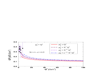
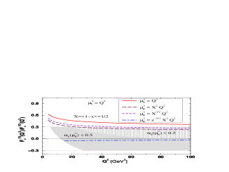
(a)	(b)

Figure 1: (a) Leading-twist NLO QCD results for $Q^{2}F_{\pi}(Q^{2})$ obtained using the $\phi_{as}(x,\mu_{F}^{2})$ distribution amplitude and the choices of $\mu_{R}^{2}$ given by Eqs. (6), (10–12), while $\mu_{F}^{2}=Q^{2}$ and $\left<\overline{x}\,\right>=0.5$. The experimental data are taken from [19]. (b) The ratio $F_{\pi}^{(1)}(Q^{2})/F_{\pi}^{(0)}(Q^{2})$ obtained using the same DA and the same choices for $\mu_{R}^{2}$ and $\mu_{F}^{2}$ scales as in Fig. 1a. The shaded area denotes the region of predictions which corresponds to $|F_{\pi}^{(1)}(Q^{2})/F_{\pi}^{(0)}(Q^{2})|<30\%$, and $\alpha_{S}(\mu_{R}^{2})\!<\!0.5$ ($\alpha_{S}(\mu_{R}^{2})\!<\!0.3$).

The solid curve in Figs. 1a and b corresponds to the often encountered choice $\mu_{R}^{2}=Q^{2}$. The total perturbative prediction $F_{\pi}(Q^{2})$ is somewhat below the trend indicated by the presently available experimental data. To make a meaningful comparison between theory and experiment, reliable experimental data are needed, as well as a reliable estimation and inclusion of the soft contributions in a moderate energy region. What alarms us is the fact that, the ratio $F_{\pi}^{(1)}(Q^{2})/F_{\pi}^{(0)}(Q^{2})$ is rather high and $F_{\pi}^{(1)}(Q^{2})/F_{\pi}^{(0)}(Q^{2})\leq 30\%$ is not reached until $Q^{2}\approx 500$ GeV². This result seems to question the applicability of the pQCD to exclusive processes. The answer to this problem lies in the previously stated inappropriateness of the choice $\mu_{R}^{2}=Q^{2}$. Namely, owing to the partitioning of the overall momentum transfer $Q^{2}$ among the particles in the parton subprocess, the essential virtualities of the particles are smaller than $Q^{2}$, so that the “physical” renormalization scale, better suited for the process of interest, is inevitably lower than $Q^{2}$.

The results displayed in Fig. 1a show that the total prediction for the pion form factor $Q^{2}F_{\pi}(Q^{2},\mu_{R}^{2},\mu_{F}^{2})$ depends weakly on the choice of $\mu_{R}^{2}$. This is a reflection of the stabilizing effect that the inclusion of the NLO corrections has on the LO predictions. By contrast, the results for the ratio $F_{\pi}^{(1)}(Q^{2},\mu_{R}^{2},\mu_{F}^{2})/F_{\pi}^{(0)}(Q^{2},\mu_{R}^{2},\mu_{F}^{2})$ are sensitive to the choice of $\mu_{R}^{2}$. From the results displayed in Fig. 1b we find that by choosing the renormalization scale related to the average virtuality of the particles in the parton subprocess or given by the BLM scale, the size of the NLO corrections is significantly reduced and reliable predictions are obtained at considerably lower values of $Q^{2}$, $Q^{2}<100$ GeV².

5. Conclusions

We conclude by stating that, regarding the size of the radiative corrections, the sHSA can be consistently applied to the calculation of the pion electromagnetic form factor. Further investigation of the scale fixing problem [21] as well as the calculation of the NLO prediction in the mHSA (the difference should be important only in the region of a few GeV) remain challenges to future work.

Acknowledgments

This work was supported by the Ministry of Science and Technology of the Republic of Croatia under Contract No. 00980102.

References

- [1] S. J. Brodsky and G. P. Lepage, Phys. Lett. B87 (1979) 359; Phys. Rev. Lett. 43(1979) 545; Phys. Rev. Lett. 43(1979) 1625 (E); G. P. Lepage and S. J. Brodsky, Phys. Rev. D 22 (1980) 2157; A. V. Efremov and A. V. Radyushkin, Theor. Mat. Phys. 42 (1980) 97; Phys. Lett. B94 (1980) 245; A. Duncan and A. H. Mueller, Phys. Lett. B90, 159 (1980); Phys. Rev. D 21 (1980) 1636.
- [2] V. Braun and I. Halperin, Phys. Lett. B328 (1994) 457; R. Jakob, P. Kroll, and M. Raulfs, J. Phys. G 22 (1996) 45; P. Kroll and M. Raulfs, Phys. Lett. B387 (1996) 848.
- [3] N. Isgur and C. H. Llewellyn Smith, Phys. Rev. Lett. 52 (1984) 1080; Phys. Lett. B217 (1989) 535; Nucl. Phys. B 317 (1989) 526; A. V. Radyushkin, Nucl. Phys. A 532 (1991) 141.
- [4] H.-N. Li and G. Sterman, Nucl. Phys. B 381 (1992) 129; D. Tung and H.-N. Li, Chin. J. Phys. 35 (1997) 651.
- [5] R. Jakob and P. Kroll, Phys. Lett. B315 (1993) 463; ibid. 319B (1993) 545(E).
- [6] R. D. Field, R. Gupta, S. Otto, and L. Chang, Nucl. Phys. B186 (1981) 429; F.-M. Dittes and A. V. Radyushkin, Sov. J. Nucl. Phys. 34 (1981) 293; M. H. Sarmadi, Ph. D. thesis, University of Pittsburgh, 1982; R. S. Khalmuradov and A. V. Radyushkin, Sov. J. Nucl. Phys. 42 (1985) 289; E. Braaten and S.-M. Tse, Phys. Rev. D 35 (1987) 2255.
- [7] E. P. Kadantseva, S. V. Mikhailov, and A. V. Radyushkin, Sov. J. Nucl. Phys. 44 (1986) 326.
- [8] B. Melić, B. Nižić, and K. Passek, hep-ph/9802204.
- [9] F. D. Aguila and M. K. Chase, Nucl. Phys. B193 (1981) 517; E. Braaten, Phys. Rev. D 28 (1983) 524.
- [10] I. V. Musatov and A. V. Radyushkin, Phys. Rev. D 56 (1997) 2713.
- [11] B. Nižić, Phys. Rev. D 35 (1987) 80.
- [12] D. Müller, Phys. Rev. D 49 (1994) 2525; Phys. Rev. D 51 (1995) 3855.
- [13] V. L. Chernyak and A. R. Zhitnitsky, Phys. Rep. 112 (1984) 173.
- [14] A. V. Radyushkin, Acta Phys. Polon. B26 (1995) 2067; S. Ong, Phys. Rev. D 52 (1995) 3111; P. Kroll and M. Raulfs, Phys. Lett. B387 (1996) 848.
- [15] A. V. Radyushkin, hep-ph/9811225.
- [16] S. J. Brodsky, G. P. Lepage, and P. B. Mackenzie, Phys. Rev. D 28 (1983) 228.
- [17] J. M. Cornwall, Phys. Rev. D 26 (1982) 1453; A. Donnachie and P. V. Landshoff, Nucl. Phys. B311 (1989) 509.
- [18] D. V.Shirkov and I. L.Solovtsov, JINR Rapid Commun. 2 [76] (1996) 5; Phys. Rev. Lett. 79 (1997) 1209; D. V. Shirkov, hep-ph/9708480.
- [19] J. Bebek et al., Phys. Rev. D 17 (1978) 1693.
- [20] C. E. Carlson and J. Milana, Phys. Rev. Lett. 65 (1990) 1717. S. Dubnička and L. Martinovič, Phys. Rev. D 39 (1989) 2079; J. Phys. G 15 (1989) 1349.
- [21] S. J. Brodsky and H. J. Lu, Phys. Rev. D 51 (1995) 3652; S. J. Brodsky, C.-R. Ji, A. Pang and D. G.Robertson, Phys. Rev. D 57 (1998) 245.