IEM-FT-189/99 IFT-UAM/CSIC-99-9 hep-ph/9903400
Strong coupling unification and extra dimensions 

Abstract

We analyze the implications of electroweak and strong coupling unification in a very general class of models extending the minimal supersymmetric standard model in $4+p$ dimensions $(p\geq 0)$. In general, electroweak precision data require the presence of large extra dimensions (low compactification scales, $M_{c}$) and/or low unification scale, $M_{U}$. In particular, the actual experimental value of the strong coupling at $M_{Z}$ imposes an upper bound on the compactification and unification scales. In four dimensional theories ($M_{c}\simeq M_{U}$) with canonical hypercharge assignment we find $M_{U}\lesssim 10^{9}$ GeV. In theories with extra dimensions ($M_{c}<M_{U}$) we find $M_{c}\lesssim 10^{7}$ GeV, for a supersymmetric spectrum at the TeV scale.

March 1999

1 Introduction

Gauge coupling unification is considered as a very suggestive hint of physics beyond the Standard Model (SM), since almost any fundamental theory describing physics at high scales predicts a sort of grand (or string) unification of gauge couplings. This idea led to rule out the SM with gauge couplings unifying in a non-supersymmetric $SU(5)$ [1], as the effective theory of electroweak and strong interactions, and to favour its minimal supersymmetric extension (MSSM) [2], on the basis of LEP and low energy precision measurements [3]. This is the most compelling ‘experimental’ indication in favour of supersymmetry at low scales (phenomenological supersymmetry). It predicts a big desert between the weak and unification scales, $M_{U}\simeq 2\times 10^{16}$ GeV, populated by the MSSM and with gauge coupling unifying at $M_{U}$ with a value $\alpha_{U}\simeq 1/24$.

However, the above picture where the MSSM unifies at $M_{U}$ is being jeopardized by the increasing precision of experimental data that demands increasing accurateness in gauge coupling unification. In particular, by imposing unification of $SU(2)\times U(1)$ gauge couplings, and the experimental input [3] ,

$$\widehat{\alpha}_{1}^{-1}(M_{Z}) = 58.98\pm 0.04$$

$$\widehat{\alpha}_{2}^{-1}(M_{Z}) = 29.57\pm 0.03$$

$$M_{Z} = 91.197\pm 0.007$$ (1.1)

it has been shown, using the two-loop renormalization group equations (RGE) [4], the $\overline{\rm MS}\rightarrow\overline{\rm DR}$ [5] conversion factors [6] and the low energy supersymmetric threshold for minimal fine tuning, that $\alpha_{3}(M_{Z})\simeq 0.13$ [7]-[9] which is $\sim$ five standard deviations away from the experimental value [3]

$$\widehat{\alpha}_{3}(M_{Z})=0.119\pm 0.002$$ (1.2)

These results correspond to the case of an $R$-parity conserving MSSM. The case of the MSSM with $R$-parity breaking couplings $\lambda$ has been recently analyzed in Ref. [10], where it is shown that the predicted value of $\alpha_{3}(M_{Z})$ is very insensitive to the values of $\lambda(M_{U})$ except possibly in the region close or beyond the non-perturbative values $\lambda^{2}(M_{U})\gtrsim 4\pi$, where the prediction can be brought to within $\sim 2\sigma$ of the observed value.

This implies that, in order to achieve successful unification, one has to rely on unknown high-energy thresholds. Without having any information about the high-energy theory this solution is unlikely to be experimentally confirmed. We will call this problem the strong unification problem.

In this paper we propose another solution to the strong unification problem based on the possible existence of large extra dimension(s). The possibility of large extra dimensions (as large as at the TeV^-1 length) [11] feeling the gauge interactions has been recently shown as very natural in a large class of string theories, in particular in type I [12]-[18] and type IIB [19] string vacua. Unlike in the perturbative heterotic string case, where one was led to identify the compactification scale, $M_{c}$, with the unification, $M_{U}$, and the string, $M_{st}$, scales $\sim 10^{18}$ GeV (creating a problem of around two orders of magnitude in the prediction of the Newton constant), in type I and IIB strings or in the non-perturbative regime of the heterotic string [20], the prediction of the string/unification scale is relaxed and can be as low as the TeV scale. This fortunate accident allows to relax the condition of a large unification scale $M_{U}$ and try to find unifying models where the strong coupling problem is resolved without any dependence on features of the underlying high-energy theory. This is the issue that will be dealt with in this paper. We will make a systematic study of models where gauge couplings unify such that the strong coupling at $M_{Z}$ lies inside the experimental range of Eq. (1.2).

In section 2 we will study 4D models that unify at any value of $M_{c}\sim M_{U}$ below the Planck scale and that solve the strong unification problem. Interestingly enough we will find that all satisfactory models unify at scales $\lesssim 10^{11}$ GeV. In section 3 we will open up the possibility of unification in $(4+p)$ dimensions provided that $M_{c}<M_{U}$. In these models the evolution of gauge couplings is logarithmic between the weak scale and $M_{c}$ and power-law between $M_{c}$ and $M_{U}$. We will find the general class of models that unify at one-loop in the same way as the MSSM. However by including two-loop corrections in the 4D theory, below $M_{c}$, we find that the experimental range (1.2) implies that $M_{U}\lesssim 10^{9}$ GeV. On the basis of the previous results we claim that gauge coupling unification prefer the presence of large extra dimension(s) feeling the gauge interactions. Finally section 4 contains our conclusions.

2 Logarithmic unification

We will start this section with some general considerations based on the one-loop unification of gauge couplings:

$$\alpha_{i}^{-1}(\Lambda)=\alpha_{i}^{-1}(\mu)-\frac{b_{i}}{2\pi}\log\frac{\Lambda}{\mu}$$ (2.1)

where $b_{i}\,(i=1,2,3)$ are the one-loop beta-functions of the model and we are (GUT) normalizing the hypercharge as: $\alpha_{1}=k_{1}g^{\prime\,2}/4\pi$, where $g^{\prime}$ is the $U(1)_{Y}$ gauge coupling and $k_{1}=5/3$ . The unification condition is then $\alpha_{1}(M_{U})=\alpha_{2}(M_{U})=\alpha_{3}(M_{U})$.

The couplings $\alpha_{1}$ and $\alpha_{2}$ meet at one-loop at the scale:

$$M_{U}^{(1)}=\mu\,e^{\,\alpha_{12}^{-1}(\mu)\,\frac{2\pi}{b_{1}-b_{2}}}$$ (2.2)

with a value

$$\alpha_{U}^{(1)\,-1}=\alpha_{1}^{-1}(\mu)-\alpha_{12}^{-1}(\mu)\ \frac{b_{1}}{b_{1}-b_{2}}=\alpha_{2}^{-1}(\mu)-\alpha_{12}^{-1}(\mu)\ \frac{b_{2}}{b_{1}-b_{2}}$$ (2.3)

where we are using the notation $\alpha_{ij}^{-1}\equiv\alpha_{i}^{-1}-\alpha_{j}^{-1}$. The one loop prediction of the strong coupling is then:

$$\alpha_{3}^{(1)\,-1}(\mu)=\alpha_{2}^{-1}(\mu)-\alpha_{12}^{-1}(\mu)\ \frac{b_{2}-b_{3}}{b_{1}-b_{2}}=\alpha_{1}^{-1}(\mu)-\alpha_{12}^{-1}(\mu)\ \frac{b_{1}-b_{3}}{b_{1}-b_{2}}\ .$$ (2.4)

Of course Eqs. (2.2), (2.3) and (2.4) should be compared with the experimental data (1) and (1.2) at the scale $\mu=M_{Z}$. From Eqs. (2.2), (2.3) and (2.4) it is obvious that given a unifying theory with beta-coefficients $b_{i}$, the new theory with beta-coefficients $\beta_{i}=b_{i}+c$, where $c$ is a constant, unifies with the same value of $M_{U}^{(1)}$ and $\alpha_{3}^{(1)}(M_{Z})$ but different value of $\alpha_{U}^{(1)}$. This happens for instance in the case where we add to the initial theory complete representations of a grand unification group which contains the gauge group of the theory. For instance in the case of the MSSM it happens when we add complete representations of $SU(5)$, or any other group containing $SU(5)$, e.g. $SO(10)$ or $E_{6}$. However this class of models, where $M_{U}^{(1)}$ is unchanged, is too restrictive and we are not interested in it. Instead we will focus on the more general class of models, characterized by the beta-coefficients $\beta_{i}$, such that only $\alpha_{3}^{(1)}(M_{Z})$ is unchanged. Using (2.4) we can see that these models must satisfy the equations:

$$\frac{b_{1}-b_{3}}{b_{1}-b_{2}}=\frac{\beta_{1}-\beta_{3}}{\beta_{1}-\beta_{2}},\quad\frac{b_{2}-b_{3}}{b_{1}-b_{2}}=\frac{\beta_{2}-\beta_{3}}{\beta_{1}-\beta_{2}}$$ (2.5)

The general solution to (2.5) is given by

$$\epsilon^{ijk}\left(b_{i}-b_{j}\right)\beta_{k}=0$$ (2.6)

It is obvious that $\beta_{i}=b_{i}$ itself belongs to the class defined by (2.6), as well as $\beta_{i}=b_{i}+c$. However, there are other models for which the prediction of $\alpha_{3}^{(1)}(M_{Z})$ is the same but with different values of $M_{U}^{(1)}$ and $\alpha_{U}^{(1)}$.

As an example, in the MSSM the one-loop beta-coefficients are given by

$$b_{i}=(33/5,1,-3)$$ (2.7)

which lead, from (2.4), to $\alpha_{3}^{(1)}(M_{Z})=0.117$, and from Eqs. (2.2) and (2.3), to $M_{U}^{(1)}=2\times 10^{16}$ GeV and $\alpha_{U}^{(1)}=1/24.3$. The class of models which predict the same value of $\alpha_{3}^{(1)}(M_{Z})$ corresponds to beta-coefficients satisfying the equation

$$5\,\beta_{1}-12\,\beta_{2}+7\,\beta_{3}=0$$ (2.8)

Then the different models satisfying Eq. (2.8) unify at different values of $M_{U}^{(1)}$ and nevertheless they lead to $\alpha_{3}^{(1)}(M_{Z})=0.117$. Some of these models will be discussed later on in this section in our general search (see Tables 1 and 2).

Two-loop corrections can lead to little differences in the final value of $\alpha_{3}(M_{Z})$ as we will see later on in this section, where we will identify several models which belong to the same class. However two loop corrections have been found to be very stable inside the same class, since there is a compensating effect for models that unify at smaller values of $M_{U}$ due to the fact that they have more extra matter, and the class (2.6) leads approximatively to the same value of $\alpha_{3}(M_{Z})$.

2.1 The MSSM

The MSSM belongs to the class (2.8) and leads, as we have already stated, to $\alpha_{3}^{(1)}(M_{Z})=0.117$. We will review the calculation of $\alpha_{3}(M_{Z})$ including two-loop corrections.

The RGE predictions for the gauge couplings in the MSSM can be written assuming unification as:

$$\alpha_{i}^{-1}(M_{Z})=\alpha_{U}^{-1}+\frac{b_{i}}{2\pi}\log\frac{M_{U}}{M_{Z}}+\frac{1}{4\pi}\sum_{j=1}^{3}\frac{b_{ij}}{b_{j}}\log\frac{\alpha_{j}(M_{U})}{\alpha_{j}(M_{Z})}+\Delta_{i}$$ (2.9)

where the two-loop beta coefficients matrix is given by:

$$b_{ij}=\left(\begin{array}[]{ccc}199/25&27/5&88/5\\ 9/5&25&24\\ 11/5&9&14\end{array}\right)$$ (2.10)

and $\Delta_{i}$ contains the $\overline{\rm MS}$ to $\overline{\rm DR}$ renormalization scheme conversion factors ($C_{2}(G_{i})/12\pi$) and the low-energy supersymmetric thresholds. Assuming for the latter that gaugino masses are degenerate at the unification scale one gets, keeping the dominant contributions to the thresholds  [7, 9]:

$$\Delta_{2} = \frac{1}{6\pi}$$

$$\Delta_{3} = \frac{1}{4\pi}+\frac{1}{28\pi}\left(28\log\frac{\alpha_{2}(M_{Z})}{\alpha_{3}(M_{Z})}+19\log\frac{M_{\rm SUSY}}{M_{Z}}\right)$$ (2.11)

where $M_{\rm SUSY}$ denotes a common supersymmetry mass.

The unification prediction from (2.9) is

$$M_{U}^{\rm MSSM} = 3.7\times 10^{16}\,{\rm GeV}$$

$$\alpha_{U}^{\rm MSSM} = 1/22.9$$

$$\alpha_{3}^{\rm MSSM}(M_{Z}) = 0.131\quad.$$ (2.12)

Therefore we see that the prediction of the MSSM is $\sim$ 5–6 standard deviations away from the experimental value (1.2) and also that the amount of all two-loop corrections in $\alpha_{3}(M_{Z})$ can be quantified to be

$$\Delta_{\rm two-loop\ }\alpha_{3}(M_{Z})\simeq 0.014$$ (2.13)

This quantity is the clue to find models solving the strong unification problem: i.e. models predicting

$$\alpha_{3}^{(1)}(M_{Z})\simeq 0.105$$ (2.14)

which will be done next.

2.2 General analysis

The first step towards the search of models which can solve the strong unification problem is to analyze the one-loop equations (2.2), (2.3) and (2.4) for a general model defined by general one-loop beta-coefficients $\beta_{i}\equiv b_{i}+\Delta b_{i}$ where $b_{i}$ are the MSSM beta-coefficients, Eq. (2.7).

Let us consider for the moment $\Delta b_{3}=0$, $\Delta b_{2}=0,1,\dots$, any value of $\Delta b_{1}$ and fix $\alpha_{3}^{(1)}(M_{Z})$ to the preferred value given in Eq. (2.14). Then we can determine $\Delta b_{1}$ as a function of $\Delta b_{2}$ which is shown in Fig. 1.

Figure 1: Plot of $\Delta b_{1}$ as a function of $\Delta b_{2}$ for $\Delta b_{3}=0$ and $\alpha_{3}^{(1)}(M_{Z})\simeq 0.105$.

The corresponding values predicted for $\alpha_{U}^{(1)}$ are plotted in Fig. 2, which shows that all these solutions are well in the perturbative regime, while the values of $M_{U}^{(1)}$ are plotted in Fig. 3.

Figure 2: Plot of $\alpha_{U}^{(1)\,-1}$ as a function of $\Delta b_{2}$ under the same conditions as in Fig. 1.

Notice first of all that the dots in Fig. 1 do not necessarily correspond to realistic models since, unlike $\Delta b_{2}$ which is being considered as a positive integer, $\Delta b_{1}$ is unconstrained in Fig. 1. So the best we can do is to try to approach the dots in Fig. 1 in particular models. Second of all, two-loop beta-coefficients do not have a direct dependence on $\Delta b_{i}$ and so two-loop corrections are model dependent and must be computed in particular models, as we will do in the following.

Figure 3: Plot of $M_{U}^{(1)}$ as a function of $\Delta b_{2}$ under the same conditions as in Fig. 1.

Before going to two-loop calculation in particular models we will discuss the case where $\Delta b_{3}>0$. To cover the whole space $(\Delta b_{1},\Delta b_{2},\Delta b_{3})$ we can proceed as follows.

• If $\Delta b_{3}\leq\min(\Delta b_{1},\Delta b_{2})$, then we can make the global shift $\Delta b_{i}\rightarrow\Delta b_{i}-\Delta b_{3}$ which shows that the corresponding model belongs to the class, in the sense of Eq. (2.6), of one of the already considered models with $\Delta b_{3}=0$. The new model will have, after two-loop corrections,

  $$\alpha_{U}^{(\Delta b_{3}>0)} > \alpha_{U}^{(\Delta b_{3}=0)}$$

  $$M_{U}^{(\Delta b_{3}>0)} < M_{U}^{(\Delta b_{3}=0)}$$

  $$\alpha_{3}^{(\Delta b_{3}>0)}(M_{Z}) \simeq \alpha_{3}^{(\Delta b_{3}=0)}(M_{Z})$$ (2.15)

  so that it will not add anything new on the analysis of $\Delta b_{3}=0$ models.

• If $\Delta b_{3}>\min(\Delta b_{1},\Delta b_{2})$ then:

  • If $\Delta b_{2}<\Delta b_{3}$ then all values $\Delta b_{1}\geq 0$ are to be considered.

  • If $\Delta b_{2}\geq\Delta b_{3}$ then only values $\Delta b_{1}<\Delta b_{3}$ should be considered.

  We have analyzed all these cases and found that, provided $M_{U}<M_{P\ell}$ , there exist no model with $\Delta b_{3}\neq 0$ and $\alpha_{3}^{(1)}(M_{Z})\simeq 0.105$.

This closes the discussion on the $\Delta b_{3}\neq 0$ case and simplifies our subsequent discussion on specific models.

2.2.1 Canonical hypercharge models

We want now to present the prediction for a very general class of models containing an arbitrary amount of extra colorless matter. Models containing color fields can be easily obtained from the latter ones by looking for cases with beta-coefficients provided by the shift $\Delta b_{i}\rightarrow\Delta b_{i}+\Delta b_{3}$ in agreement with Eq. (• ‣ 2.2) and the earlier comments. We will choose all those fields contained in $SU(5)$ representations $R_{i}$, such that $d(R_{i})\leq 24$, with arbitrary number as:

$$N_{1}(\mathbf{1},\pm 1)+N_{2}(\mathbf{2},\pm 1/2)+N_{3}(\mathbf{3},\pm 1)+n_{3}(\mathbf{3},0)$$ (2.16)

where the two labels correspond to the $SU(2)\times U(1)_{Y}$ quantum numbers, and we are summing over the $\pm$ hypercharges to cancel anomalies in a trivial way.

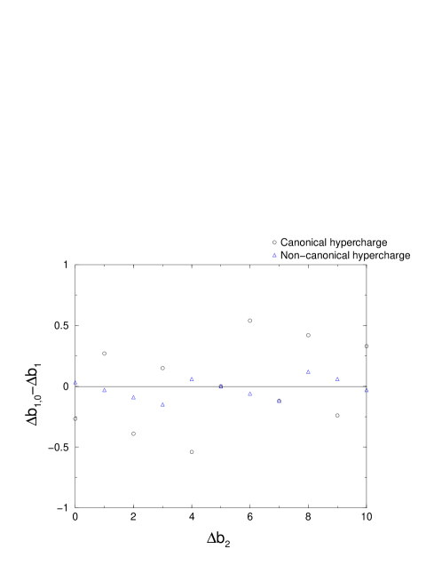
Figure 4: Nearest models, with respect to the dots in Fig. 1 $(\Delta b_{1,0},\Delta b_{2})$, which belong to the set defined by Eq. (2.16) (open circles) and Eq. (2.19) (open triangles).

The contribution of these fields to the one-loop $\Delta b_{i}$, and two-loop $\Delta b_{ij}$, beta-coefficients is given by:

$$\Delta b_{1} = \frac{3}{5}\,\left(2\,N_{1}+N_{2}+6\,N_{3}\right)$$

$$\Delta b_{2} = N_{2}+4\,N_{3}+2\,n_{3}$$ (2.17)

and

$$\Delta b_{11} = \frac{1}{25}\,\left(72\,N_{1}+9\,N_{2}+216\,N_{3}\right)$$

$$\Delta b_{12} = \frac{1}{5}\,\left(9\,N_{2}+144\,N_{3}\right)$$

$$\Delta b_{21} = \frac{1}{5}\,\left(3\,N_{2}+48\,N_{3}\right)$$

$$\Delta b_{22} = 7\,N_{2}+48\,N_{3}+24\,n_{3}$$ (2.18)

Of course, the choice of the representations in (2.16) is arbitrary and should be considered for illustrative purposes. However, higher dimensional representations would not alter the general analysis since they contribute to $\Delta b_{2}$ with higher values, and their net effect could always be replaced by a set of lower dimensional representations. In particular the colorless representations with integer electric charge can be written in terms of $SU(2)\times U(1)$ quantum numbers as: $(\mathbf{2J+1},\pm Y)$ with $J=0,\,1/2,\,1,\,3/2,\,2,\dots$ and $Y$ an integer (half-integer) for $J$ integer (half-integer). Their contribution to the beta-coefficients is increasing with the dimension as $\Delta b_{2}(\mathbf{1},\mathbf{2},\mathbf{3},\mathbf{4},\mathbf{5},\dots)=(0,1/2,2,5,10,\dots)$.

The nearest models in the $(\Delta b_{1},\Delta b_{2})$-plane, with respect to the dots in Fig. 1 with ordinate denoted by $\Delta b_{1,0}$, which belong to the set of models defined in Eq. (2.16) are shown in Fig. 4 (see open circles) for values of $\Delta b_{2}\leq 10$. The particular values of the parameters $N_{1},N_{2},N_{3},n_{3}$ for the corresponding models are exhibited in Table 1 where the predictions of $\alpha_{3}^{(1)}(M_{Z})$ and $\alpha_{3}(M_{Z})$ (two-loop calculation) are also shown. When two models are shown (which is the case for $\Delta b_{2}\leq 4$) the nearest model corresponds to that on the left column, and the next-to-nearest model to that on the right column. We can see that models with $\Delta b_{1}>\Delta b_{1,0}$, which are located in the lower half-plane of Fig. 4 ($\Delta b_{1}<\Delta b_{1,0}$, located in the upper half-plane of Fig. 4) have $\alpha_{3}^{(1)}(M_{Z})>0.105$ ($\alpha_{3}^{(1)}(M_{Z})<0.105$) and the two-loop calculation gives values of $\alpha_{3}(M_{Z})$ which are larger (smaller) than the experimental value (1.2). In fact for the values of $\Delta b_{2}$ for which two models are presented, one of them predicts a value of $\alpha_{3}(M_{Z})$ smaller and the other larger than the experimental value (1.2).

Two-loop corrections are computed using the beta-coefficients (2.2.1). Extra matter is considered at the TeV scale and we have assumed absolute degeneracy in the supermultiplets and no threshold effect.

$\Delta b_{1}$	$\Delta b_{2}$	$N_{1}$	$N_{2}$	$N_{3}$	$n_{3}$	$\alpha_{3}^{(1)}(M_{Z})$	$\alpha_{3}(M_{Z})$
0, 6/5	0	0,1	0,0	0,0	0,0	0.117, 0.083	0.131, 0.087
3, 9/5	1	2,1	1,1	0,0	0,0	0.099, 0.148	0.106, 0.181
24/5, 6	2	4,5	0,0	0,0	1,1	0.117, 0.091	0.134, 0.097
39/5, 33/5	3	6,5	1,1	0,0	1,1	0.103, 0.137	0.114, 0.168
48/5, 54/5	4	5,6	0,0	1,1	0,0	0.117, 0.096	0.135, 0.104
63/5	5	7	1	1	0	0.106	0.118
78/5	6	10	0	1	1	0.099	0.110
87/5	7	11	1	1	1	0.108	0.122
102/5	8	1	0	2	0	0.101	0.113
111/5	9	12	1	2	0	0.109	0.124
126/5	10	15	0	2	1	0.103	0.117

Table 1: Values of $\alpha_{3}(M_{Z})$ for models with canonical hypercharge.

From Table 1 we see that there are models which belong to the same equivalence class, in the sense of Eq. (2.6). For instance, models on the left column with $\Delta b_{2}=0,2,4$ belong to the MSSM equivalence class and could have been found just by exploring the corresponding equation (2.8). We can also see that in order to corner values of $\alpha_{3}(M_{Z})$ inside the experimental range (1.2) we have to go to $\Delta b_{2}=5$ $(N_{1}=7,\,N_{2}=N_{3}=1)$ and this model predicts values of the unification scale and gauge coupling given by: $M_{U}=5\times 10^{8}$ GeV and $\alpha_{U}=1/15.4$.

Let us finally stress that all presented models have $\Delta b_{3}=0$. Following our general comments at the beginning of this section, models with $\Delta b_{3}>0$ can be found, which belong to the same class as models with $\Delta b_{3}=0$, and with unification scales and couplings as given by Eq. (• ‣ 2.2). In particular they have smaller unification scale than $\Delta b_{3}=0$ models. Therefore the requirement of gauge coupling unification has led us to a general upper bound on the unification scale as: $M_{U}\lesssim 5\times 10^{8}$ GeV.

2.2.2 Non-canonical hypercharge models

Of course with non-canonical hypercharge assignment there is much more freedom in the choice of extra matter. For the sake of illustration we will consider a particular $SU(4)_{c}\times SU(2)_{L}\times SU(2)_{R}$ string model [21] that breaks to $SU(3)_{c}\times SU(2)_{L}\times U(1)_{Y}$ at the scale $M_{U}$. If the latter scale coincides with the string scale $M_{st}$ the gauge couplings should unify at $M_{U}$ and we can constrain its value from the unification condition, similarly to what we have done in the previous section for general models with canonical hypercharge assignment. The $SU(3)_{c}\times SU(2)_{L}\times U(1)_{Y}$ quantum numbers of the extra matter is:

$$N_{2}\,(\mathbf{1},\mathbf{2},\pm 1/2)+N^{\prime}\,(\mathbf{1},\mathbf{1},\pm 1/2)+2\,N_{L}\,(\mathbf{1},\mathbf{2},0)$$ (2.19)

$$+ N_{3}\,(\mathbf{3},\mathbf{1},\pm 1/3)+N^{\prime}_{3}\,(\mathbf{3},\mathbf{1},\pm 1/6)+N_{31}\,(\mathbf{3},\mathbf{1},\pm 2/3)$$

where we assume we are summing over $\pm$ non-zero hypercharges so the corresponding labels count the number of pairs. On the other hand we can see there can be colorless matter with fractional electric charge, which is a general feature in many string models.

The field content of (2.19) contribute to the one-loop and two-loop beta functions, $\Delta b_{i}$ and $\Delta b_{ij}$, respectively. However, following the general analysis at the beginning of this section, in the search of models and their unification scales $M_{U}$, it is enough to consider the cases where $\Delta b_{3}=0$ and $\Delta b_{3i}=\Delta b_{i3}=0$, which amounts to take into account only colorless states, those on the first row of Eq. (2.19). Their contribution to the beta-coefficients can be written as:

$$\Delta b_{1} = \frac{3}{5}\,\left(N_{2}+\frac{N^{\prime}}{2}\right)$$

$$\Delta b_{2} = N_{2}+N_{L}$$ (2.20)

and

$$\Delta b_{11} = \frac{1}{25}\,\left(72\,N_{1}+\frac{9}{2}\,N^{\prime}\right)$$

$$\Delta b_{12} = \frac{9}{10}\,N_{2}$$

$$\Delta b_{21} = \frac{3}{5}\,N_{2}$$

$$\Delta b_{22} = 7\,N_{2}+7\,N_{L}$$ (2.21)

The nearest models in the $(\Delta b_{1},\Delta b_{2})$-plane, with respect to the dots in Fig. 1, which belong to the set of models defined in Eq. (2.19) are shown in Fig. 4 (see open triangles) for values of $\Delta b_{2}\leq 10$. The particular value of the parameters $N_{2},N^{\prime},N_{L}$ for the corresponding models is exhibited in Table 2 where the predictions of $\alpha_{3}^{(1)}(M_{Z})$ and $\alpha_{3}(M_{Z})$ (two-loop calculation) are also shown. We can see (as in the case of canonical hypercharge) that models with $\Delta b_{1}>\Delta b_{1,0}$, which are located in the lower half-plane of Fig. 4 ($\Delta b_{1}<\Delta b_{1,0}$, located in the upper half-plane of Fig. 4) have $\alpha_{3}^{(1)}(M_{Z})>0.105$ ($\alpha_{3}^{(1)}(M_{Z})<0.105$) and the two-loop calculation gives values of $\alpha_{3}(M_{Z})$ which are larger (smaller) than the experimental value (1.2). Two-loop corrections are computed using the beta-coefficients (2.2.2). Again extra matter is considered at the TeV scale and we have assumed absolute degeneracy in the supermultiplets and no threshold effect.

$\Delta b_{1}$	$\Delta b_{2}$	$N_{2}$	$N_{L}$	$N^{\prime}$	$\alpha_{3}^{(1)}(M_{Z})$	$\alpha_{3}(M_{Z})$
3/10	0	0	0	1	0.105	0.114
27/10	1	1	0	7	0.107	0.116
51/10	2	1	1	15	0.108	0.119
36/5	3	2	1	20	0.117	0.131
51/5	4	2	2	30	0.105	0.114
63/5	5	4	1	34	0.106	0.116
15	6	4	2	41	0.107	0.117
87/5	7	5	2	48	0.108	0.118
201/10	8	6	2	55	0.105	0.115
45/2	9	6	3	63	0.105	0.116
249/10	10	7	3	69	0.106	0.117

Table 2: Values of $\alpha_{3}(M_{Z})$ for models with non-canonical hypercharge.

We can see that the prediction of $\alpha_{3}(M_{Z})$ for the models from Table 2 is much closer to the experimental range (1.2) than for those with canonical hypercharge assignment from Table 1. In particular the model with $\Delta b_{2}=0$ predicts a value of $\alpha_{3}(M_{Z})$ which is 2.5$\sigma$, and the model with $\Delta b_{2}=1$ is only 1.5$\sigma$. However the first model where $\alpha_{3}(M_{Z})$ is inside the experimental range corresponds to $\Delta b_{2}=2$, which unifies at $M_{U}=5\times 10^{11}$ GeV with $\alpha_{U}=1/18.5$.

The class of models defined by Eq. (2.19) has been recently analyzed by the authors of Ref. [22]. The values for the matter content $(N_{2},N^{\prime},N_{L})$ they obtain for acceptable models do not coincide with those appearing in Table 2. The reason is that in Ref. [22] only the one-loop RGE analysis has been performed while we are including two-loop corrections (and MSSM weak scale threshold effects), which are sizable as stated in Eq. (2.13).

To conclude, in the class of string models defined by the extra particle content (2.19), strong coupling unification implies that $M_{U}\lesssim 5\times 10^{11}$ GeV.

3 Power-law unification

Another possibility, which has been recently stressed by Dienes, Dudas and Gherghetta [23], is based on a $4+p$ dimensional theory with a (common) compactification radius for the extra $p$ dimensions $M_{c}^{-1}$, with $M_{c}\ll M_{U}$, which leads to much lower values of the unification scale $M_{U}$. Under these conditions, the $p$ extra dimensions open up at the scale $M_{c}$ and the gauge coupling renormalization receive the contribution of the towers of Kaluza-Klein (KK) excitations which make them to run with a power-low behaviour [24]. Under certain circumstances, that we will analyze in full generality next, the gauge couplings unify shortly after $M_{c}$. In the case where there is a hierarchy among the radii of $p$ dimensions, the theory for scales greater than $1/R_{5}$ behaves as five dimensional, evolution of the gauge couplings is accelerated and they may unify at a scale $\lesssim 1/R_{6}$. For this reason we will consider, for the computational sake, the case of a 5D theory, with $M_{c}$ the inverse radius of the fifth dimension, although our results are completely general.

We will consider the 5D theory compactified on the fifth dimension orbifold $S^{1}/\mathbb{Z}_{2}$ [25, 26]. Half of the KK modes is projected away by the action of $\mathbb{Z}_{2}$, which means that for zero-modes the theory has $N=1$ supersymmetry, while non-zero modes keep their $N=2$ nature and utilize the odd-modes to reconstruct entire KK-towers, whose number is therefore divided by two. A full explanation of this kind of models can be found in Refs. [26]. The MSSM is made up of zero-modes of fields living in the 5D bulk and fields that can live in the 4D boundary, at localized points of the bulk. (Fixed points in the language of the heterotic string.) The fields that live on the 4D boundary are arranged in $N=1$ supermultiplets and those living in the bulk in $N=2$ supermultiplets.

Vector fields in the bulk are in $N=2$ vector supermultiplets. For non-zero (massive) KK-modes they contain a massive vector field, a real scalar and a Dirac fermion. For zero (massless) KK-modes, only the $N=1$ vector supermultiplet survive the $\mathbb{Z}_{2}$ projection. Chiral fields in the bulk belong to $N=2$ hypermultiplets. They contain two complex scalars and a Dirac fermion. For the zero-modes only one complex scalar and a particular chiral projection of the Dirac fermion survive after $\mathbb{Z}_{2}$ projection. This is the case of the Higgs and matter sector $(H_{1},H_{2},Q,U,D,L,E)$. Whenever they live in the bulk, they should constitute an independent hypermultiplet which, after $\mathbb{Z}_{2}$ projection leads to the supermultiplet structure of the MSSM .

The generic scenario is the following. We have a 4D model valid up to the compactification scale $M_{c}$. Its particle content consists on (half of) the zero-modes of fields living in the bulk plus fields living on the boundary. The 4D fields are arranged in $N=1$ supermultiplets and the gauge coupling evolution is logarithmic. The 4D model can be any of the models previously considered. Given the particular model, characterized by beta-coefficients $b_{i}$ and a particular value of $\alpha_{3}^{(1)}(M_{Z})$, from the 4D formula (2.4), when the extra dimension opens up at the scale $M_{c}$ the states that contribute to the gauge coupling renormalization for scales beyond $M_{c}$ are:

1. Fields living on the boundary, that contribute logarithmically to the renormalization of the gauge couplings.

2. Fields living in the bulk which constitute towers of $N=2$ supermultiplets, with beta functions $\widetilde{b}_{i}$, that contribute with a power-law to the gauge coupling renormalization.

The one-loop evolution is then given by:

$$\alpha^{-1}_{i}(\Lambda)=\alpha^{-1}_{i}(\mu)-\frac{b_{i}}{2\pi}\log\frac{\Lambda}{\mu}-\frac{\widetilde{b}_{i}}{2\pi}\left(\frac{\Lambda}{M_{c}}-1-\log\frac{\Lambda}{M_{c}}\right)$$ (3.1)

From Eq. (3.1) we can deduce analytical equations for $M_{U}^{(1)}$, $\alpha_{U}^{(1)}$ and $\alpha_{3}^{(1)}(M_{c})$ by imposing unification and neglecting the logarithmic running between $M_{c}$ and $M_{U}$. We obtain equations similar to those obtained for the logarithmic running in 4D (2.2), (2.3) and (2.4):

$$M_{U}^{(1)}=\alpha_{12}^{-1}(M_{c})\,\frac{2\pi}{\widetilde{b}_{1}-\widetilde{b}_{2}}\ M_{c}=\frac{b_{1}-b_{2}}{\widetilde{b}_{1}-\widetilde{b}_{2}}\ M_{c}\ \log\frac{M_{U}^{(1)\,{\rm 4D}}}{M_{c}}$$ (3.2)

where $M_{U}^{(1)\,{\rm 4D}}$ is the 4D prediction of $M_{U}$ as given by (2.2),

$$\alpha_{U}^{(1)\,-1}=\alpha_{1}^{-1}(M_{c})-\alpha_{12}^{-1}(M_{c})\ \frac{\widetilde{b}_{1}}{\widetilde{b}_{1}-\widetilde{b}_{2}}=\alpha_{2}^{-1}(M_{c})-\alpha_{12}^{-1}(M_{c})\ \frac{\widetilde{b}_{2}}{\widetilde{b}_{1}-\widetilde{b}_{2}}$$ (3.3)

$$\alpha_{3}^{(1)\,-1}(M_{c})=\alpha_{2}^{-1}(M_{c})-\alpha_{12}^{-1}(M_{c})\ \frac{\widetilde{b}_{2}-\widetilde{b}_{3}}{\widetilde{b}_{1}-\widetilde{b}_{2}}=\alpha_{1}^{-1}(M_{c})-\alpha_{12}^{-1}(M_{c})\ \frac{\widetilde{b}_{1}-\widetilde{b}_{3}}{\widetilde{b}_{1}-\widetilde{b}_{2}}$$ (3.4)

We can match the prediction of the theory for $\alpha_{3}^{(1)}(M_{c})$ running with a power law from $M_{U}$, as given by (3.4), with that of the 4D theory running logarithmically from $M_{Z}$, as given by (2.4) with $\mu=M_{c}$. Then the 5D theory predicts at one-loop the same value of $\alpha_{3}^{(1)}(M_{Z})$ as the 4D theory provided that the conditions

$$\frac{b_{1}-b_{3}}{b_{1}-b_{2}}=\frac{\widetilde{b}_{1}-\widetilde{b}_{3}}{\widetilde{b}_{1}-\widetilde{b}_{2}},\quad\frac{b_{2}-b_{3}}{b_{1}-b_{2}}=\frac{\widetilde{b}_{2}-\widetilde{b}_{3}}{\widetilde{b}_{1}-\widetilde{b}_{2}}$$ (3.5)

hold, whose general solution is:

$$\epsilon^{ijk}\left(b_{i}-b_{j}\right)\,\widetilde{b}_{k}=0$$ (3.6)

Notice that the equation (3.6) is similar to the class condition for 4D models (2.6), which shows that the strong coupling unification condition at one-loop is independent on the dimensionality.

We will now consider the case of the MSSM for two reasons. On the one hand simplicity, since our aim is to prove that the MSSM can solve the strong unification problem in the presence of large extra dimensions, and find an upper bound on the value of the compactification and unification scales. The second reason is that models considered in section 2 would lead to a lower value of the unification scale than that provided by the MSSM and the study of those models would not add anything new concerning the former upper bound.

In the case of the MSSM the unification condition (3.6) reads as:

$$5\,\widetilde{b}_{1}-12\,\widetilde{b}_{2}+7\,\widetilde{b}_{3}=0\,$$ (3.7)

where now $\widetilde{b}_{i}$ are the $N=2$ beta-coefficients, given by:

$$\widetilde{b}_{i}=-2\left(C_{2}(G_{i})-T(R)\right)$$ (3.8)

and $R$ are the representations which the hypermultiplets belong to. Assuming a general $N=2$ superfield content, with $N_{X}$ hypermultiplets $X$ $(X=Q,U,D,L,E,H_{1},H_{2})$ and $\delta_{G}$ vector multiplets $(G=SU(3),SU(2),U(1))$ living in the bulk $(\delta_{G}=0,1)$, the condition (3.7) can be written as:

$$2\,N_{E}+5\,N_{U}-7\,N_{Q}+3\,\left(N_{D}-N_{L}\right)=14\,\delta_{SU(3)}-16\,\delta_{SU(2)}+3\,\left(N_{H_{1}}+N_{H_{2}}\right)$$ (3.9)

However, not all values of the parameters are attainable in Eq. (3.9), since we must require that hypermultiplets in the bulk experience gauge interactions in the $N=2$ theory. Therefore, on general grounds we can split Eq. (3.9) into three different possible cases, depending on the possible values of $\delta_{G_{i}}$.

1. The case where the $SU(3)\times SU(2)\times U(1)$ gauge bosons are in the bulk. In this case $\delta_{SU(3)}=\delta_{SU(2)}=1$ and Eq. (3.9) reads as

   $$2\,N_{E}+5\,N_{U}-7\,N_{Q}+3\,\left(N_{D}-N_{L}\right)-3\,\left(N_{H_{1}}+N_{H_{2}}\right)+2=0$$ (3.10)

2. The case where only the $SU(3)\times U(1)$ gauge bosons are in the bulk. In this case $\delta_{SU(3)}=1,\,\delta_{SU(2)}=0$, $N_{Q}=N_{L}=N_{H_{i}}=0$ (no $SU(2)$-doublets in the bulk), and Eq. (3.9) reads as

   $$2\,N_{E}+5\,N_{U}+3\,N_{D}=14$$ (3.11)

3. The case where only the $SU(2)\times U(1)$ gauge bosons are in the bulk. In this case $\delta_{SU(3)}=0,\,\delta_{SU(2)}=1$, $N_{U}=N_{Q}=N_{D}=0$ (no $SU(3)$-triplets in the bulk), and Eq. (3.9) reads as

   $$2\,N_{E}+16=3\,\left(N_{L}+N_{H_{1}}+N_{H_{2}}\right)$$ (3.12)

Notice that the $U(1)$ gauge multiplet should be situated in the bulk, if hypermultiplets with hypercharge live in the bulk, since they should experience the corresponding gauge interactions. In the particular case of no hypermultiplets in the bulk, the $U(1)$ gauge multiplet can be either in the bulk or on the boundary. This leads to the trivial solution to Eq. (3.9) where all matter, except the $U(1)$ gauge boson, is at the boundary. In this case the beta-coefficients $\widetilde{b}_{i}=0$, the evolution beyond $M_{c}$ is logarithmic and the unification is like in the 4D MSSM, Eqs. (2.1). Still the $U(1)$ in the bulk can be used to break supersymmetry by the Scherk-Schwarz mechanism by giving a mass to the $\widetilde{B}$ gaugino, with the subsequent propagation of supersymmetry breaking to the boundary by radiative corrections [26].

Any matter content in the bulk consistent with Eq. (3.9) will then provide a model where the one-loop prediction of $\alpha_{3}(M_{Z})$ is as in the MSSM but with $M_{U}$ and $\alpha_{U}$ differently determined, Eqs. (3.2) and (3.3). Particular cases satisfying Eqs. (3.10)-(3.12) have recently been proposed in the literature:

• The case where the gauge and Higgs sector, along with two $E$ hypermultiplets, is in the bulk, $(\delta_{SU(3)}=\delta_{SU(2)}=N_{H_{1}}=N_{H_{2}}=1,N_{E}=2)$, has been discussed by Kakushadze [28]. It belongs to case 1 before and satisfies Eq. (3.10). Other possibilities are obvious from Eq. (3.10), apart from those corresponding to complete $SU(5)$ representations: $N_{E}=N_{U}=N_{Q}$ and/or $N_{D}=N_{L}$.

• The case $\delta_{SU(3)}=1,\,\delta_{SU(2)}=0$, $N_{U}=N_{D}=1$, $N_{E}=3$ has been discussed recently by Carone [27]. It satisfies Eq. (3.11) and belongs to case 2 before. Other trivial possibilities are, e.g.: a) $N_{U}=N_{E}=2$, the other $N_{i}$ equal to zero; b) $N_{D}=2$, $N_{E}=4$, the other $N_{i}$ equal to zero.

• The case $\delta_{SU(3)}=0,\,\delta_{SU(2)}=1$, $N_{E}=N_{H_{1}}=1$, $N_{L}=5$ has also been discussed in Ref. [27]. It satisfies Eq. (3.12) and belongs to case 3 before. There are of course other trivial possibilities satisfying Eq. (3.12) as, e.g.: a) $N_{E}=N_{H_{i}}=1$, $N_{L}=4$; b) $N_{E}=4$, $N_{H_{i}}=1$, $N_{L}=6$.

It is clear that a great variety of models satisfying Eq. (3.9) can be discussed and proposed, leading to very similar values of the unification scale and coupling at the one-loop level. In all cases the hypermultiplets in (3.9) can be considered either as extra matter (with respect to the MSSM) which decouples at $M_{c}$ , or as part of the MSSM .

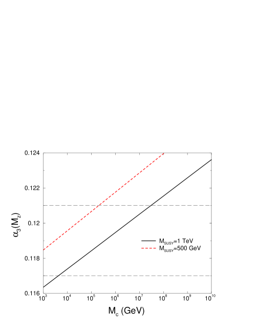
Figure 5: Value of $\alpha_{3}(M_{Z})$ versus $M_{c}$. The two horizontal lines represent the experimental 1$\sigma$ band.

To make a more accurate prediction for this class of models we will include, as in Ref. [29], two-loop effects between the weak scale and $M_{c}$, the $\overline{\rm MS}$ to $\overline{\rm DR}$ conversion factors and the MSSM supersymmetric threshold effects as in section 2. Then the RGE predictions for the gauge couplings can be written as:

$$\alpha_{i}^{-1}(M_{Z}) = \alpha_{U}^{-1}+\frac{b_{i}}{2\pi}\log\frac{M_{U}}{M_{Z}}+\frac{1}{4\pi}\sum_{j=1}^{3}\frac{b_{ij}}{b_{j}}\log\frac{\alpha_{j}(M_{U})}{\alpha_{j}(M_{Z})}+\Delta_{i}$$ (3.13)

$$+ \frac{\widetilde{b}_{i}}{2\pi}\left(\frac{M_{U}}{M_{c}}-1-\log\frac{M_{U}}{M_{c}}\right)$$

The numerical results are shown in Fig. 5 where the prediction of $\alpha_{3}(M_{Z})$ is plotted versus $M_{c}$ for two particular values of the common supersymmetry breaking mass $M_{\rm SUSY}$ (500 GeV and 1 TeV). Then from the experimental band for $\alpha_{3}(M_{Z})$ we obtain an upper bound for $M_{c}$ as $M_{c}\lesssim 2\times 10^{7}$ GeV for $M_{\rm SUSY}$=1 TeV and $M_{c}\lesssim 1.5\times 10^{5}$ GeV for $M_{\rm SUSY}$=500 GeV. The corresponding values of $M_{U}$ can be obtained easily from (3.2). There is a mild model dependence from the term $b_{12}/\widetilde{b}_{12}$, although this term is usually $\mathcal{O}(1)$. To fix the ideas, and as an illustration, in the model with $(\delta_{SU(3)}=\delta_{SU(2)}=N_{H_{1}}=N_{H_{2}}=1,N_{E}=2)$ of Ref. [28], $(b_{1}-b_{2})/(\widetilde{b}_{1}-\widetilde{b}_{2})=1$, and $M_{U}\lesssim 4.4\times 10^{8}$ GeV for $M_{\rm SUSY}$=1 TeV, $M_{U}\lesssim 4\times 10^{6}$ GeV for $M_{\rm SUSY}$=500 GeV.

A word of caution has to be said about this result. In our RGE for the evolution of the gauge couplings from $M_{Z}$ to $M_{U}$ we have considered two-loop effects below $M_{c}$ as well as supersymmetric threshold effects at the weak scale. However no two-loop effect beyond $M_{c}$ has been considered. This issue has been studied in Ref. [28] where, using the fact that the gauge coupling is not renormalized beyond one-loop in the $N=2$ theory , it was estimated that the ratio of two-to-one loop renormalization of the inverse gauge coupling goes as:

$$\Delta^{(2)}\,\alpha_{i}^{-1}=\mathcal{O}\left(\frac{M_{c}}{\Lambda}\right)\Delta^{(1)}\,\alpha_{i}^{-1}$$

where $\Lambda$ is identified here as the cutoff of the theory. This means that perturbation theory seems to be trustable but nevertheless the (accelerated) unification predictions are not guaranteed to survive to higher loop corrections. A preliminary calculation of two-loop corrections for scales beyond $M_{c}$ has shown that the leading corrections, in particular those with bulk and boundary fields mixed in the diagram, are very model dependent. In particular they depend on the distribution of matter in bulk hypermultiplets and boundary chiral multiplets. A detailed calculation of these two-loop corrections is outside the scope of this paper and will be postponed for future work.

Finally, let us stress that models with extra dimensions at the TeV scale are favoured by gauge coupling ‘accelerated’ unification. In this case the extra dimensions could be used to trigger supersymmetry breaking by the Scherk-Schwarz  mechanism [26], and lead to observable effects in high-energy colliders by the production of Kaluza-Klein excitation of the MSSM particles [11, 32]. In particular, if we fix in Fig. 5 $M_{c}=1$ TeV one obtains $\alpha_{3}(M_{Z})=0.1165$ for $M_{\rm SUSY}=1$ TeV and $\alpha_{3}(M_{Z})=0.1185$ for $M_{\rm SUSY}=0.5$ TeV, in rather good agreement with precision data.

4 Conclusions

In this paper we have analyzed the unification of $SU(3)\times SU(2)\times U(1)$ gauge couplings in supersymmetric extensions of the Standard Model, using the gauge couplings determination at $M_{Z}$ deduced from LEP and low energy precision measurements. We have considered two very general unification scenarios:

Logarithmic unification

This is the case where unification is achieved in an $N=1$ four-dimensional theory and, therefore, the evolution of gauge couplings is logarithmic. We impose unification of general supersymmetric models and perturbativity, and obtain the unification scale $M_{U}$, that we assume to be of the order of magnitude of the compactification scale where new dimensions open up, $M_{c}$.

Power-law unification

In this case the extra dimensions open up at scales $M_{c}$ much lower than the unification scale and, beyond $M_{c}$, gauge couplings run, as functions of the energy, with a power-law behaviour. Unification happens in an ‘accelerated’ way during the last stages of their evolution. The theory below $M_{c}$ is $N=1$ supersymmetric and beyond $M_{c}$ the Kaluza-Klein states form multiplets of $N=2$ supersymmetry. We consider, below $M_{c}$ the MSSM, and beyond it a general class of $N=2$ models that provide the same one-loop strong coupling at $M_{Z}$ as the MSSM. The experimental range for the gauge couplings provide a corresponding band in $M_{c}$, and in $M_{U}$, with an upper bound, which implies in general large extra dimensions.

In the case of logarithmic unification we have examined the general set of models with canonical hypercharge (such that colorless extra fields have integer electric charge), and also a class of unifying string models with fractional electric charge for colorless states, with unification gauge group $SU(4)\times SU(2)\times SU(2)$. The experimental upper bound on $\alpha_{3}(M_{Z})$ translates into an upper bound on the unification scale which is $\sim 10^{9}$ GeV for the canonical hypercharge models and $\sim 10^{12}$ GeV for string models.

In the case of power-law unification we have examined the general class of models which coincide with the MSSM in 4D, below the compactification scale $M_{c}$, and that unify in $(4+p)$ dimensions with the same one-loop value of $\alpha_{3}(M_{Z})$ as the MSSM. Inclusion of two-loop corrections below $M_{c}$ provides upper bounds on $M_{c}$ and $M_{U}$ ($\sim 10^{7}$ GeV and $\sim 10^{9}$ GeV, respectively) from the unification constrains. However, before drawing definite predictions in this case higher loop corrections from Kaluza-Klein excitations should be precisely computed.

In either case, logarithmic or power-law unification, it is possible that the size of the required extra dimension is $\sim$ TeV^-1. This fact makes it possible that:

• The extra dimension have observable effects in high-energy colliders. These effects can either put lower bounds on the mass of the corresponding KK-excitations, in the case of negative searches, or enable their experimental direct discovery [11, 32].

• The extra dimensions be used, as a useful mechanism to break supersymmetry by the Scherk-Schwarz compactification, creating a mass splitting between members of the same supermultiplet. The main features of this mechanism have been extensively studied [26].

All along this paper we have used GUT-like unification condition, i.e. $\alpha_{3}(M_{U})=\alpha_{2}(M_{U})=k_{1}\alpha_{Y}(M_{U})$ where $k_{1}=5/3$. This is the case in grand unification and many string theories. However in some string constructions other values of $k_{1}$ may appear that can help to solve in a different fashion the strong coupling problem. We wish to mention here this possibility, which has been already stressed in the literature. Just to give an illustrative example, in the case of $k_{1}=7/4$ the predictions of the MSSM including the same corrections as those considered in section 2 are:

$$M_{U} = 9.7\times 10^{15}\,\mathrm{GeV}$$

$$\alpha_{U} = 1/23.2$$

$$\alpha_{3}(M_{Z}) = 0.116$$ (4.1)

where $\alpha_{3}(M_{Z})$ is now in rough agreement with the experimental data.

To conclude we have proved that the unification of gauge couplings, as deduced from the electroweak precision data, requires in a general class of models the presence of large extra dimensions (as large as $\mathrm{TeV}^{-1}$) and/or low unification scale.

References

- [1] H. Georgi and S.L. Glashow, Phys. Rev. Lett. 32 (1974) 275; H. Georgi, H.R. Quinn and S. Weinberg, Phys. Rev. Lett. 33 (1974) 451.
- [2] J. Ellis, S. Kelley and D.V. Nanopoulos, Phys. Lett. B249 (1990) 441; U. Amaldi, W. de Boer and H. Furstenau, Phys. Lett. B260 (1991) 447.
- [3] Reviews of Particle Physics, Particle Data Group, Eur. Phys. J. C3 (1998) 1.
- [4] D.R.T. Jones, Phys. Rev. D25 (1982) 581; M.E. Machacek and M.T. Vaughn, Nucl. Phys. B222 (1983) 83; ibid. B236 (1984) 221; ibid. B249 (1985) 70; I. Jack, Phys. Lett. B147 (1984) 405; Y. Yamada, Phys. Rev. D50 (1994) 3537; I. Jack and D.R.T. Jones, Phys. Lett. B333 (1994) 372; S. Martin and M. Vaughn, Phys. Lett. B318 (1993) 331; ibid. Phys. Rev. D50 (1994) 2282.
- [5] W. Siegel, Phys. Lett. B84 (1979) 193; D.M. Capper, D.R.T. Jones and P. van Nieuwenhuizen, Nucl. Phys. B167 (1980) 479; I. Jack, D.R.T. Jones, S.P. Martin, M.T. Vaughn and Y. Yamada, Phys. Rev. D50 (1994) 5481.
- [6] I. Antoniadis, C. Kounnas and K. Tamvakis, Phys. Lett. B119 (1982) 377.
- [7] P. Langacker and N. Polonsky, Phys. Rev. D47 (1993) 4028.
- [8] P. Chankowski, Z. Pluciennik and S. Pokorski, Nucl. Phys. B439 (1995) 23.
- [9] J. Bagger, K. Matchev and D. Pierce, Phys. Lett. B348 (1995) 443; D. Pierce, The strong coupling constants in grand unified theories, hep-ph/9701344.
- [10] B.C. Allanach, A. Dedes and H.K. Dreiner, 2-loop supersymmetric renormalisation group equations including R-parity violation and aspects of unification, hep-ph/9902251.
- [11] I. Antoniadis, Phys. Lett. B246 (1990) 377; I. Antoniadis, C. Muñoz and M. Quirós, Nucl. Phys. B397 (1993) 515; I. Antoniadis, K. Benakli and M. Quirós, Phys. Lett. B331 (1994) 313; I. Antoniadis and K. Benakli, Phys. Lett. B326 (1994) 69; K. Benakli, Phys. Lett. B386 (1996) 106.
- [12] J.D. Lykken, Phys. Rev. D54 (1996) 3693.
- [13] E. Cáceres, V.S. Kaplunovsky and I.M. Mandelberg, Nucl. Phys. B493 (1997) 73.
- [14] I. Antoniadis and M. Quirós, Phys. Lett. B392 (1997) 61.
- [15] I. Antoniadis, N. Arkani-Hamed, S. Dimopoulos and G. Dvali, Phys. Lett. B436 (1998) 263.
- [16] G. Shiu and S.-H.H. Tye, Phys. Rev. D58 (1998) 106007; Z. Kakushadze and S.-H.H. Tye, Brane World, hep-ph/9809147.
- [17] C.P. Burgess, L.E. Ibáñez and F. Quevedo, Strings at the Intermediate Scale, or is the Fermi Scale Dual to the Planck Scale?, hep-ph/9810538.
- [18] L.E. Ibáñez, C. Muñoz and S. Rigolin, Aspect of Type I String Phenomenology, hep-ph/9812397; A. Donini and S. Rigolin, Anisotropic Type I String Compactification, Winding Modes and Large Extra Dimensions, hep-ph/9901443.
- [19] I. Antoniadis and B. Pioline, Low-scale closed strings and their duals, hep-th/9902055.
- [20] J. Polchinski and E. Witten, Nucl. Phys. B460 (1996) 525; P. Horava and E. Witten, Nucl. Phys. B460 (1996) 506; Nucl. Phys. B475 (1996) 94.
- [21] I. Antoniadis, G.K. Leontaris and N.D. Tracas, Phys. Lett. B279 (1992) 58.
- [22] G.K. Leontaris and N.D. Tracas, String unification at intermediate energies: phenomenological viability and implications, hep-ph/9902368.
- [23] K.R. Dienes, E. Dudas and T. Gherghetta, Phys. Lett. B436 (1998) 55; Nucl. Phys. B537 (1999) 47; TeV-scale GUTs, hep-ph/9807522.
- [24] G. Veneziano and T. Taylor, Phys. Lett. B212 (1988) 147.
- [25] E.A. Mirabelli and M. Peskin, Phys. Rev. D58 (1998) 65002.
- [26] A. Pomarol and M. Quirós, Phys. Lett. B438 (1998) 255; I. Antoniadis, S. Dimopoulos, A. Pomarol and M. Quirós, Soft masses in theories with supersymmetry breaking by TeV compactification, hep-ph/9810410; A. Delgado, A. Pomarol and M. Quirós, Supersymmetry and electroweak breaking from extra dimensions at the TeV scale, hep-ph/9812489.
- [27] C.D. Carone, Gauge Unification in Nonminimal Models with Extra Dimensions, hep-ph/9902407.
- [28] Z. Kakushadze, Novel Extension of MSSM and “TeV Scale” Coupling Unification, hep-th/9811193; TeV-scale supersymmetric Standard Model and Brane World, hep-th/9812163; Flavor conservation and hierarchy in TeV-scale supersymmetric standard model, hep-th/9902080.
- [29] D. Ghilencea and G.G. Ross, Phys. Lett. B442 (1998) 165.
- [30] C. Kounnas and M. Porrati, Nucl. Phys. B310 (1988) 355; S. Ferrara, C. Kounnas, M. Porrati and F. Zwirner, Nucl. Phys. B318 (1989) 75; C. Kounnas and B. Rostand, Nucl. Phys. B341 (1990) 641.
- [31] I. Antoniadis and M. Quirós, Nucl. Phys. B505 (1997) 109; I. Antoniadis and M. Quirós, Phys. Lett. B416 (1998) 327; E. Dudas and C. Grojean, Nucl. Phys. B507 (1997) 553; E. Dudas, Phys. Lett. B416 (1998) 309.
- [32] P. Nath and M. Yamaguchi, Effects of extra space-time dimensions on the Fermi constant, hep-ph/9902323; M. Masip and A. Pomarol, Effects of SM Kaluza-Klein excitations on electroweak observables, hep-ph/9902467; P. Nath and M. Yamaguchi, Effects of Kaluza-Klein excitations on -2, hep-ph/9903298