Asymptotic behaviour of the gluon propagator from lattice QCD

Abstract

We study the flavorless gluon propagator in the Landau gauge from high statistics lattice calculations. Hypercubic artifacts are efficiently eliminated by taking the $\sum p_{\mu}^{4}\to 0$ limit. The propagator is fitted to the three-loops perturbative formula in an energy window ranging form $\sim$ 2.5 GeV up to $\sim$ 5.5 GeV. $\alpha_{s}$ is extracted from the best fit in a continuous set of renormalisation schemes. The fits are very good, with a $\chi^{2}$ per d.o.f smaller than 1. We propose a more stringent test of asymptotic scaling based on scheme independence of the resulting $\Lambda_{\overline{\rm MS}}$. This method shows that asymptotic scaling at three loops is not reached by the gluon propagator although we use rather large energies. We are only able to obtain an effective flavorless three-loops estimate $\Lambda_{\overline{\rm MS}}^{(3)}=353\pm 2^{+25}_{-10}\,$ MeV. We argue that the real asymptotic value for $\Lambda_{\overline{\rm MS}}$ should plausibly be smaller.

LPT Orsay-99/16

The non-perturbative calculation of the running coupling constant of QCD is certainly one very important problem. This program has been performed using the Schrödinger functional [1], the heavy quark potential [2, 3], the Wilson loop [4], the Polyakov loop [5] and the three gluon coupling [6, 7]. An usual approach to determine the strong coupling constant (for instance in ref. [4]) consists on the evaluation of an ultraviolet quantity and on the further comparison of the numerical data with perturbative predictions. the gluon propagator at large momenta is a good candidate to be used.

Much work has been recently devoted to the study on the lattice of the gluon propagator [8, 9, 10, 11, 12, 13, 14], the effort being mainly concentrated on infrared behavior. The authors of [10] have started an ultraviolet study by comparing the asymptotic behavior to the one loop QCD prediction. In this paper we would like to concentrate on the asymptotic behavior of the lattice propagator in the Landau gauge by a systematic use of the three-loops QCD prediction, leaving a study of the infrared to a later publication.

The propagator is evaluated to a much better statistical accuracy than the coupling constant computed in [6] and [7]. The three-loops fit should allow a determination of the strong coupling constant and hence of $\Lambda_{\rm QCD}$ to a good accuracy in view of the very large statistics we have accumulated (1000 configurations at $\beta=6.2$ on a $24^{4}$ lattice). This can be done in any renormalisation scheme as long as the anomalous dimension of the gluon field and the beta function are known to three loop. A test of scheme dependence can thus be performed rather extensively. It will turn out that although the statistical accuracy is very good as expected, there remains a large systematic error due to the non asymptoticity of the gluon propagator.

In section 1, the general principle of the method is explained. In section 2 we perform a discussion of the lattice artifacts related to the hypercubic geometry, and we propose a solution to eliminate them. In section 3 the fit is performed in the $\widetilde{\hbox{MOM}}$ scheme. In section 4 we discuss in general the scheme dependence. We conclude in section 5.

I General description of the method

The Euclidean two point Green function in momentum space writes in the Landau gauge:

$$G_{\mu_{1}\mu_{2}}^{(2)\,a_{1}a_{2}}(p,-p)=G^{(2)}(p^{2})\delta_{a_{1}a_{2}}\left(\delta_{\mu_{1}\mu_{2}}-\frac{p_{\mu_{1}}p_{\mu_{2}}}{p^{2}}\right)$$ (1)

where $a_{1},a_{2}$ are the color indices ranging from 1 to 8.

In any regularization scheme (lattice, dimensional regularization, etc.) with a cut-off $\Lambda$ ($a^{-1}$, $(d-4)^{-1}$) the bare gluon propagator in the Landau gauge is such that

$$\lim_{\Lambda\to\infty}\frac{d\ln[p^{2}G^{(2)}_{\rm bare}(p^{2},\Lambda)]}{d\ln p^{2}},$$ (2)

is independent of the regularization scheme. Lattice calculations provide us with an evaluation of the bare propagator, and hence of the logarithmic derivative in eq. (2). The latter is an observable on which we will concentrate in this paper and from which we will compute the strong coupling constant.

In the MOM (or $\widetilde{\rm MOM}$) scheme, calling $Z_{3}(q)$ the gluon renormalisation constant:

$$Z_{3}(q,\Lambda)=q^{2}G^{(2)}_{\rm bare}(q^{2},\Lambda)$$ (3)

where $q$ is a positive energy scale defined by $q^{2}\equiv p^{2}$, it happens that the expression in eq. (2) is simply equal to $\lim_{\Lambda\to\infty}{d\ln Z_{3}(q,\Lambda)}/{d\ln q^{2}}$ .

An important point has to be stated here. The fact that $Z_{3}$ is the renormalisation constant in the MOM scheme does not constrain us to stick to the MOM scheme all through. Equation (2) defines unambiguously a quantity, the evolution of which we can study in any scheme. This evolution is given by the anomalous dimension of $Z_{3}$:

$$\frac{d\ln Z_{3}(q,\Lambda)}{d\ln q^{2}}=\Gamma(\alpha)=-\left(\frac{\gamma_{0}}{4\pi}\alpha+\frac{\gamma_{1}}{(4\pi)^{2}}\alpha^{2}+\frac{\gamma_{2}}{(4\pi)^{3}}\alpha^{3}+O(\alpha^{4})\right)$$ (4)

where it is understood that the coupling constant in a given scheme is a function of $q$ such that

$$\frac{\partial\alpha}{\partial\ln q}=\beta(\alpha)=-\frac{\beta_{0}}{2\pi}\alpha^{2}-\frac{\beta_{1}}{(2\pi)^{2}}\alpha^{3}-\frac{\beta_{2}}{(4\pi)^{3}}\alpha^{4}+O(\alpha^{5})$$ (5)

with

$$\beta_{0}=11,\quad\beta_{1}=51,\quad\gamma_{0}=\frac{13}{2}$$ (6)

in the flavorless case, $\gamma_{1},\gamma_{2}$ and $\beta_{2}$ being scheme dependent. As we shall see later, there is one scheme-independent relation between $\gamma_{1},\gamma_{2}$ and $\beta_{2}$. To be specific, in the flavorless $\widetilde{\hbox{MOM}}$ scheme, for which $\beta_{2}$ is known [17]:

$$\beta_{2}\simeq 4824.,\quad\gamma_{1}=\frac{29}{8},\quad\gamma_{2}\simeq 960.$$ (7)

The calculation of $\gamma_{1}$ and $\gamma_{2}$ will be explained later.

From eqs. (4) and (5) it is easy to integrate simultaneously, up to three loops, $\ln Z_{3}(q)$ and $\alpha(q)$ provided one is given the values $Z_{3}(\mu)$ and $\alpha(\mu)$ at some initial value $q=\mu$,

$$q(\alpha)\ =\mu\left({\alpha\over\alpha(\mu)}\sqrt{{32\pi^{2}\beta_{0}+16\pi\beta_{1}\alpha(\mu)+\beta_{2}\alpha^{2}(\mu)\over 32\pi^{2}\beta_{0}+16\pi\beta_{1}\alpha+\beta_{2}\alpha^{2}}}\;\right)^{{\beta_{1}\over\beta_{0}^{2}}}$$ (8)

$$\exp\left\{{2\pi\over\beta_{0}}\left({1\over\alpha}-{1\over\alpha(\mu)}\right)+{1\over 2\beta_{0}^{2}}\left(\beta_{0}\beta_{2}-4\beta_{1}^{2}\right)\left[H(\alpha)-H\left(\alpha(\mu)\right)\right]\right\}\ ,$$ (9)

and

$$Z_{3}(\alpha)=Z_{3}(\mu)\left({\alpha\over\alpha(\mu)}\right)^{{\gamma_{0}\over\beta_{0}}}\left({32\pi^{2}\beta_{0}+16\pi\beta_{1}\alpha+\beta_{2}\alpha^{2}\over 32\pi^{2}\beta_{0}+16\pi\beta_{1}\alpha(\mu)+\beta_{2}\alpha^{2}(\mu)}\right)^{{\gamma_{2}\over\beta_{2}}-{\gamma_{0}\over 2\beta_{0}}}$$ (10)

$$\exp\left\{\left(2\gamma_{1}-{2\beta_{1}\gamma_{0}\over\beta_{0}}-4{\beta_{1}\gamma_{2}\over\beta_{2}}\right)\left[H(\alpha)-H\left(\alpha(\mu)\right)\right]\right\};$$ (11)

where, for $2\beta_{0}\beta_{2}-4\beta_{1}^{2}>0$ ,

$$H(\alpha)\ =\ {1\over\sqrt{2\beta_{0}\beta_{2}-4\beta_{1}^{2}}}\arctan\left({1\over 4\pi}{8\pi\beta_{1}+\beta_{2}\alpha\over\sqrt{2\beta_{0}\beta_{2}-4\beta_{1}^{2}}}\right)\ .$$ (12)

Eqs. (9,11) give a parametric representation of the exact solution of the coupled differential equations (4) and (5), where $\alpha$ can be considered just as a parameter connecting $Z_{3}$ and $q$. The use of this parametric representation allows to work with exact solutions of Eqs. (4) and (5), the computation of $\alpha(q)$ from Eq. (9) being only approximatively possible. However, as explained in section 4, no important discrepancy comes from the consistent perturbative expansion on $\alpha$ of the exact solutions (9,11).

Our general “strategy” will be to fit the lattice results with one solution (9,11). If an acceptable best fit exists, it will prove that the lattice results do agree in the considered energy range with three-loops perturbative QCD. Moreover, it will provide us with the best initial values $Z(\mu)$ and $\alpha(\mu)$. $Z(\mu)$ is just an overall multiplicative constant, but the knowledge of $\alpha(\mu)$ in a given scheme allows to compute an estimate of $\Lambda_{\rm QCD}$ in this scheme, and hence $\Lambda_{\overline{\rm MS}}$.

To our knowledge, this method of determining the strong coupling constant on the lattice is new. In [10], the asymptotic behaviour of the gluon propagator has been compared to the one loop perturbative QCD prediction. The authors indeed find rough agreement. However, the value of $\Lambda$ that one can extract from the one loop fit is not meaningful since, $\gamma_{0}$ being scheme independent, one does not know in which scheme it is computed. In the following we will systematically compare the two loops to the three loops result in a large set of schemes, and we shall conclude that at the accessible scales of 2.5 - 5. GeV, the gluon propagator does not scale to two loops and hardly does to three loops in the most favorable schemes. In the $\overline{\rm MS}$ scheme, no sign of scaling is found.

A Three loops expansion

In a general renormalisation scheme, which we call SC, and in a fixed gauge

$$G^{(2)}_{\rm bare}(p^{2},\Lambda)=Z_{3\,{\rm SC}}(q,\Lambda)[G^{(2)}_{\rm SC}(p^{2},q)+O(1/\Lambda)]$$ (13)

where $Z_{3\,{\rm SC}}$ is the renormalisation constant in the scheme and $G^{(2)}_{\rm SC}$ the renormalized gluon propagator. Notice by the way, that from eq. (13) one immediately obtains the well known above-mentioned result that

$$\lim_{\Lambda\to\infty}\frac{d\ln Z_{3\,{\rm SC}}(q,\Lambda)}{d\ln q^{2}}=-\frac{d\ln G^{(2)}_{\rm SC}(p^{2},q)}{d\ln q^{2}}$$ (14)

is finite and independent of the regularization scheme, while the r.h.s is independent of $p^{2}$. From (3) and (13)

$$Z_{3}(q,\Lambda)=q^{2}G^{(2)}_{\rm bare}(q^{2},\Lambda)=Z_{3\,{\rm SC}}(q,\Lambda)[q^{2}G^{(2)}_{\rm SC}(q^{2},q)+O(1/\Lambda)]$$ (15)

whence

$$\lim_{\Lambda\to\infty}\frac{d\ln Z_{3}(q,\Lambda)}{d\ln q^{2}}=\lim_{\Lambda\to\infty}\frac{d\ln Z_{3\,{\rm SC}}(q,\Lambda)}{d\ln q^{2}}+\frac{d\ln[q^{2}\,G^{(2)}_{\rm SC}(q^{2},q)]}{d\ln q^{2}}$$ (16)

Expanding eq. (16) in $\alpha$ introduces a dependence on the scheme in which $\alpha$ is expressed. We will now specify the scheme SC to be the $\overline{\rm MS}$ scheme since the gluon propagator anomalous dimension has been computed to three loops (see eq. (8) in [15]):

$$\lim_{\Lambda\to\infty}\frac{d\ln Z_{3\,\overline{\rm MS}}(q,\Lambda)}{d\ln q^{2}}\simeq-\frac{13}{2(4\pi)}\bar{\alpha}-\frac{531}{8(4\pi)^{2}}\bar{\alpha}^{2}-\frac{29311.}{32(4\pi)^{3}}\bar{\alpha}^{3}+O(\bar{\alpha}^{4})$$ (17)

where $\bar{\alpha}$ is the coupling constant in the $\overline{\rm MS}$ scheme and where the $\epsilon\equiv d-4\to 0$ limit has been taken. Using now the expression for $q^{2}\,G^{(2)}_{\overline{\rm MS}}(q^{2},q)$ in [16] we can rewrite eq. (16) as

$\displaystyle\lim_{\Lambda\to\infty}\frac{d\ln Z_{3}(q,\Lambda)}{d\ln q^{2}}\equiv\Gamma(\bar{\alpha})=-\frac{\gamma_{0}}{(4\pi)}\bar{\alpha}-\frac{\overline{\gamma}_{1}}{(4\pi)^{2}}\bar{\alpha}^{2}-\frac{\overline{\gamma}_{2}}{(4\pi)^{3}}\bar{\alpha}^{3}+O(\bar{\alpha}^{4})$

$$\simeq-\frac{13}{2(4\pi)}\bar{\alpha}-\frac{155.3}{(4\pi)^{2}}\bar{\alpha}^{2}-\frac{6656.}{(4\pi)^{3}}\bar{\alpha}^{3}+O(\bar{\alpha}^{4})$$ (18)

B General three-loops schemes

If the strong coupling constant is expressed in some other scheme, which we shall call generically the “tilde” scheme, once known $\widetilde{\alpha}$ as a function of $\bar{\alpha}$, changing scheme simply amounts to a change of variables. If

$$\widetilde{\alpha}=\bar{\alpha}+\frac{a}{4\pi}\bar{\alpha}^{2}+\frac{b}{(4\pi)^{2}}\bar{\alpha}^{3}+\dots$$ (19)

then as shown for example in [17],

$$\Lambda_{\overline{\rm MS}}=\widetilde{\Lambda}e^{-\frac{a}{2\beta_{0}}},\quad\widetilde{\beta}_{2}=\beta_{2\,\overline{\rm MS}}+2\beta_{0}(b-a^{2})-4a\beta_{1}\;.$$ (20)

The $\widetilde{\gamma}_{i}$’s being defined from

$$\lim_{\Lambda\to\infty}\frac{d\ln Z_{3}(q,\Lambda)}{d\ln q^{2}}=\Gamma(\widetilde{\alpha})\simeq-\frac{\gamma_{0}}{(4\pi)}\widetilde{\alpha}-\frac{\widetilde{\gamma}_{1}}{(4\pi)^{2}}\widetilde{\alpha}^{2}-\frac{\widetilde{\gamma}_{2}}{(4\pi)^{3}}\widetilde{\alpha}^{3}+O(\widetilde{\alpha}^{4}),$$ (21)

are then computed from the change of variables (19) inserted into (18), finally leading to the relations

$$\Lambda_{\overline{\rm MS}}=\widetilde{\Lambda}\,\exp\left[{\frac{\widetilde{\gamma}_{1}-\overline{\gamma}_{1}}{2\gamma_{0}\beta_{0}}}\right],$$ (22)

$$\widetilde{\beta}_{2}=\beta_{2\,\overline{\rm MS}}+2\beta_{0}\left[\frac{\overline{\gamma}_{2}-\widetilde{\gamma}_{2}}{\gamma_{0}}+\left(\frac{\widetilde{\gamma}_{1}}{\gamma_{0}}\right)^{2}-\left(\frac{\overline{\gamma}_{1}}{\gamma_{0}}\right)^{2}\right]-4\beta_{1}\left[\frac{\overline{\gamma}_{1}-\widetilde{\gamma}_{1}}{\gamma_{0}}\right]$$ (23)

It results that $\widetilde{\beta}_{2}$, $\widetilde{\gamma}_{1}$, and $\widetilde{\gamma}_{2}$ are not independent parameters. Knowing two among these three parameters allows the computation of the third one. We stress that in any “tilde” scheme, only two parameters are required for any purpose we need in the study that we present in this paper. In other words, the set of renormalisation schemes is a two parameter space in which the $\overline{\rm MS}$ is one point, and $\widetilde{\rm MOM}$ another. On the following, we will use the coordinates ($\widetilde{\gamma}_{1},\widetilde{\gamma}_{2}$) to characterize any renormalisation scheme of the two parameter space. The possible use of this large parameter space of schemes will provide us with a tool which we will exploit extensively in the following. Note that when $\tilde{\gamma}_{1}=\tilde{\gamma}_{2}=0$, the coupling constant $\widetilde{\alpha}$ is nothing but the “effective charge”, [18], associated to the observable defined in eq. (2). In reference [18] this charge was argued to be the proper object on which perturbation theory applies. We will generalise the latter philosophy by considering also schemes with a non-vanishing $\widetilde{\gamma}_{1},\widetilde{\gamma}_{2}$.

In any “tilde” scheme, once evaluated $\widetilde{\alpha}(\mu)$, we can compute $\widetilde{\Lambda}$ up to three loops. For a discussion of the different formulae, see [17]. At two loops we will use the conventional formula

$$\widetilde{\Lambda}^{(c)}\equiv\mu\exp\left(\frac{-2\pi}{\beta_{0}\widetilde{\alpha}(\mu^{2})}\right)\times\left(\frac{\beta_{0}\widetilde{\alpha}(\mu^{2})}{4\pi}\right)^{-\frac{\beta_{1}}{\beta_{0}^{2}}}$$ (24)

At three loops, we will use, when $\Delta\equiv 2\beta_{0}\widetilde{\beta}_{2}-4\beta_{1}^{2}>0$, either the unexpanded formula

$\displaystyle\widetilde{\Lambda}^{(3)}\equiv\widetilde{\Lambda}^{(c)}(\widetilde{\alpha})\left(1+\frac{\beta_{1}\widetilde{\alpha}}{2\pi\beta_{0}}+\frac{\widetilde{\beta}_{2}\widetilde{\alpha}^{2}}{32\pi^{2}\beta_{0}}\right)^{\frac{\beta_{1}}{2\beta_{0}^{2}}}$

$$\exp\left\{\frac{\beta_{0}\widetilde{\beta}_{2}-4\beta_{1}^{2}}{2\beta_{0}^{2}\sqrt{\Delta}}\left[\arctan\left(\frac{\sqrt{\Delta}}{2\beta_{1}+\widetilde{\beta}_{2}\widetilde{\alpha}/4\pi}\right)-\arctan\left(\frac{\sqrt{\Delta}}{2\beta_{1}}\right)\right]\right\}$$ (25)

or the expanded one:

$$\widetilde{\Lambda}^{(3)}_{\rm exp}\equiv\widetilde{\Lambda}^{(c)}(\widetilde{\alpha})\left(1+\frac{8\beta_{1}^{2}-\beta_{0}\widetilde{\beta}_{2}}{16\pi^{2}\beta_{0}^{3}}\widetilde{\alpha}\right)$$ (26)

In eqs (25-26) we have omitted for simplicity to write the $\mu^{2}$ dependence of $\widetilde{\alpha}$.

II Hypercubic artifacts and other $O(a^{2}p^{2})$ effects

We refer to [7] for a description of the lattice simulations which have been performed, the calculation of the Green functions, their Fourier transform, the checks of the $\delta_{a_{1},a_{2}}$ color dependence of the propagators, and the set of momenta considered for the different lattices studied. We will use in this study 1000 configurations at $\beta=6.2$ on a $24^{4}$ lattice and 100 configurations at $\beta=6.4$ on a $32^{4}$ lattice. The large statistics involved will reduce the statistical error to a negligible value.

FIG. 1.: Plot (a) shows (open circles) $Z_{3}(q)$, eq. (3), as a function of the scale $q$ with a distinct point for each orbit. It also shows (black circles) $Z_{3}(q)$ with the factor $q^{2}$ replaced by $\tilde{q}^{2}$ in eq. (3). Even with the latter which reduces somehow the dispersion, the difference between the individual orbits at a same $q$ exceeds by far the statistical errors. Plot (b) compares the “democratic” selection among orbits (lower curve), as a function of $\widetilde{q}$ and the curve extrapolated to $p^{[4]}=0$ as in eq. (30). The latter procedure gives obviously a much smoother result.

In a finite hypercubic volume the momenta are the discrete sets of vectors

$$p_{\mu}=\frac{2\pi}{L}n_{\mu}$$ (27)

where $n_{\mu}$ are integer and $L$ is the lattice size. As explained in [7], we have averaged the propagators on the hypercubic isometry group $H_{4}$. The momenta corresponding to e.g $n_{\mu}=(2,0,0,0)$ and $n_{\mu}=(1,1,1,1)$, belong to different orbits although they both have the same $p^{2}=4(2\pi)^{2}/L^{2}$, i.e. they belong to the same orbit of the continuum isometry group $SO(4)$. Our statistical errors are so tiny that the difference between the evaluated propagators for two such orbits of same $p^{2}$ are quite visible, as shown in fig. 1(a). Such differences are understood as an $O(a^{2}p^{2})$ artifact of the hypercubic geometry of the lattice. For example, if one uses, rather than (27), the momentum

$$\widetilde{p}_{\mu}=\frac{2}{a}\sin\left(\frac{ap_{\mu}}{2}\right).$$ (28)

the resulting momentum squared differs by a relative $O(a^{2}p^{2})$:

$$\widetilde{p}^{2}=p^{2}-\frac{1}{12}a^{2}p^{[4]}+\dots,\quad{\rm where}\quad p^{[4]}\equiv\sum_{\mu}p_{\mu}^{4}$$ (29)

To reduce the hypercubic artifact, the authors of [10] advocate both the use of (28) rather than (27), and the restriction to a “democratic” set of momenta, i.e. those for which $p^{2}$ is rather equally distributed on the different directions ($p_{\mu}^{2}$).

FIG. 2.: Plot (a) shows (full line) the best fit of the three loops formula to $G_{2}(\widetilde{q}^{2})\widetilde{q}^{2}$ with the “democratic” selection of orbits for 2.74 GeV $\leq\widetilde{q}\leq$ 4.21 GeV. The fit is prolongated outside the energy window in dashed line. The $\chi^{2}$ per d.o.f is 15.5. Plot (b) shows the best fit of $G_{2}(q^{2})q^{2}$ extrapolated to $p^{[4]}=0$ according to eq. (30) for 2.78 GeV $\leq\widetilde{q}\leq$ 4.32 GeV. The $\chi^{2}$ per d.o.f is 0.52. The improvement of the $\chi^{2}$ per d.o.f by a factor $\sim$ 30 is dramatic. Notice furthermore that the number of points is larger in plot (b) because the “democratic” selection eliminates all the orbits for some values of $q$.

We will now propose another approach which we will eventually compare to the “democratic” one. In general, different orbits with the same $p^{2}$ have different $p^{[4]}$. For example (2,0,0,0) has $n^{[4]}\equiv\sum n_{\mu}^{4}=16$ while (1,1,1,1) has $n_{4}=4$. On the lattice, the function $G^{(2)}(p^{2})$ defined in (1) is indeed a scalar form factor invariant under $H_{4}$ that we shall assume to be a smooth function. The general structure of polynomials invariant under a finite group is known from invariant theory [19]. For our purpose it is sufficient to know that any smooth $H_{4}$-invariant function is indeed a function of the 4 invariants $p^{[n]}=\sum_{\mu}p_{\mu}^{n},\,n=2,4,6,8$. We will neglect the invariants with degree higher than 4 since they vanish at least as $a^{4}$ and parametrize the lattice two-point scalar form factor as a function $G_{\rm lat}^{(2)}(p^{2},p^{[4]})$. When several orbits exist for one $p^{2}$, it is possible to extrapolate to $p^{[4]}=0$ and we define

$$G^{(2)}_{\rm bare}(p^{2})\equiv\lim_{p^{[4]}\to 0}G_{\rm lat}^{(2)}(p^{2},p^{[4]})$$ (30)

It is easy to see that, neglecting $O(a^{4})$, if one uses (28) instead of (27), defining accordingly $\widetilde{p}^{[4]}$ and $\widetilde{G}_{\rm lat}^{(2)}(\widetilde{p}^{2},\widetilde{p}^{[4]})$, one has

$$\lim_{p^{[4]}\to 0}G_{\rm lat}^{(2)}(p^{2},p^{[4]})=\lim_{\widetilde{p}^{[4]}\to 0}\widetilde{G}_{\rm lat}^{(2)}(\widetilde{p}^{2},\widetilde{p}^{[4]})$$ (31)

where the limit in the r.h.s. is taken at constant $p^{2}$. We have indeed numerically checked form eq. (31) the absence of sizable $O(a^{4})$ effects.

In fig. 1(b), the “democratic” $Z_{3}(\widetilde{q})$ and the one computed from eq. (30) are compared. The latter provides a much smoother $Z_{3}(q)$. This is confirmed by the $\chi^{2}$ of the fit in the next section. The best fit of the “democratic” $Z_{3}$ using the eqs. (4) and (5) gives a $\chi^{2}$ per d.o.f of 15.5, see fig 2(a), while the best fit to $Z_{3}$ computed from eq. (30) gives a $\chi^{2}$ per d.o.f of $\simeq$ 0.52, fig. 2(b). For sure, the $p^{[4]}\to 0$ extrapolation increases the errors on $Z_{3}$ as compared to the errors in the individual orbits, but not too much. We have computed the errors on the extrapolated points using the jackknife method. Typically the extrapolation increases the errors by a factor $\sim 2$ which cannot account for an improvement by a factor $\sim 30$ on the $\chi^{2}$ per d.o.f. While this paper was in writing appeared a study by J.P. Ma, [14], who suggests the use of the variable $\widetilde{p}^{2}+a^{2}\widetilde{p}^{[4]}/12$ to cure hypercubic artifacts. He shows a significant smoothing (fig. 2 in ref. [14]).

We therefore conclude that eq. (30) allows to eliminate in a consistent way the hypercubic artifacts. This does not mean that all $O(a^{2})$ artifacts are thus eliminated: for instance, the lattice artifacts $\propto a^{2}(p^{2})^{2}$, which do not break $SO(4)$ invariance, are obviously not. Only a comparison of our results for different lattice spacings allows to estimate the latter effects.

III General fit in the $\widetilde{\rm MOM}$ scheme

We first show the fit of our data at $\beta=6.2$ (1000 configurations) with solutions of the coupled differential equations (4) and (5) in the $\widetilde{\rm MOM}$ scheme. It has been performed on the lattice propagator in the energy window 2.97 - 4.32 GeV. The result of the fit is

$$Z_{3}(4.32\ {\rm GeV})=1.625(5),\quad\alpha_{\widetilde{\rm MOM}}(4.32\ {\rm GeV})=0.3005(15),\quad\chi^{2}/{\rm d.o.f.}=0.44$$ (32)

The $\chi^{2}$ per d.o.f. is significantly smaller than 1. This feature may be a sign of some correlation between the points at different values of the energy $q$. Using (25-24) and (22) we obtain

$$\Lambda^{(3)}_{\overline{\rm MS}}\simeq 0.346\;\Lambda^{(3)}_{\widetilde{\rm MOM}}=354.2\pm 2.5\ {\rm MeV},\quad\Lambda^{(c)}_{\overline{\rm MS}}\simeq 0.346\;\Lambda^{(c)}_{\widetilde{\rm MOM}}\simeq 454\ {\rm MeV},$$ (33)

where the error is only statistical. The difference between the two-loops and the three-loops result is large. We will discuss this feature in the next section. We have checked that the result is not significantly changed when other energy windows are used.

The study of our data at $\beta=6.4$ (100 configurations) will be useful to estimate lattice artifacts $\propto a^{2}(p^{2})^{2}$. The best fit is now obtained for the window 2.97 - 5.48 GeV . The results for such a fit are the following

$$Z_{3}(5.48\ {\rm GeV})=1.452(18),\quad\alpha_{\widetilde{\rm MOM}}(5.48\ {\rm GeV})=0.255(4),\quad\chi^{2}/{\rm d.o.f.}=1.1$$ (34)

For comparison with (32), performing the fit in the energy window 2.97 - 4.32 GeV, we obtain $\alpha_{\widetilde{\rm MOM}}(4.32\ {\rm GeV})=0.287(10)$. Notice that the $p^{[4]}\to 0$ extrapolation meant to reduce hypercubic artifacts, eq. (30), is slightly less efficient than at $\beta=6.2$, maybe due to the smaller statistics. Still it allows a gain of a factor 15 for the $\chi^{2}$ with regard to the “democratic” analysis. It results

$$\Lambda^{(3)}_{\overline{\rm MS}}\simeq 0.346\,\Lambda^{(3)}_{\widetilde{\rm MOM}}=346\pm 8\ {\rm MeV},\quad\Lambda^{(c)}_{\overline{\rm MS}}\simeq 0.346\,\Lambda^{(c)}_{\widetilde{\rm MOM}}\simeq 441\ {\rm MeV}.$$ (35)

The comparison between the results at $\beta=6.4$ and at $\beta=6.2$ seems to indicate that the lattice artifacts other than those $\propto a^{2}p^{[4]}$ are not too important. We did not use our data at $\beta=6.0$ since they do not reach a large enough energy scale.

IV Scheme dependence

FIG. 3.: Plot (a) shows in full line $2\Gamma(\alpha)$ in the $\widetilde{\rm MOM}$ scheme as a function of $\Lambda^{(3)}_{\overline{\rm MS}}$, using eqs (4) and (25). It shows in dashed line $2\Gamma(\bar{\alpha})$ in the $\overline{\rm MS}$ scheme as a function of $\Lambda^{(3)}_{\overline{\rm MS}}$, using eqs (18) and (25). The horizontal line corresponds to a typical value of the logarithmic derivative ${\partial\ln Z_{3}(q)}/{\partial\ln q}$ evaluated from our lattice data around 4 GeV. Plot (b) adds to the preceding plot the curves $2\Gamma(\alpha)$ (resp. $2\Gamma(\bar{\alpha})$) truncated at first order i.e. $\gamma_{1}=\gamma_{2}=0$ (resp. $\bar{\gamma}_{1}=\bar{\gamma}_{2}=0$) and at second order i.e. $\gamma_{2}=0$ (resp. $\bar{\gamma}_{2}=0$) in full lines (resp. dashed lines). In both cases the curves range from right to left with increasing number of terms. In all cases an energy scale of 4.1 GeV has been used to compute $\Lambda^{(3)}_{\overline{\rm MS}}$.

A $\overline{\rm MS}$ scheme

It might look a little too involved to fit the data as a function of $\alpha_{\widetilde{\rm MOM}}(\mu)$ and then to convert $\Lambda^{(3)}_{\widetilde{\rm MOM}}$ into $\Lambda^{(3)}_{\overline{\rm MS}}$. Would it not be simpler to work all the way in $\overline{\rm MS}$, i.e. to perform the fit as a function of $\bar{\alpha}(\mu)$ and to convert directly the result into $\Lambda^{(3)}_{\overline{\rm MS}}$ ? We have done this exercise and found

$$Z_{3}(4.3{\rm GeV})=1.623(5),\quad\bar{\alpha}(4.3{\rm GeV})=0.207(2),\quad\chi^{2}/{\rm d.o.f.}=0.64$$ (36)

leading via eq. (25) to

$$\Lambda^{(3)}_{\overline{\rm MS}}=549\pm 9\ {\rm MeV},\quad\Lambda^{(c)}_{\overline{\rm MS}}\simeq 765\ {\rm MeV}$$ (37)

The discrepancy between (37) and (33) comes as a big surprise, since we have only performed a change of variables. The only difference between the two methods comes from the truncation of the perturbative series. To be more precise, when we work with $\alpha_{\widetilde{\rm MOM}}$ to three loops, we truncate the series (4) and (5) beyond the third term. Changing variables to $\bar{\alpha}$ means expanding $\bar{\alpha}$ in terms of $\alpha_{\widetilde{\rm MOM}}$ up to the third term, (19), implementing this change into the functions $\Gamma(\alpha)$ and $\beta(\alpha)$ and expanding the result up to the third term. This final expansion rejects in a consistent way some parts which are formally equivalent to four and higher loops. Could it be that four-loops effects are so large as to induce the discrepancy between (37) and (33), although we are working at an energy scale larger than 4 GeV ?

To dig into this question, we have performed the following exercise. In fig. 3(a) we plot $2\Gamma(\alpha)$ as a function of $\Lambda^{(3)}_{\overline{\rm MS}}$, using eqs (4) and (25). We do this in both schemes. The horizontal line, at -0.35 is about the slope ${\partial\ln Z_{3}(q)}/{\partial\ln q}$ evaluated from our lattice data around 4. GeV. What happens is now obvious. the curve corresponding to $\overline{\rm MS}$ at three loops is far from the $\widetilde{\rm MOM}$ one at such a large absolute value of the logarithmic slope as 0.35. It is also obvious from the fig. 3(a) that, had the slope been smaller in absolute value, i.e. had the horizontal line been, say at -0.20, the two schemes would have agreed much better. But the lattice results show that such a slope can only be reached at a much larger energy than 4. GeV even though we are working at three loops !! In other words, the lesson is that the Landau gauge gluon propagator reaches asymptotic scaling only at very large energies. We are indeed starting a study at larger energies.

The next question to address is whether it is possible to choose the best scheme, in the sense of the scheme which is closest to asymptotics ? Of course we have a prejudice, from other theoretical and experimental sources about $\Lambda_{\overline{\rm MS}}$, including our own analysis of $\alpha$, [7, 17], that the result in (33) is better. However, it would be more consistent to conclude about this question with the only evidences coming from the analysis of the gluon propagator. In fig. 3(b) we plot the same curve as in fig. 3(a), together with the equivalent plots, but taking $\gamma_{2}=0$, and the ones with $\gamma_{1}=\gamma_{2}=0$. It is clear that the three curves are much closer in the $\widetilde{\rm MOM}$ scheme than in the $\overline{\rm MS}$ one. This is an argument in favor of $\widetilde{\rm MOM}$ while $\overline{\rm MS}$ proves really bad for this problem: the two-loops is more than 200 MeV away from the three-loops, not to speak of the one-loop which does not even cross the line in our plot !

B Search in the scheme space

As long as we are engaged in comparing the schemes, why not exploit the richness of the large scheme space to which we can access up to three loops simply by defining arbitrary couple of parameters ($\widetilde{\gamma}_{1},\widetilde{\gamma}_{2}$). From (23) one also knows $\widetilde{\beta}_{2}$ and from (22) the ratio $\Lambda_{\overline{\rm MS}}/\widetilde{\Lambda}$. Hoping to find schemes for which asymptotic scaling is reached, our strategy will be to scan the latter parameter space, and to try a fit of the data at $\beta=6.2$ in order to find the true asymptotic $\Lambda_{\overline{\rm MS}}$. We select the domain of the “good schemes” by imposing some constraints which will be discussed right now, and the variation of $\widetilde{\Lambda}^{(3)}$ in the latter domain will provide an estimate of one source of systematic uncertainty.

In order to determine the good schemes we will impose three criteria. The first two are the following:

$$|\Lambda^{(2)}_{\overline{\rm MS}}-\Lambda^{(3)}_{\overline{\rm MS}}|<\Delta_{\rm max},\quad\delta\Lambda<\delta_{\rm max}$$ (38)

with $\Lambda^{(3)}_{\overline{\rm MS}}$ computed to three loops, using (25), and $\Lambda^{(2)}_{\overline{\rm MS}}$ computed to two loops, i.e. taking the same $\widetilde{\gamma}_{1}$, but with $\widetilde{\gamma}_{2}=0$, and (24); $\delta\Lambda$ is the difference $|\Lambda^{(3)}_{\overline{\rm MS}\,{\rm exp}}-\Lambda^{(3)}_{\overline{\rm MS}}|$, with $\Lambda^{(3)}_{\overline{\rm MS}\,{\rm exp}}$ computed to three loops, using (26). Typically $\Delta_{\rm max}$ will be taken around 100 MeV and $\delta_{\rm max}$ around 10 to 25 MeV. The reason for these selection criteria should be rather clear: we wish the series of the functions $\beta(\widetilde{\alpha})$ and $\Gamma(\widetilde{\alpha})$ to look like being in their convergence domain; the difference between the two-loops and the three-loops should thus not be exceedingly large as discussed in the preceding subsection. Finally we wish that expanding the formula for $\Lambda^{(3)}$ does not change drastically the result in order to keep some faith in the perturbative character of the latter formula.

The criteria in (38) are not restrictive enough to forbid exceedingly large values of $\widetilde{\gamma}_{1}$ and $\widetilde{\gamma}_{2}$. To cure this we try some reasonable guesses about higher order terms. We extend to four loops the method which lead us to (7),

$\displaystyle\widetilde{\beta}_{3}=\beta_{3}+{2\beta_{2}(\widetilde{\gamma}_{1}-\gamma_{1})\over\gamma_{0}}+{4\beta_{1}(\widetilde{\gamma}_{1}-\gamma_{1})^{2}\over\gamma_{0}^{2}}-{4\beta_{0}(\widetilde{\gamma}_{1}-\gamma_{1})^{3}\over\gamma_{0}^{3}}$

$\displaystyle+{8\beta_{0}(\widetilde{\gamma}_{1}-\gamma_{1})(2\gamma_{1}^{2}-2\gamma_{1}\widetilde{\gamma}_{1}-\gamma_{0}\gamma_{2}+\gamma_{0}\widetilde{\gamma}_{2})\over\gamma_{0}^{3}}$

$\displaystyle-{4\beta_{0}\over\gamma_{0}^{3}}(-5\gamma_{1}^{3}+6\gamma_{1}^{2}\widetilde{\gamma}_{1}-\gamma_{1}\widetilde{\gamma}_{1}^{2}+5\gamma_{0}\gamma_{1}\gamma_{2}-3\gamma_{0}\widetilde{\gamma}_{1}\gamma_{2}-2\gamma_{0}\gamma_{1}\widetilde{\gamma}_{2})$

$$-\frac{4\beta_{0}(\widetilde{\gamma}_{3}-\gamma_{3})}{\gamma_{0}}$$ (39)

where $\gamma_{i}$ and $\beta_{i}$ are in the $\widetilde{\rm MOM}$ scheme, eq. (7), and where the beta function is defined up to four loops as

$$\beta(\alpha)=-\frac{\beta_{0}}{2\pi}\alpha^{2}-\frac{\beta_{1}}{(2\pi)^{2}}\alpha^{3}-\frac{\beta_{2}}{(4\pi)^{3}}\alpha^{4}-\frac{\beta_{3}}{(4\pi)^{4}}\alpha^{5}\;\;\;.$$ (40)

Since $\gamma_{3}$ is unknown, we restrict the “tilde” scheme by imposing $\widetilde{\gamma}_{3}\equiv\gamma_{3}$. We do not know $\beta_{3}$ in the $\widetilde{\rm MOM}$ scheme, but we believe that it cannot be too large because the good fit of $\alpha$, extracted from the three gluon vertex in [17], using the three-loops expression (i.e. with $\beta_{3}=0$), persisted down to rather low energies. Therefore, by bounding the distance between $\beta_{3}$ and $\widetilde{\beta}_{3}$ we will keep $\widetilde{\beta}_{3}$ reasonably small. Now we are ready to add to (38) a third criterion to bound a reasonable domain of the “good schemes”:

$$|\widetilde{\beta}_{3}-\beta_{3}|<4\pi\beta_{2}$$ (41)

It is worth noticing that this last criterion eliminates the larger values of $\Lambda_{\overline{\rm MS}}$ accepted by the criterion (38).

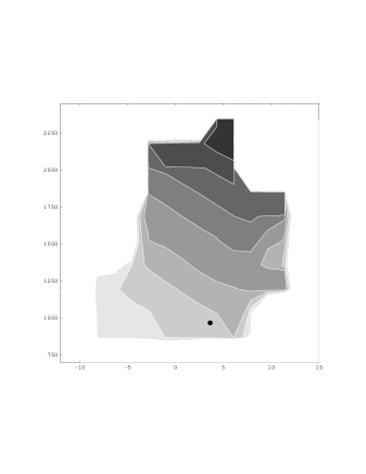
FIG. 4.: Domain of the “good schemes” in the $\widetilde{\gamma}_{1},\widetilde{\gamma}_{2}$ plane. The level curves correspond to values of $\Lambda_{\overline{\rm MS}}$, ranging from $\simeq$ 380 MeV for the darkest down to $\simeq$ 345 MeV. The black circle indicates the position of the $\widetilde{\rm MOM}$ scheme. The $\overline{\rm MS}$ scheme is far outside.

The three conditions (38) and (41) define in the ($\widetilde{\gamma}_{1},\widetilde{\gamma}_{2}$)-parameter space a domain of “good schemes” which is plotted in Fig. 4. The values of $\Lambda_{\overline{\rm MS}}$ vary between $\simeq 345$ MeV and $\simeq 380$ MeV. We will take this as an indication about our systematic uncertainty. However, this is not the whole story. All our analysis has shown that the gluon propagator is not asymptotic at three loops in the present energy range. The range $\simeq 345$ MeV to $\simeq 380$ MeV may be far from the real asymptotic value of $\Lambda_{\overline{\rm MS}}$ but it provides an effective three-loop $\Lambda_{\overline{\rm MS}}^{(3)}$ . It is difficult to estimate the distance of the latter from the former, ignorant as we are of the four-loops coefficients $\beta_{3}$ and $\gamma_{3}$. This distance can be large as we shall illustrate now. We plot in fig. 5(a) the behaviour of $\Lambda_{\overline{\rm MS}}$, computed by obtaining the best fit over the strong coupling constant in the $\widetilde{\rm{MOM}}$ scheme, as a function of the unknown $\beta_{3}$ assuming $\gamma_{3}=0$. As can be seen, a positive $\beta_{3}$ would reduce the value of the four-loop effective $\Lambda_{\overline{\rm MS}}$ compared to the three-loop one. In fig. 5(b) we plot assuming $\beta_{3}=0$ the behaviour of different schemes among our “good schemes” as a function of $\gamma_{3}$: $\widetilde{\gamma}_{3}$ is computed from $\gamma_{3}$ and $\beta_{3}=0$ via eq. (39). We see that their predictions for $\Lambda_{\overline{\rm MS}}$ tend to converge for positive $\gamma_{3}$ where the value of $\Lambda_{\overline{\rm MS}}$ decreases. Of course convergence between the schemes is an indication that we are closer to the correct value of $\gamma_{3}$.

Consequently, we expect that the asymptotic $\Lambda_{\overline{\rm MS}}$ will be smaller than the effective $\Lambda_{\overline{\rm MS}}^{(3)}$ which has been estimated in this work.

FIG. 5.: Plot (a) shows $\Lambda_{\overline{\rm MS}}$ as a function of the unknown $\beta_{3}$ in the $\widetilde{\rm{MOM}}$ scheme assuming $\gamma_{3}=0$. Plot (b) shows three different schemes as a function of $\gamma_{3}$ assuming $\beta_{3}=0$. The solid line if for the $\widetilde{\rm{MOM}}$ scheme. A tendency to converge is seen as $\gamma_{3}$ increases

V Conclusions

Our initial aim has not been fulfilled. We cannot at the present energy scale give a reliable estimate of $\Lambda_{\overline{\rm MS}}$ from the gluon propagator because it has not yet reached its asymptotic regime at three loops ! This is surprising since a scale as large as 5 GeV is often assumed, without further scrutiny, to be large enough to be asymptotic even at two loops ! The $\widetilde{\rm MOM}$ scheme is among our “good schemes”. It is amongst the schemes closest to asymptotic convergence. On the contrary $\overline{\rm MS}$ is very far from convergence.

We have learned an important lesson about the criteria of asymptoticity. It is not enough to have a good fit over a large energy range with an asymptotic formula to check asymptoticity. Our fits are good because the error we introduce by ignoring higher orders is only logarithmic. Our energy range, as large as it may look, corresponds to an increase of $\log q$ by only $\simeq 0.4$. Therefore the higher loops effects can be mimicked by a simple rescaling of $\Lambda_{\overline{\rm MS}}$. The difference in the functional behavior of higher orders would only be apparent on an energy range containing several “e-foldings”, i.e. changes of $\log q$ by several units. Such a study over several “e-foldings” up to a very high scale has been performed in [1].

Combining our results for $\beta=6.2$ and $\beta=6.4$, we end up with the following value for the effective three-loops estimate:

$$\Lambda_{\overline{\rm MS}}^{(3)}=353\pm 2^{+25}_{-10}\,{\rm MeV}$$ (42)

where the first error is statistical and the second is the systematic uncertainty estimated from the scheme dependence.

From a study of the plausible effect of the fourth loop, we have argued that the real asymptotic $\Lambda_{\overline{\rm MS}}$ should lay below the result in eq. (42).

We have discovered that the scheme independence of the result is a much more demanding criterion of asymptoticity than the quality of fit. We have used many “ad hoc” schemes simply defined by a couple of parameters $(\widetilde{\gamma}_{1},\widetilde{\gamma}_{2})$. This technique could be and should be extended to other methods to compute $\alpha_{s}$ and more generally to any program which performs a matching to perturbative QCD, as long as several renormalisation schemes can be used.

Finally we have proposed a new method to eliminate the hypercubic lattice artifacts, namely to take the limit $p^{[4]}\to 0$, eq. (30). We demonstrated that this method is very efficient.

From the result of the present analysis we have undertaken a lattice calculation at smaller lattice spacings, hoping to reach the asymptotic regime.

REFERENCES

• [1] M. Lüscher, Talk given at the 18th International Symposium on Lepton-Photon Interactions, Hamburg, 28 July-1 August 1997; Lecture at l’Ecole des Houches, 28 Jul - 5 Sep 1997; M.Lüscher, R.Sommer, P.Weisz and U. Wolf, Nucl. Phys. B413(1994)481; S. Capitani, M.Lüscher, R.Sommer, H. Wittig, hep-lat/9810063.
• [2] G.S. Bali and K. Schilling, Phys. Rev. D47 (1993) 661.
• [3] G.S.Bali, In Protvino 1993, Problems on high energy physics and field theory 147-163, hep-lat/9311009.
• [4] G.P.Lepage and P. Mackenzie, Phys. Rev. Lett. D48(1992)2250.
• [5] G. de Divitiis et al, Nucl. Phys. B433(1995)390; B437(1995)447.
• [6] B. Alles, D. Henty, H. Panagopoulos, C. Parrinello, C. Pittori, D.G. Richards, Nucl. Phys. B502 (1997) 325; C. Parrinello, Nucl. Phys. Proc. Suppl. 63 (1998) 245; B. Alles, D. Henty, H. Panagopoulos, C. Parrinello, C. Pittori, IFUP-TH-23-96, hep-lat/9605033.
• [7] Ph. Boucaud, J.P. Leroy, J. Micheli, O. Pène and C. Roiesnel, JHEP 10 (98) 017.
• [8] C. Bernard, C. Parrinello and A. Soni, Phys. Rev. D49 (1994) 1585.
• [9] P. Marenzoni, G. Martinelli and N. Stella, Nucl. Phys. B455 (1995) 339; P. Marenzoni, G. Martinelli, N. Stella and M. Testa Phys. Lett. B318 (1993) 511.
• [10] D.B. Leinweber, J.I. Skullerud, A.G. Williams and C. Parrinello, Nucl. Phys. B544 (1999) 669.
• [11] A. Nakamura, S. Sakai, Prog. Theor. Phys. suppl. 131 (1998) 585.
• [12] H. Nakajima, S. Furui, hep-lat/9809078 (Lattice 98),hep-lat/9809081 (Confinement III)
• [13] A. Cucchieri, hep-lat/9902023;hep-lat/9810022 (Lattice 98); A. Cucchieri, T. Mendes, hep-lat/9902024.
• [14] J.P. Ma, hep-lat/9903009.
• [15] S.A. Larin and J.A.M. Vermaseren, Phys. Lett. B303 (1993) 334.
• [16] A.I.Davydychev, P.Osland and O.V.Tarasov, Phys. Rev. D58 (1998) 036007.
• [17] Ph. Boucaud , J.P. Leroy, J. Micheli, O. Pène and C. Roiesnel, JHEP 12 (98) 004.
• [18] G. Grunberg, Phys. Rev. D29 (1984) 2315.
• [19] T.A. Springer, Lecture Notes in Mathematics 585, Springer-verlag (1977).