OHSTPY-HEP-T-98-030
NUHEP-TH-99-73
March 1999

Neutrino Oscillations in a Predictive SUSY GUT

T. Blažek^†‡, S. Raby^∗ and K. Tobe^∗

^†Department of Physics and Astronomy, Northwestern University, Evanston, IL 60208

^∗Department of Physics, The Ohio State University, 174 W. 18th Ave., Columbus, Ohio 43210

Abstract

In this letter we present a predictive SO(10) SUSY GUT with flavor symmetry U(2)$\times$U(1) which has several nice features. We are able to fit fermion masses and mixing angles, including recent neutrino data, with 9 parameters in the charged fermion sector and 4 in the neutrino sector. The flavor symmetry plays a preeminent role –

(i) The model is “natural” – we include all terms allowed by the symmetry. It restricts the number of arbitrary parameters and enforces many zeros in the effective mass matrices.

(ii) Flavor symmetry breaking from U(2)$\times$U(1) $\rightarrow$ U(1) $\rightarrow$ nothing generates the family hierarchy. It also constrains squark and slepton mass matrices, thus ameliorating flavor violation resulting from squark and slepton loop contributions.

(iii) Finally, it naturally gives large angle $\nu_{\mu}-\nu_{\tau}$ mixing describing atmospheric neutrino oscillation data and small angle $\nu_{e}-\nu_{s}$ mixing consistent with the small mixing angle MSW solution to solar neutrino data.

^‡ On leave of absence from Faculty of Mathematics and Physics, Comenius Univ., Bratislava, Slovakia

Abstract

In this letter we present a predictive SO(10) SUSY GUT with flavor symmetry U(2)$\times$U(1) which has several nice features. We are able to fit fermion masses and mixing angles, including recent neutrino data, with 9 parameters in the charged fermion sector and 4 in the neutrino sector. The flavor symmetry plays a preeminent role – (i) The model is “natural” – we include all terms allowed by the symmetry. It restricts the number of arbitrary parameters and enforces many zeros in the effective mass matrices. (ii) Flavor symmetry breaking from U(2)$\times$U(1) $\rightarrow$ U(1) $\rightarrow$ nothing generates the family hierarchy. It also constrains squark and slepton mass matrices, thus ameliorating flavor violation resulting from squark and slepton loop contributions. (iii) Finally, it naturally gives large angle $\nu_{\mu}-\nu_{\tau}$ mixing describing atmospheric neutrino oscillation data and small angle $\nu_{e}-\nu_{s}$ mixing consistent with the small mixing angle MSW solution to solar neutrino data.

1 Introduction

Solar [1], atmospheric [2] and accelerator [3] neutrino data strongly suggest that neutrinos have small masses and non-vanishing mixing angles. This hypothesis is also constrained by reactor [4] based experiments. In the near future, many more experiments will test the hypothesis of neutrino masses. In addition, a neutrino mass necessarily implies new physics beyond the Standard Model. Thus there is great excitement, both experimental and theoretical, in this field.

Phenomenological neutrino mass models [5] are designed to reproduce the best fits to all or some of the neutrino data. These models are only constrained by how much of the neutrino data one wants to fit. Three neutrino models with 3 active neutrinos ($\nu_{e},\;\nu_{\mu}\;\;\rm and\;\;\nu_{\tau}$) are consistent with solar [1] and atmospheric [2] neutrino oscillations, while four neutrino models, including a sterile (or electroweak singlet) neutrino ($\nu_{s}$), are consistent with solar, atmospheric and LSND [3] neutrino experiments. There are also 6 neutrino models, with 3 active and 3 sterile neutrinos, motivated by complete family symmetry [6].

It is important to address the theoretical question; to what extent can this new data on neutrino masses and mixing angles constrain the physics beyond the Standard Model; in particular, theories of fermion masses. Since any number of sterile neutrinos may mix with the 3 active neutrinos, even in a grand unified theory, it may always be possible to fit neutrino data without ever constraining the charged fermion sector of the theory. This would be an unfortunate circumstance. It is the purpose of this paper, however, to show that in any “predictive” theory of charged fermion masses, the neutrino sector is severely constrained.

By a “predictive” model of fermion masses we mean –

• the Lagrangian is “natural” containing all terms consistent with the symmetries and particle content of the theory.

• In addition there are necessarily grand unified [GUT] gauge symmetries as well as family symmetries which restrict the form of the Yukawa matrices [7, 8, 9]; thereby greatly reducing the number of arbitrary parameters.

• In supersymmetric [SUSY] theories, these same family symmetries can usefully constrain the form of soft SUSY breaking squark and slepton masses as well [7, 8, 9]; thus ameliorating the problem of large flavor violation in SUSY [10].

In this letter, we demonstrate that these same family symmetries greatly restrict the form of neutrino masses and mixing. Hence neutrino data can greatly constrain any predictive theory of fermion masses.

We show this in the context of a particular SO(10) SUSY GUT which fits charged fermion masses and mixing angles well. SUSY GUTs are very attractive. They successfully predict the unification of gauge couplings observed at LEP [11, 12]. In SO(10) one family $\{q,\ \bar{u},\ \bar{d},\ l,\ \bar{e},\ \bar{\nu}\}$ fits into the 16 dimensional spinor representation of the group [13]. Thus up, down, charged lepton and Dirac neutrino mass matrices are related.

Of course, the last comment leads to the generic problem for any GUT description of neutrino masses. Atmospheric neutrino data [2] requires large mixing between $\nu_{\mu}$ and $\nu_{x}$, where $\nu_{x}$ is any neutrino species, other than $\nu_{e}$ [2, 4]. Solar neutrino data as well can have a large mixing angle solution. Thus lepton mass matrices must give large mixing angles in sharp contrast to quark mass matrices which give small CKM mixing angles.

We consider an SO(10)$\times$U(2)$\times$U(1) model of fermion masses. This theory is a modification of the SO(10)$\times$U(2) model of Barbieri, Hall, Raby and Romanino [BHRR] [9]. The modifications only affect the results for neutrinos. Alternate descriptions of neutrinos in the context of U(2) family symmetry can be found in recent articles [14]. In section 2, we give the superspace potential and the resulting quark and lepton Yukawa matrices. We then give the results for charged fermion masses and mixing angles. In section 3, we describe the neutrino sector; giving our fits for solar and atmospheric neutrino oscillations and predictions for future experiments. We are not able to accomodate LSND. Our conclusions are in section 4.

2 An SO(10)$\times$U(2)$\times$U(1) model

The three families of fermions are contained in $16_{a},\,a=1,2;$ and $16_{3}$ where $a$ is a U(2) flavor index. [Note U(2) = SU(2) $\times$ U(1)^′ where the U(1)^′ charge is +1 ($-1$) for each upper (lower) SU(2) index.] At tree level, the third family of fermions couples to a $10$ of Higgs with coupling $\lambda\;16_{3}\;10\;16_{3}$ in the superspace potential. The Higgs and $16_{3}$ have zero charge under both U(1)s, while $16_{a}$ has charge $-1$ and thus does not couple to the Higgs at tree level. 

Three superfields ($\phi^{a},\;S^{a\,b}=S^{b\,a},\;A^{a\,b}=-A^{b\,a}$) are introduced to spontaneously break U(2)$\times$U(1) and to generate Yukawa terms giving mass to the first and second generations. The fields ($\phi^{a},\;S^{a\,b},\;A^{a\,b}$) are SO(10) singlets with U(1) charges {0, 1, 2}, respectively. The vacuum expectation values [vevs] ($\phi^{2}\sim S^{2\,2}\sim\epsilon M_{0}^{2}/\langle 45\rangle$) break U(2)$\times$U(1) to $\tilde{U}(1)$ and ($A^{1\,2}\sim\epsilon^{\prime}M_{0}$) completely. In this model, second generation masses are of order $\epsilon$, while first generation masses are of order $\epsilon^{\prime 2}/\epsilon$.

The superspace potential for the charged fermion sector of this theory, including the heavy Froggatt-Nielsen states [15], is given by

$$W\supset 16_{3}\;10\;16_{3}\;\;+\;\;16_{a}\;10\;\chi^{a}$$

$$+\;\;\bar{\chi}_{a}\;(M\;\chi^{a}\;+\;\phi^{a}\;\chi\;+\;S^{a\;b}\;\chi_{b}\;+\;A^{a\;b}\;16_{b})$$

$$+\;\;\bar{\chi}^{a}\;(M^{\prime}\;\chi_{a}\;\;+\;\;45\;16_{a})$$

$$+\;\;\bar{\chi}\;(M^{\prime\prime}\;\chi\;\;+\;\;45\;16_{3})$$

where $M=M_{0}(1\;\;+\;\;\alpha\;X\;\;+\;\;\beta\;Y)$. $X,\;Y$ are SO(10) breaking vevs in the adjoint representation with $X$ corresponding to the U(1) in SO(10) which preserves SU(5), $Y$ is standard weak hypercharge and $\alpha,\;\beta$ are arbitrary parameters. The field $45$ is assumed to obtain a vev in the B - L direction. Note, this theory differs from BHRR [9] in that the fields $\phi^{a}$ and $S^{a\,b}$ are now SO(10) singlets (rather than SO(10) adjoints) and the SO(10) adjoint quantum numbers of these fields, necessary for acceptable masses and mixing angles, has been made explicit in the field $45$ with U(1) charge 1.  This theory thus requires much fewer SO(10) adjoints. Moreover our neutrino mass solution depends heavily on this change.

The effective mass parameters $M_{0},\;M^{\prime},\;M^{\prime\prime}$ are SO(10) invariants. The scales are assumed to satisfy $M_{0}\sim M^{\prime}\sim M^{\prime\prime}\gg\langle\phi^{2}\rangle\sim\langle S^{2\,2}\rangle\gg\langle A^{1\,2}\rangle$ where $M_{0}$ may be of order the GUT scale. In the effective theory below $M_{0}$, the Froggatt-Nielsen states {$\chi,\,\bar{\chi},\ \chi^{a},\,\bar{\chi}_{a},\ \chi_{a},\,\bar{\chi}^{a}$} may be integrated out, resulting in the effective Yukawa matrices for up quarks, down quarks, charged leptons and the Dirac neutrino Yukawa matrix given by (see fig. 1)

$$Y_{u}= \left(\begin{array}[]{ccc}0&\epsilon^{\prime}\rho&0\\ -\epsilon^{\prime}\rho&\epsilon\rho&r\epsilon T_{\bar{u}}\\ 0&r\epsilon T_{Q}&1\end{array}\right)\;\lambda$$ (5)

$$Y_{d}= \left(\begin{array}[]{ccc}0&\epsilon^{\prime}&0\\ -\epsilon^{\prime}&\epsilon&r\sigma\epsilon T_{\bar{d}}\\ 0&r\epsilon T_{Q}&1\end{array}\right)\;\xi$$ (9)

$$Y_{e}= \left(\begin{array}[]{ccc}0&-\epsilon^{\prime}&0\\ \epsilon^{\prime}&3\epsilon&r\epsilon T_{\bar{e}}\\ 0&r\sigma\epsilon T_{L}&1\end{array}\right)\;\xi$$ (13)

$$Y_{\nu}= \left(\begin{array}[]{ccc}0&-\omega\epsilon^{\prime}&0\\ \omega\epsilon^{\prime}&3\omega\epsilon&{1\over 2}\omega r\epsilon T_{\bar{\nu}}\\ 0&r\sigma\epsilon T_{L}&1\end{array}\right)\;\lambda$$ (17)

with

$$\omega={2\,\sigma\over 2\,\sigma-1}$$ (18)

and

$$T_{f}= (\rm Baryon\#-Lepton\#)$$ (19)

$$\rm for f=\{Q,\bar{u},\bar{d},L,\bar{e},\bar{\nu}\}.$$

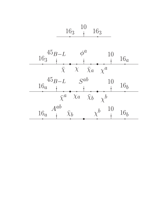
Figure 1: Diagrams generating the Yukawa matrices

In our notation, fermion doublets are on the left and singlets are on the right. Note, we have assumed that the Higgs doublets of the minimal supersymmetric standard model[MSSM] are contained in the $10$ such that $\lambda\;10\supset\lambda\;H_{u}\;+\;\xi\;H_{d}$. We can then consider two important limits — case (1) $\lambda=\xi$ (no Higgs mixing) with large $\tan\beta$, and case (2) $\lambda\gg\xi$ or small $\tan\beta$.

2.1 Results for Charged Fermion Masses and Mixing Angles

Table 1: Charged fermion masses and mixing angles
Initial parameters: large tan$\beta$ case ($\lambda=\xi$)      (1/$\alpha_{G},\,M_{G},\,\epsilon_{3}$) = ($24.52,\,3.05\cdot 10^{16}$ GeV,$\,-4.08$%),
($\lambda,\,$r$,\,\sigma,\,\epsilon,\,\rho,\,\epsilon^{\prime}$) = ($0.79,\,12.4,\,0.84,\,0.011,\,0.043,\,0.0031$),
($\Phi_{\sigma},\,\Phi_{\epsilon},\,\Phi_{\rho}$) = ($0.73,\,-1.21,\,3.72$)rad,
($m_{0},\,M_{1/2},\,A_{0},\,\mu(M_{Z})$) = ($1000,\,300,\,-1437,\,110$) GeV,
($(m_{H_{d}}/m_{0})^{2},\,(m_{H_{u}}/m_{0})^{2},\,$tan$\beta$) = ($2.22,\,1.65,\,53.7$)

$$\begin{array}[]{|l|c|l|}\hline\cr{\rm Observable}&{\rm Data}(\sigma)&Theory\\ \mbox{ }&{\rm(masses}&{\rm in\ \ GeV)}\\ \hline\cr\;\;\;M_{Z}&91.187\ (0.091)&91.17\\ \;\;\;M_{W}&80.388\ (0.080)&80.40\\ \;\;\;G_{\mu}\cdot 10^{5}&1.1664\ (0.0012)&1.166\\ \;\;\;\alpha_{EM}^{-1}&137.04\ (0.14)&137.0\\ \;\;\;\alpha_{s}(M_{Z})&0.1190\ (0.003)&0.1174\\ \;\;\;\rho_{new}\cdot 10^{3}&-1.20\ (1.3)&+0.320\\ \hline\cr\;\;\;M_{t}&173.8\ (5.0)&175.0\\ \;\;\;m_{b}(M_{b})&4.260\ (0.11)&4.328\\ \;\;\;M_{b}-M_{c}&3.400\ (0.2)&3.421\\ \;\;\;m_{s}&0.180\ (0.050)&0.148\\ \;\;\;m_{d}/m_{s}&0.050\ (0.015)&0.0589\\ \;\;\;Q^{-2}&0.00203\ (0.00020)&0.00201\\ \;\;\;M_{\tau}&1.777\ (0.0018)&1.776\\ \;\;\;M_{\mu}&0.10566\ (0.00011)&.1057\\ \;\;\;M_{e}\cdot 10^{3}&0.5110\ (0.00051)&0.5110\\ \;\;\;V_{us}&0.2205\ (0.0026)&0.2205\\ \;\;\;V_{cb}&0.03920\ (0.0030)&0.0403\\ \;\;\;V_{ub}/V_{cb}&0.0800\ (0.02)&0.0691\\ \;\;\;\hat{B}_{K}&0.860\ (0.08)&0.8703\\ \hline\cr{B(b\!\rightarrow\!s\gamma)\!\cdot\!10^{4}}&3.000\ (0.47)&2.995\\ \hline\cr\vrule\lx@intercol{\rm TOTAL}\;\;\;\;\chi^{2}\hfil\lx@intercol 3.39&\\ \hline\cr\end{array}$$

We have performed a global $\chi^{2}$ analysis, incorporating two (one) loop renormalization group[RG] running of dimensionless (dimensionful) parameters from $M_{G}$ to $M_{Z}$ in the MSSM, one loop radiative threshold corrections at $M_{Z}$, and 3 loop QCD (1 loop QED) RG running below $M_{Z}$. Electroweak symmetry breaking is obtained self-consistently from the effective potential at one loop, with all one loop threshold corrections included. This analysis is performed using the code of Blazek et.al. [16].  In this paper, we just present the results for one set of soft SUSY breaking parameters $m_{0},\;M_{1/2}$ with all other parameters varied to obtain the best fit solution. In table 1 we give the 20 observables which enter the $\chi^{2}$ function, their experimental values and the uncertainty $\sigma$ (in parentheses). In most cases $\sigma$ is determined by the 1 standard deviation experimental uncertainty, however in some cases the theoretical uncertainty ($\sim$ 0.1%) inherent in our renormalization group running and one loop threshold corrections dominates.

For large tan$\beta$ there are 6 real Yukawa parameters and 3 complex phases. We take the complex phases to be $\Phi_{\rho},\;\Phi_{\epsilon}$ and $\Phi_{\sigma}$. With 13 fermion mass observables (charged fermion masses and mixing angles [$\hat{B}_{K}$ replacing $\epsilon_{K}$ as a “measure of CP violation”]) we have 4 predictions. For low tan$\beta$ , $\lambda\neq\xi$, we have one less prediction. From table 1 it is clear that this theory fits the low energy data quite well.  Note, fits with $\lambda\gg\xi$ and small $\tan\beta$ fit just as well.

Finally, the squark, slepton, Higgs and gaugino spectrum of our theory is consistent with all available data. The lightest chargino and neutralino are higgsino-like with the masses close to their respective experimental limits. As an example of the additional predictions of this theory consider the CP violating mixing angles which may soon be observed at B factories. For the selected fit we find

$$(\sin 2\alpha,\,\sin 2\beta,\,\sin\gamma)= (0.74,\,0.54,\,0.99)$$ (20)

or equivalently the Wolfenstein parameters

$$(\rho,\,\eta)= (-0.04,\,0.31)$$ . (21)

3 Neutrino Masses and Mixing Angles

The parameters in the Dirac Yukawa matrix for neutrinos (eqn. 9) mixing $\nu-\bar{\nu}$ are now fixed. Of course, neutrino masses are much too large and we need to invoke the GRSY [17] see-saw mechanism.

Since the 16 of SO(10) contains the “right-handed” neutrinos $\bar{\nu}$, one possibility is to obtain $\bar{\nu}-\bar{\nu}$ Majorana masses via higher dimension operators of the form 

$${1\over M}\ \overline{16}\ 16_{3}\ \overline{16}\ 16_{3},$$ (22)

$${1\over M^{2}}\ \overline{16}\ 16_{3}\ \overline{16}\ 16_{a}\ \phi^{a},$$

$${1\over M^{2}}\ \overline{16}\ 16_{a}\ \overline{16}\ 16_{b}\ S^{a\,b}.$$

The second possibility, which we follow, is to introduce SO(10) singlet fields $N$ and obtain effective mass terms $\bar{\nu}-N$ and $N-N$ using only dimension four operators in the superspace potential. To do this, we add three new SO(10) singlets {$N_{a},\;a=1,2;\;\;N_{3}$} with U(1) charges { $-1/2$,  +1/2 }. These then contribute to the superspace potential

$$W\supset \overline{16}\;(N_{a}\;\chi^{a}\;\;+\;\;N_{3}\;16_{3})$$

$$+ {1\over 2}\ N_{a}\;N_{b}\;S^{a\;b}\;\;+\;\;N_{a}\;N_{3}\;\phi^{a}$$ (23)

where the field $\overline{16}$ with U(1) charge $-1/2$ is assumed to get a vev in the “right-handed” neutrino direction. Note, this vev is also needed to break the rank of SO(10).

Finally we allow for the possibility of adding a U(2) doublet of SO(10) singlets $\bar{N}^{a}$ or a U(2) singlet $\bar{N}^{3}$. They enter the superspace potential as follows –

$$W\supset \mu^{\prime}\;N_{a}\;\bar{N}^{a}\;\;+\;\;\mu_{3}\;N_{3}\bar{N}^{3}$$ (24)

The dimensionful parameters $\mu^{\prime},\;\mu_{3}$ are assumed to be of order the weak scale. The notation is suggestive of the similarity between these terms and the $\mu$ term in the Higgs sector. In both cases, we are adding supersymmetric mass terms and in both cases, we need some mechanism to keep these dimensionful parameters small compared to the Planck scale.

We define the 3 $\times$ 3 matrix

$$\tilde{\mu}= \left(\begin{array}[]{ccc}\mu^{\prime}&0&0\\ 0&\mu^{\prime}&0\\ 0&0&\mu_{3}\end{array}\right)$$ (28)

The matrix $\tilde{\mu}$ determines the number of coupled sterile neutrinos, i.e. there are 4 cases labeled by the number of neutrinos ($N_{\nu}=3,4,5,6$):

• ($N_{\nu}=3$)   3 active     ($\mu^{\prime}=\mu_{3}=0$);

• ($N_{\nu}=4$)   3 active + 1 sterile

  ($\mu^{\prime}=0;\;\mu_{3}\neq 0$);

• ($N_{\nu}=5$)   3 active + 2 sterile

  ($\mu^{\prime}\neq 0;\;\mu_{3}=0$);

• ($N_{\nu}=6$)   3 active + 3 sterile

  ($\mu^{\prime}\neq 0;\;\mu_{3}\neq 0$);

In this letter we consider the cases $N_{\nu}=3$ and 4 [18].

The generalized neutrino mass matrix is then given by 

$$(\begin{array}[]{cccc}\;\nu&\;\;\bar{N}&\;\;\bar{\nu}&\;\;N\end{array})$$ (30)

$$\left(\begin{array}[]{cccc}0&0&m&0\\ 0&0&0&\tilde{\mu}^{T}\\ m^{T}&0&0&V\\ 0&\tilde{\mu}&V^{T}&M_{N}\end{array}\right)$$ (35)

where

$$m= Y_{\nu}\;\langle H_{u}^{0}\rangle =\;Y_{\nu}\;{v\over\sqrt{2}}\;\sin\beta$$ (36)

and

$$V= \left(\begin{array}[]{ccc}0&\epsilon^{\prime}V_{16}&0\\ -\epsilon^{\prime}V_{16}&3\epsilon V_{16}&0\\ 0&r\,\epsilon\,(1-\sigma)\,T_{\bar{\nu}}V_{16}&V^{\prime}_{16}\end{array}\right)$$ (40)

$$M_{N}= \left(\begin{array}[]{ccc}0&0&0\\ 0&S&\phi\\ 0&\phi&0\end{array}\right)$$ (44)

$V_{16},\;V^{\prime}_{16}$ are proportional to the vev of $\overline{16}$ (with different implicit Yukawa couplings) and $S,\;\phi$ are up to couplings the vevs of $S^{22},\;\phi^{2}$, respectively.

Since both $V$ and $M_{N}$ are of order the GUT scale, the states $\bar{\nu},\;N$ may be integrated out of the effective low energy theory. In this case, the effective neutrino mass matrix is given (at $M_{G}$) by  (the matrix is written in the ($\nu,\ \bar{N}$) flavor basis where charged lepton masses are diagonal)

$$m_{\nu}=$$ (45)

$$\tilde{U}_{e}^{T}\;\left(\begin{array}[]{cc}m\;(V^{T})^{-1}\;M_{N}\;V^{-1}\;m^{T}&-m\;(V^{T})^{-1}\;\tilde{\mu}\\ -{\tilde{\mu}}^{T}\;V^{-1}\;m^{T}&0\end{array}\right)\;\tilde{U}_{e}$$ (48)

with

$$\tilde{U}_{e}= \left(\begin{array}[]{cc}U_{e}&0\\ 0&1\end{array}\right)$$ (51)

$$e_{0}=U_{e}\;e\;\;; \nu_{0}=U_{e}\;\nu$$

$U_{e}$ is the $3\times 3$ unitary matrix for left-handed leptons needed to diagonalize $Y_{e}$ (eqn. 9) and $e_{0},\;\nu_{0}\;(e,\;\nu)$ represent the three families of left-handed leptons in the charged-weak ( -mass) eigenstate basis.

The neutrino mass matrix is diagonalized by a unitary matrix $U=U_{\alpha\,i}$;

$$m^{diag}_{\nu}= U^{T}\;m_{\nu}\;U$$ (52)

where $\alpha=\{\nu_{e},\;\nu_{\mu},\;\nu_{\tau},\;\nu_{s_{1}},\;\nu_{s_{2}},\;\nu_{s_{3}}\}$ is the flavor index and $i=\{1,\cdots,6\}$ is the neutrino mass eigenstate index. $U_{\alpha\,i}$ is observable in neutrino oscillation experiments. In particular, the probability for the flavor state $\nu_{\alpha}$ with energy $E$ to oscillate into $\nu_{\beta}$ after travelling a distance $L$ is given by

$$P(\nu_{\alpha}\rightarrow\nu_{\beta})=$$ (53)

$$\delta_{\alpha\beta}-4\sum_{k\;<\,j}U_{\alpha\,k}\ U^{*}_{\beta\,k}\ U^{*}_{\alpha\,j}\ U_{\beta\,j}\ \sin^{2}\Delta_{j\,k}$$

where $\Delta_{j\,k}={\delta m^{2}_{jk}\ L\over 4E}$ and $\delta m^{2}_{jk}=m^{2}_{j}-m^{2}_{k}$.

In general, neutrino masses and mixing angles have many new parameters so that one might expect to have little predictability. However, as we shall now see, the U(2)$\times$U(1) flavor symmetry of the theory provides a powerful constraint on the form of the neutrino mass matrix. In particular, the matrix has many zeros and few arbitrary parameters. Before discussing the four neutrino case, we show why 3 neutrinos cannot work without changing the model.

3.1 Three neutrinos

Consider first $m_{\nu}$ for three active neutrinos. We find (at $M_{G}$) in the ($\nu_{e},\;\nu_{\mu},\;\nu_{\tau}$) basis

$$m_{\nu}=m^{\prime}\;U_{e}^{T}\;\left(\begin{array}[]{ccc}0&0&0\\ 0&b&1\\ 0&1&0\end{array}\right)\;U_{e}$$ (57)

with

$$m^{\prime} = \frac{\lambda^{2}v^{2}\sin^{2}\beta~{}\omega\phi}{2V_{16}V^{\prime}_{16}}\approx{m_{t}^{2}\ \omega\ \phi\over V_{16}\ V^{\prime}_{16}}$$ (58)

$$b = \omega\ {S\ V^{\prime}_{16}\over\phi\ V_{16}}+2\ \sigma\ r\ \epsilon$$

where in the approximation for $m^{\prime}$ we use

$$m_{t}(\equiv m_{top})\approx\lambda\ {v\over\sqrt{2}}\ \sin\beta,$$ (59)

valid at the weak scale.

$m_{\nu}$ is given in terms of two independent parameters { $m^{\prime},\;b$ }. Note, this theory in principle solves two problems associated with neutrino masses. It naturally has small mixing between $\nu_{e}-\nu_{\mu}$ since the mixing angle comes purely from diagonalizing the charged lepton mass matrix which, like quarks, has small mixing angles. While, for $b\leq 1$, $\nu_{\mu}-\nu_{\tau}$ mixing is large without fine tuning. Also note, in this theory one neutrino (predominantly $\nu_{e}$) is massless.

Unfortunately this theory cannot simultaneously fit both solar and atmospheric neutrino data. This problem can be solved at the expense of adding a new flavor symmetry breaking vev 

$$\langle\phi^{1}\rangle=\kappa\langle\phi^{2}\rangle.$$ (60)

We discuss this three neutrino solution in a future paper [18]. With $\kappa\neq 0$ the massless eigenvalue in the neutrino mass matrix is now lifted. This allows us to obtain a small mass difference between the first and second mass eigenvalues which was unattainable before in the large mixing limit for $\nu_{\mu}-\nu_{\tau}$. Hence a good fit to both solar and atmospheric neutrino data can now be found for $\kappa\leq 0.2$. In addition, note that this small value of $\kappa$ moderately improves the global fits to charged fermion masses and mixing angles[18].

In the next section we discuss a four neutrino solution to both solar and atmospheric neutrino oscillations in the theory with $\kappa=0$.

3.2 Neutrino oscillations [ 3 active + 1 sterile ]

In the four neutrino case the mass matrix (at $M_{G}$) is given by 

$$m^{\prime}\ \left[\begin{array}[]{cccc}U_{e}^{T}\,\left(\begin{array}[]{ccc}0&0&0\\ 0&b&1\\ 0&1&0\end{array}\right)\,U_{e}&-U_{e}^{T}\left(\begin{array}[]{c}0\\ u\,c\\ c\end{array}\right)\\ -\left(\begin{array}[]{ccc}0&u\,c&c\end{array}\right)\,U_{e}&0\end{array}\right]$$ (70)

where $m^{\prime}$ and $b$ are given in eqn. 58 and

$$u = \sigma\,r\,\epsilon$$ (71)

$$c = {\sqrt{2}\ \mu_{3}\,V_{16}\over\omega\,\lambda\ v\ \sin\beta\ \phi}\approx{\mu_{3}\,V_{16}\over\omega\,m_{t}\ \phi}$$

In the analysis of neutrino masses and mixing angles we use the fits for charged fermion masses as input. Thus the parameter $u$ is fixed. We then look for the best fit to solar and atmospheric neutrino oscillations. For this we use the latest Super-Kamiokande data for atmospheric neutrino oscillations [2] and the best fits to solar neutrino data including the possibility of “just so” vacuum oscillations or both large and small angle MSW oscillations [1]. Our best fit is found in tables 2 and 3. It is obtained in the following way.

For atmospheric neutrino oscillations we have evaluated the probabilities ($P(\nu_{\mu}\rightarrow\nu_{\mu})$, $P(\nu_{\mu}\rightarrow\nu_{x})\ {\rm with}\ x=\{e,\ \tau,\ s\}$) as a function of ${\rm x}\equiv\rm{Log}[(L/km)/(E/GeV)]$. In order to smooth out the oscillations we have averaged the result over a bin size, $\Delta$x = 0.5. In fig. 2a we have compared the results of our model with a 2 neutrino oscillation model. We see that our result is in good agreement with the values of $\delta m^{2}_{atm}$ and $\sin^{2}2\theta_{atm}$ as given.

An approximate formula for the effective atmospheric mixing angle is defined by

$$P(\nu_{\mu}\rightarrow\nu_{\mu})\equiv 1-`\sin^{2}2\theta_{atm}`\sin^{2}({`\delta m^{2}_{atm}`\ \rm L\over 4\ E})$$ (72)

with

$$`\sin^{2}2\theta_{atm}` \approx 4\ [\ \|U_{\mu 4}\|^{2}(1-\|U_{\mu 4}\|^{2})$$

$$+ \|U_{\mu 3}\|^{2}(1-\|U_{\mu 3}\|^{2}-\|U_{\mu 4}\|^{2})\ ]$$

using the approximate relation

$$`\delta m^{2}_{atm}`=\delta m^{2}_{43}\approx\delta m^{2}_{42}\approx\delta m^{2}_{41}\approx\delta m^{2}_{32}\approx\delta m^{2}_{31}.$$ (74)

Note, $`\sin^{2}2\theta_{atm}`$ may be greater than one. This is consistent with the definition above and also with Super-Kamiokande data where the best fit occurs for $\sin^{2}2\theta_{atm}=1.05$. We obtain a good fit to the data.

In fig. 2b we see however that although the atmospheric neutrino deficit is predominantly due to the maximal mixing between $\nu_{\mu}-\nu_{\tau}$, there is nevertheless a significant ($\sim$ 10% effect) oscillation of $\nu_{\mu}-\nu_{s}$. This effect may be observable at Super-Kamiokande. It would appear as a deficit of neutrinos in the ratio of experimental to theoretical muon (single ring events) plus tau (multi-ring events) as a function of $L/E$.

The oscillations $\nu_{\mu}\rightarrow\nu_{\tau}$ or $\nu_{s}$ may also be visible at long baseline neutrino experiments. For example at K2K [20], the mean neutrino energy $E=1.4$GeV and distance $L=250$ km corresponds to a value of x = 2.3 in fig. 2b and hence $P(\nu_{\mu}\rightarrow\nu_{\tau})\sim.4$ and $P(\nu_{\mu}\rightarrow\nu_{s})\sim.1$. At Minos [21] low energy beams with hybrid emulsion detectors are also being considered. These experiments can first test the hypothesis of muon neutrino oscillations by looking for muon neutrino disappearance (for x = 2.3 we have $P(\nu_{\mu}\rightarrow\nu_{\mu})\sim.5$). Verifying oscillations into sterile neutrinos is however much more difficult. For example at K2K, if only quasi-elastic muon neutrino interactions (single ring events at SuperK) are used, then this cannot be tested. Minos, on the other hand, may be able to verify the oscillations into sterile neutrinos by using the ratio of neutral current to charged current measurements [21] (the so-called T test).

Table 2: Fit to atmospheric and solar neutrino
oscillations
Initial parameters: ( 4 neutrinos   $w$/ large tan$\beta$ )     $m^{\prime}=7.11\cdot 10^{-2}$ eV ,  $b$ = $-0.521$,  $c$ = 0.278, $\Phi_{b}$ = 3.40rad

$$\begin{array}[]{|c|c|}\hline\cr{\rm Observable}&{\rm Computed\;\;value}\\ \hline\cr\delta m^{2}_{atm}&3.2\cdot 10^{-3}\ \rm eV^{2}\\ \sin^{2}2\theta_{atm}&1.08\\ \delta m^{2}_{sol}&4.2\cdot 10^{-6}\ \rm eV^{2}\\ \sin^{2}2\theta_{sol}&3.0\cdot 10^{-3}\\ \hline\cr\end{array}$$

Table 3: Neutrino Masses and Mixings           
Mass eigenvalues [eV]:    0.0,  0.002,  0.04,  0.07          
Magnitude of neutrino mixing matrix U_αi                
$i=1,\cdots,4$ – labels mass eigenstates.              
$\alpha=\{e,\ \mu,\ \tau,\ s\}$ labels flavor eigenstates.

$$\left[\begin{array}[]{cccc}0.998&0.0204&0.0392&0.0529\\ 0.0689&0.291&0.567&0.767\\ 0.317\cdot 10^{-3}&0.145&0.771&0.620\\ 0.284\cdot 10^{-3}&0.946&0.287&0.154\\ \end{array}\right]$$

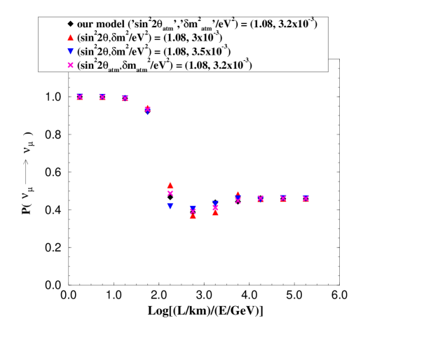
Figure 2 a: Probability $P(\nu_{\mu}\longrightarrow\nu_{\mu})$ for atmospheric neutrinos. For this analysis, we neglect the matter effects.

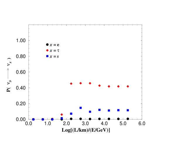
Figure 2 b: Probabilities $P(\nu_{\mu}\longrightarrow\nu_{x})$ ($x=e$, $\tau$ and $s$) for atmospheric neutrinos

For solar neutrinos we plot, in figs. 3(a,b), the probabilities ($P(\nu_{e}\rightarrow\nu_{e})$, $P(\nu_{e}\rightarrow\nu_{x})\ {\rm with}\ x=\{\mu,\ \tau,\ s\}$) for neutrinos produced at the center of the sun to propagate to the surface (and then without change to earth), as a function of the neutrino energy E_ν (MeV).  We compare our model to a 2 neutrino oscillation model with the given parameters. We see that the solar neutrino deficit is predominantly due to the small mixing angle MSW solution for $\nu_{e}-\nu_{s}$ oscillations. The results are summarized in tables 2 and 3.

A naive definition of the effective solar mixing angle is given by

$$\sin^{2}2\theta_{12}\equiv 4\ \|U_{e1}\|^{2}\ \|U_{e2}\|^{2}.$$ (75)

In fig. 3a we see that the naive definition of $\sin^{2}2\theta_{12}$ underestimates the value of the effective 2 neutrino mixing angle. Thus we see that our model reproduces the neutrino results for $\delta m^{2}_{sol}=\delta m^{2}_{12}=4.2\times 10^{-6}$ eV² but instead is equivalent to a 2 neutrino mixing angle $\sin^{2}2\theta_{sol}=3\times 10^{-3}$ instead of $\sin^{2}2\theta_{12}=1.6\times 10^{-3}$. Our result is consistent with the fits of Bahcall et al. [1].

In addition, whereas the oscillation $\nu_{e}-\nu_{s}$ dominates we see in fig 3b that there is a sigificant ($\sim$ 8% effect) for $\nu_{e}-\nu_{\mu}$. This result may be observable at SNO [22] with threshold $E\geq 5$ MeV for which $P(\nu_{e}\rightarrow\nu_{\mu})\sim.05$.

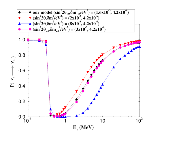
Figure 3 a: Probability $P(\nu_{e}\longrightarrow\nu_{e})$ for solar neutrinos

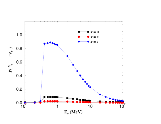
Figure 3 b: Probabilities $P(\nu_{e}\longrightarrow\nu_{x})$ ($x=\mu$, $\tau$ and $s$) for solar neutrinos

We note that, even though we have four neutrinos, we are not able to simultaneously fit atmospheric, solar and LSND data, i.e. it is not possible to get $``\delta m^{2}_{\nu_{e}-\nu_{\mu}}"$ large enough to be consistent with LSND. We have also checked that introducing the new parameter $\kappa$ (eqn. 60) does not help.

Finally let’s discuss whether the parameters necessary for the fit make sense. We have three arbitrary parameters. We have taken $b$ complex, while any phases for $m^{\prime}$ and $c$ are unobservable. A large mixing angle for $\nu_{\mu}-\nu_{\tau}$ oscillations is obtained with $|b|\sim 0.5$. This does not require any fine tuning; it is consistent with ${S\ V^{\prime}_{16}\over\phi\ V_{16}}\sim 1$ which is perfectly natural (see eqn. 58). The parameter $c[\rm{eqn.}\ref{eq:c}]\approx 0.28\approx{\mu_{3}\,V_{16}\over\omega\,m_{t}\ \phi}$ implies $\mu_{3}\approx 0.41\ {\phi\over V_{16}}\ m_{t}$. Thus in order to have a light sterile neutrino we need the parameter $\mu_{3}\sim 110$ GeV for $\phi\sim V_{16}$. Considering that the standard $\mu$ parameter (see the parameter list in the captions to table 1) with value $\mu=110$ GeV and $\mu_{3}$ [eqn. 24] may have similar origins, both generated once SUSY is spontaneously broken, we feel that it is natural to have a light sterile neutrino. Lastly consider the overall scale of symmetry breaking, i.e. the see-saw scale. We have $m^{\prime}=7\times 10^{-2}\rm eV[table~{}\ref{t:4numass2}]\approx{m_{t}^{2}\ \omega\ \phi\over V_{16}\ V^{\prime}_{16}}$. Thus we find ${V_{16}\ V^{\prime}_{16}\over\phi}\sim{m_{t}^{2}\ \omega\over m^{\prime}}\sim 1.6\times 10^{15}$ GeV. This is perfectly reasonable for $\langle\overline{16}\rangle\sim\langle\phi^{2}\rangle\sim M_{G}$ once the implicit Yukawa couplings are taken into account.

4 Conclusion

We have presented the results of a predictive SO(10)$\times$U(2)$\times$U(1) model of fermion masses. We fit charged fermion masses and mixing angles as well as neutrino masses and mixing. The model “naturally” gives small mixing angles for charged fermions and for $\nu_{e}\rightarrow\nu_{sterile}$ oscillations (small angle MSW solution to solar neutrino problem) and large mixing angle for $\nu_{\mu}\rightarrow\nu_{\tau}$ oscillations (atmospheric muon neutrino deficit). The model presented here may be one of a large class of models which fit charged fermion masses. The most important conclusion from our work is that predictive theories of charged fermion masses (including GUT and family symmetry) strongly constrain the neutrino sector of the theory. These theories can thus be predictive in the neutrino sector and neutrino data will strongly constrain any predictive theory of fermion masses.

Acknowledgements Finally, S.R. and K.T. are partially supported by DOE grant DOE/ER/01545-761.

References

- [1] J.N. Bahcall, P.I. Krastev and A. Yu. Smirnov, Phys. Rev.D58 096016 (1998) and references therein.
- [2] The Super-Kamiokande Collaboration, Phys. Rev. Lett. 81 1562 (1998).
- [3] LSND Collaboration, C. Athanassopoulos et al., Phys. Rev. Lett.81 1774 (1998); ibid., Phys. Rev.C58 2489 (1998).
- [4] CHOOZ Collaboration, M. Apollonio et al., Phys.Lett. B420 397 (1998).
- [5] G. Altarelli and F. Feruglio, Jour. of HEP9811 021 (1998); V. Barger, S. Pakvasa, T.J. Weiler and K. Whisnant, Phys. Lett.B437 107 (1998); R. Barbieri, L.J. Hall, D. Smith, A. Strumia and N. Weiner, hep-ph/9807235; R.N. Mohapatra and S. Nussinov, hep-ph/9808301 ; V. Barger,hep-ph/9808353; V. Barger and K. Whisnant, hep-ph/9812273.
- [6] A. Geiser, Phys. Lett.B444 358 (1999).
- [7] L.J. Hall and L. Randall, Phys. Rev. Lett.65 2939 (1990); M. Dine, R. Leigh and A. Kagan, Phys. Rev.D48 4269 (1993); Y. Nir and N. Seiberg, Phys. Lett.B309 337 (1993); P. Pouliot and N. Seiberg, Phys. Lett.B318 169 (1993); M. Leurer, Y. Nir and N. Seiberg, Nucl. Phys.B398 319 (1993); M. Leurer, Y. Nir and N. Seiberg, Nucl. Phys.B420 468 (1994); D. Kaplan and M. Schmaltz, Phys. Rev.D49 3741 (1994); A. Pomarol and D. Tommasini, Nucl.Phys.B466 3 (1996); L.J. Hall and H. Murayama, Phys. Rev. Lett.75 3985 (1995); P. Frampton and O. Kong, Phys. Rev. Lett.75 781 (1995) and ibid., Phys.Rev.D53 2293 (1996); E. Dudas, S. Pokorski and C.A. Savoy, Phys. Lett.B356 45 (1995) and ibid., Phys. Lett.B369 255 (1996); C. Carone, L.J. Hall and H. Murayama, Phys. Rev.D53 6282 (1996); P. Binetruy, S. Lavignac and P. Ramond, Nucl. Phys.B477 353 (1996); V. Lucas and S. Raby, Phys. Rev.D54 2261 (1996); Z. Berezhiani, Phys.Lett. B417 287 (1998).
- [8] M. Dine, R. Leigh and A. Kagan, Phys. Rev.D48 4269 (1993); A. Pomarol and D. Tommasini, Nucl.Phys.B466 3 (1996); R. Barbieri, G. Dvali and L.J. Hall, Phys. Lett.B377 76 (1996); R. Barbieri and L.J. Hall, Nuovo Cim.110A 1 (1997).
- [9] R. Barbieri, L.J. Hall, S. Raby and A. Romanino, Nucl. Phys.B493 3 (1997); R. Barbieri, L.J. Hall and A. Romanino, Phys. Lett.B401 47 (1997).
- [10] S. Dimopoulos and H. Georgi, Nucl. Phys. B193 150 (1981); L.J. Hall, V.A. Kostelecky and S. Raby, Nucl. Phys.B267 415 (1986); H. Georgi, Phys.Lett.169B 231 (1986); F. Borzumati and A. Masiero, Phys. Rev. Lett.57 961 (1986); R. Barbieri and L.J. Hall, Phys. Lett. B338 212 (1994); R. Barbieri, L.J. Hall and A. Strumia, Nucl. Phys.B445 219 (1995); J. Hisano, T. Moroi, K. Tobe, M. Yamaguchi and T. Yanagida, Phys. Lett.B357 579 (1995); F. Gabbiani, E. Gabrielli, A. Masiero and L. Silvestrini, Nucl. Phys.B477 321 (1996); S. Dimopoulos and A. Pomarol, Phys. Lett.B353 222 (1995); J. Hisano, T. Moroi, K. Tobe and M. Yamaguchi, Phys. Rev. D53 2442 (1996); ibid., Phys. Lett. B391 341 (1997); K. Tobe, Nucl. Phys. (Proc. Suppl.) B59, 223 (1997); J. Hisano, D. Nomura, T. Yanagida, Phys. Lett.B437 351 (1998); J. Hisano, D. Nomura, Y. Okada, Y. Shimizu, M. Tanaka, Phys. Rev. D58 116010 (1998); J. Hisano and D. Nomura, hep-ph/9810479.
- [11] S. Dimopoulos, S. Raby and F. Wilczek, Phys. Rev.D24 1681 (1981); S. Dimopoulos and H. Georgi, Nucl. Phys.B193 150 (1981).
- [12] For more recent tests of gauge coupling unifications, see P. Langacker and N. Polonsky, Phys. Rev.D52 3081 (1995); P.H. Chankowski, Z. Pluciennik, S. Pokorski, Nucl. Phys. B439 23 (1995).
- [13] H. Georgi, Particles and Fields, Proceedings of the APS Div. of Particles and Fields, ed C. Carlson; H. Fritzsch and P. Minkowski, Ann. Phys. 93, 193 (1975).
- [14] C.D. Carone and L.J. Hall, Phys.Rev.D56 4198 (1997); L.J. Hall and N. Weiner, hep-ph/9811299.
- [15] C. Froggatt and H.B. Nielsen, Nucl. Phys.B147 277 (1979).
- [16] T. Blazek, M. Carena, S. Raby and C. Wagner, Phys. Rev.D56 6919 (1997).
- [17] M. Gell-Mann, P. Ramond and R. Slansky, in Supergravity, ed. P. van Nieuwenhuizen and D.Z. Freedman, North-Holland, Amsterdam, 1979, p. 315 ; T. Yanagida, in Proceedings of the Workshop on the unified theory and the baryon number of the universe, ed. O. Sawada and A. Sugamoto, KEK report No. 79-18, Tsukuba, Japan, 1979.
- [18] T. Blazek, S. Raby and K. Tobe, a paper describing our results for with or is in preparation.
- [19] R.N. Mohapatra and J.W.F. Valle, Phys. Rev.D34 1634 (1986).
- [20] M. Sakuda (K2K Collaboration), “The KEK-PS Long Baseline Neutrino Oscillation Experiment (E362)”, KEK-PREPRINT-97-254; Yuichi Oyama (K2K Collaboration) “K2K (KEK To Kamioka) Neutrino-Oscillation Experiment At KEK-PS”, KEK-PREPRINT-97-266 (hep-ex/9803014).
- [21] MINOS Collaboration, “Neutrino Oscillation Physics at Fermilab: The NuMI-MINOS Project”, NuMI-L-375. See also the MINOS web page: http://www.hep.anl.gov/ndk/hypertext/numi.html.
- [22] M.E. Moorhead (SNO Collaboration), Nucl. Phys. (Proc. Suppl.) B48, 378 (1996).