Anomalous Quartic Couplings
in $W^{+}W^{-}\gamma$, $Z^{0}Z^{0}\gamma$ and $Z^{0}\gamma\gamma$ Production
at Present and Future $e^{+}e^{-}$ Colliders

W. James Stirling^1,2 and Anja Werthenbach¹
1) Department of Physics, University of Durham, Durham DH1 3LE, U.K.

2) Department of Mathematical Sciences, University of Durham, Durham DH1 3LE, U.K.

Abstract

The production of three electroweak gauge bosons in high-energy $e^{+}e^{-}$ collisions offers a window on anomalous quartic gauge boson couplings. We investigate the effect of three possible anomalous couplings on the cross sections for $W^{+}W^{-}\gamma$, $Z^{0}Z^{0}\gamma$ and $Z^{0}\gamma\gamma$ productions at LEP2 ($\sqrt{s}=200$ GeV) and at a future linear collider ($\sqrt{s}=500$ GeV). We find that the combination of energies and processes provides reasonable discrimination between the various anomalous contributions.

1 Introduction

In the Standard Model (SM), the couplings of the gauge bosons and fermions are tightly constrained by the requirements of gauge symmetry. In the electroweak sector, for example, this leads to trilinear $VVV$ and quartic $VVVV$ interactions between the gauge bosons $V=\gamma,Z^{0},W^{\pm}$ with completely specified couplings. Electroweak symmetry breaking via the Higgs mechanism gives rise to additional Higgs – gauge boson interactions, again with specified couplings.

The trilinear and quartic gauge boson couplings probe different aspects of the weak interactions. The trilinear couplings directly test the non-Abelian gauge structure, and possible deviations from the SM forms have been extensively studied in the literature, see for example [1] and references therein. Experimental bounds have also been obtained [2]. In contrast, the quartic couplings can be regarded as a more direct window on electroweak symmetry breaking, in particular to the scalar sector of the theory (see for example [3]) or, more generally, on new physics which couples to electroweak bosons.

In this respect it is quite possible that the quartic couplings deviate from their SM values while the triple gauge vertices do not. For example, if the mechanism for electroweak symmetry breaking does not reveal itself through the discovery of new particles such as the Higgs boson, supersymmetric particles or technipions it is possible that anomalous quartic couplings could provide the first evidence of new physics in this sector of the electroweak theory [3].

High-energy colliders provide the natural environment for studying anomalous quartic couplings. The paradigm process is $f\bar{f}\to VVV$, with $f=e$ ($e^{+}e^{-}$ colliders) or $f=q$ (hadron-hadron colliders), where one of the Feynman diagrams corresponds to $f\bar{f}\to V^{*}\to VVV$. In this context, one may consider the quartic-coupling diagram(s) as the signal, while the remaining diagrams constituting the background. The sensitivity of a given process to anomalous quartic couplings depends on the relative importance of these two types of contribution, as we shall see.

In this study we shall focus on $e^{+}e^{-}$ collisions, and quantify the dependence of various $e^{+}e^{-}\to VVV$ cross sections on the anomalous couplings. We shall consider in particular $\sqrt{s}=200$ and $500$ GeV, corresponding to LEP2 and a future linear collider (LC) respectively. For obvious kinematic reasons, processes where at least one of the gauge bosons is a photon have the largest cross sections. Indeed, $VVV$ production with $V=Z^{0},W^{\pm}$ are kinematically forbidden at 200 GeV and suppressed at 500 GeV. We therefore consider $W^{+}W^{-}\gamma$, $Z^{0}Z^{0}\gamma$ and $Z^{0}\gamma\gamma$ production. Each of these contains at least one type of quartic interaction.

There have been several studies of this type reported in the literature [4, 5]. Our aim is partly to complete as well as update these, and partly to assess the relative merits of the above-mentioned processes in providing information on the anomalous couplings. Note that our primary interest is in the so-called ‘genuine’ anomalous quartic couplings, i.e. those which give no contribution to the trilinear vertices.

In the following section we review the various types of anomalous quartic coupling that might be expected in extensions of the SM. In Section 3 we present numerical studies illustrating the impact of the anomalous couplings on various $VVV$ cross sections. Finally in Section 4 we present our conclusions.

2 Anomalous gauge boson couplings

The lowest dimension operators which lead to genuine quartic couplings where at least one photon is involved are of dimension 6 [4]. A dimension 4 operator is not realised since a custodial $SU(2)$ symmetry is required to keep the $\rho$ parameter, $\rho=M_{W}^{2}/(M_{Z}^{2}\cos^{2}\theta_{w})$, close to its measured SM value of 1. Thus the 4-dimensional operator

$${\cal L}_{4}=-\frac{1}{4}\,g^{2}(\stackrel{{\scriptstyle\longrightarrow}}{{W_{\mu}}}\times\stackrel{{\scriptstyle\longrightarrow}}{{W_{\nu}}})\,(\stackrel{{\scriptstyle\longrightarrow}}{{W^{\mu}}}\times\stackrel{{\scriptstyle\longrightarrow}}{{W^{\nu}}})$$ (1)

with

$$\stackrel{{\scriptstyle\longrightarrow}}{{W_{\mu}}}=\left(\begin{array}[]{c}\frac{1}{\sqrt{2}}(W_{\mu}^{+}+W_{\mu}^{-})\\ \frac{i}{\sqrt{2}}(W_{\mu}^{+}-W_{\mu}^{-})\\ W_{\mu}^{3}-\frac{g^{\prime}}{g}B_{\mu}\end{array}\right)$$ (5)

and

$$W_{\mu}^{3}-\frac{g^{\prime}}{g}B_{\mu} = \cos\theta_{w}\,Z_{\mu}+\sin\theta_{w}A_{\mu}-\frac{e}{\cos\theta_{w}}\frac{\sin\theta_{w}}{e}(-\sin\theta_{w}Z_{\mu}+\cos\theta_{w}A_{\mu})$$ (6)

$$= \frac{Z_{\mu}}{\cos\theta_{w}}\ .$$

does not involve the photon field $A_{\mu}$. The other possible 4-dimensional operator [4]

$$\widetilde{{\cal L}_{4}}=-ie\frac{\lambda_{\gamma}}{M_{W}^{2}}\,F^{\mu\nu}W_{\mu\alpha}^{\dagger}W^{\alpha}_{\phantom{\alpha}\nu}$$ (7)

with

$$F^{\mu\nu} = \partial_{\mu}A_{\nu}-\partial_{\nu}A_{\mu}$$

$$W_{\mu\nu} = \partial_{\mu}\mbox{\bf W}_{\nu}-\partial_{\nu}\mbox{\bf W}_{\mu}-g\mbox{\bf W}_{\mu}\times\mbox{\bf W}_{\nu}$$ (8)

and

$$\mbox{\bf W}_{\mu}=\left(\begin{array}[]{c}\frac{1}{\sqrt{2}}(W_{\mu}^{+}+W_{\mu}^{-})\\ \frac{i}{\sqrt{2}}(W_{\mu}^{+}-W_{\mu}^{-})\\ \cos\theta_{w}Z_{\mu}+\sin\theta_{w}A_{\mu}\end{array}\right)\ ,$$ (12)

generates trilinear couplings in addition to quartic ones and is therefore not ‘genuine’. In Section 4 we will briefly discuss the impact of possible non-zero anomalous trilinear couplings on our analysis.

We are therefore left with several 6-dimensional operators. First the neutral and the charged Lagrangians, both giving anomalous contributions to the $VV\gamma\gamma$ vertex, with $VV$ either being $W^{+}W^{-}$ or $Z^{0}Z^{0}$.

$${\cal L}_{0} = -\frac{e^{2}}{16\Lambda^{2}}\,a_{0}\,F^{\mu\nu}\,F_{\mu\nu}\stackrel{{\scriptstyle\longrightarrow}}{{W^{\alpha}}}\cdot\stackrel{{\scriptstyle\longrightarrow}}{{W_{\alpha}}}$$ (13)

$$= -\frac{e^{2}}{16\Lambda^{2}}\,a_{0}\,\big{[}-2(p_{1}\cdot p_{2})(A\cdot A)+2(p_{1}\cdot A)(p_{2}\cdot A)\big{]}$$

$$\hskip 42.67912pt{\scriptscriptstyle\times}\big{[}2(W^{+}\cdot W^{-})+(Z\cdot Z)/\cos^{2}\theta_{w}\big{]}\quad,$$

$${\cal L}_{c} = -\frac{e^{2}}{16\Lambda^{2}}\,a_{c}\,F^{\mu\alpha}\,F_{\mu\beta}\stackrel{{\scriptstyle\longrightarrow}}{{W^{\beta}}}\cdot\stackrel{{\scriptstyle\longrightarrow}}{{W_{\alpha}}}$$ (14)

$$= -\frac{e^{2}}{16\Lambda^{2}}\,a_{c}\,\big{[}-(p_{1}\cdot p_{2})\,A^{\alpha}A_{\beta}+(p_{1}\cdot A)\,A^{\alpha}p_{2\beta}\big{.}$$

$$\hskip 51.21504pt\big{.}\quad\quad+(p_{2}\cdot A)\,p_{1}^{\alpha}A_{\beta}-(A\cdot A)\,p_{1}^{\alpha}p_{2\beta}\big{]}$$

$$\hskip 42.67912pt{\scriptscriptstyle\times}\big{[}W_{\alpha}^{-}W^{+\beta}+W_{\alpha}^{+}W^{-\beta}+Z_{\alpha}Z^{\beta}/{\cos^{2}\theta_{w}}\big{]}\ .$$

where $p_{1}$ and $p_{2}$ are the photon momenta.

Since we are interested in the anomalous $VV\gamma\gamma$ contribution we pick up the corresponding part of the Lagrangian. To obtain the Feynman rules for the corresponding vertex (in agreement with [6]) we have to multiply by 2 for the two identical photons (as well as for the $Z^{0}$s in the case of $VV=Z^{0}Z^{0}$) and by $i$ for convention.

Finally, an anomalous $WWZ\gamma$ vertex is obtained from the Lagrangian

$${\cal L}_{n} = -\frac{e^{2}}{16\Lambda^{2}}\,a_{n}\epsilon_{ijk}W_{\mu\alpha}^{(i)}W_{\nu}^{(j)}W^{(k)\alpha}F^{\mu\nu}$$ (15)

$$= -\frac{e^{2}}{16\Lambda^{2}\cos\theta_{w}}\,a_{n}\,\big{(}p^{\nu}A^{\mu}-p^{\mu}A^{\nu}\big{)}$$

$${\scriptscriptstyle\times}\left(-W^{-}_{\nu}p_{\mu}^{+}\,(Z\cdot W^{+})+W_{\nu}^{+}p_{\mu}^{-}\,(Z\cdot W^{-})+Z_{\nu}p_{\mu}^{+}\,(W^{+}\cdot W^{-})\right.$$

$$-Z_{\nu}p_{\mu}^{-}\,(W^{+}\cdot W^{-})+W_{\nu}^{-}W_{\mu}^{+}\,(p^{+}\cdot Z)-W_{\nu}^{+}W_{\mu}^{-}\,(p^{-}\cdot Z)$$

$$-Z_{\nu}W_{\mu}^{+}\,(p^{+}\cdot W^{-})+Z_{\nu}W_{\mu}^{-}\,(p^{-}\cdot W^{+})-W^{+}_{\nu}p^{0}_{\mu}\,(Z\cdot W^{-})$$

$$\left.+W_{\nu}^{-}p^{0}_{\mu}\,(Z\cdot W^{+})-W_{\nu}^{-}Z_{\mu}\,(p^{0}\cdot W^{+})+W_{\nu}^{+}Z_{\mu}\,(p^{0}\cdot W^{-})\right)$$

where $W_{\nu}^{(j)}$ are the components of the vector (5) and $p,p^{+},p^{-}$ and $p^{0}$ are the momenta of the photon, the $W^{+}$, the $W^{-}$ and the $Z^{0}$ respectively.

It follows from the Feynman rules that any anomalous contribution is linear in the photon energy $E_{\gamma}$. This means that it is the hard tail of the photon energy distribution that is most affected by the anomalous contributions, but unfortunately the cross sections here are very small. In the following numerical studies we will impose a lower energy photon cut of $E_{\gamma}^{\rm min}=20$ GeV. Similarly, there is also no anomalous contribution to the initial state photon radiation, and so the effects are largest for centrally-produced photons. We therefore impose an additional cut of $|\eta_{\gamma}|<2$.

A further consideration concerns the effects of beam polarisation. One of the ‘background’ (i.e. non-anomalous) diagrams for $e^{+}e^{-}\to W^{+}W^{-}\gamma$ production is where all three gauge bosons are attached to the electron line. Such contributions can be suppressed by an appropriate choice of beam polarisation (i.e. right-handed electrons) thus enhancing the anomalous signal. We will illustrate this below.

Finally, the anomalous parameter $\Lambda$ that appears in all the above anomalous contributions has to be fixed. In practice, $\Lambda$ can only be meaningfully specified in the context of a specific model for the new physics giving rise to the quartic couplings. One example is an excited $W$ scenario $W^{+}\gamma\to W^{*}\to W^{+}\gamma$, where we would expect $\Lambda\sim M_{W^{*}}$ and $a_{i}$ to be related to the decay width for $W^{*}\to W+\gamma$. However, in order to make our analysis independent of any such model, we choose to fix $\Lambda$ at a reference value of $M_{W}$, following the conventions adopted in the literature. Any other choice of $\Lambda$ (e.g. $\Lambda=1$ TeV) results in a trivial rescaling of the anomalous parameters $a_{0}$, $a_{c}$ and $a_{n}$.

3 Numerical studies

In this section we study the dependence of the cross sections on the three anomalous couplings defined in Section 2. As already stated, we apply a cut on the photon energy $E_{\gamma}>20$ GeV to take care of the infrared singularity, and a cut on the photon rapidity $|\eta_{\gamma}|<2$ to avoid collinear singularities. We do not include any branching ratios or acceptance cuts on the decay products of the produced $W^{\pm}$ and $Z^{0}$ bosons, since we assume that at $e^{+}e^{-}$ colliders the efficiency for detecting these is high.

We first consider the SM cross sections for the processes of interest, i.e. with all anomalous couplings set to zero. Figure 1 shows the collider energy dependence of the $e^{+}e^{-}\to W^{+}W^{-}\gamma$, $e^{+}e^{-}\to Z^{0}Z^{0}\gamma$ and $e^{+}e^{-}\to Z^{0}\gamma\gamma$ cross sections.

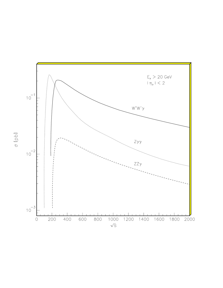
Figure 1: Total SM cross sections for $e^{+}e^{-}\to W^{+}W^{-}\gamma,\;Z^{0}Z^{0}\gamma,\;Z^{0}\gamma\gamma$ (in pb) as a function of $\sqrt{s}$.

Next we study the influence of each of the three anomalous parameters $a_{0},a_{c}$ and $a_{n}$ separately in order to gauge the impact of each on the cross section. Note that $\sigma(W^{+}W^{-}\gamma)$ depends on all three parameters, while $\sigma(Z^{0}Z^{0}\gamma)$ and $\sigma(Z^{0}\gamma\gamma)$ depend only on $a_{0}$ and $a_{c}$. Figure 2 shows the dependence of the three total cross sections of Figure 1 at $\sqrt{s}=500$ GeV on the anomalous parameters. In each case the cross section is normalised to its SM value, and the cuts are the same as in Figure 1.

Figure 2: Influence of the anomalous parameters on the total cross sections, normalised to their SM values, at $\sqrt{s}=500$ GeV.

As expected the dependence on the $a_{i}$ is quadratic, since they appear linearly in the matrix element. The fact that the minimum of the curves is close to the SM point $a_{i}=0$ shows that the interference between the anomalous and standard parts of the matrix element is small. The anomalous parameters have a markedly different effect on the three cross sections. Evidently $a_{0}$ has the largest influence, particularly on $\sigma(Z^{0}Z^{0}\gamma)$. The reason for this is easily understood. The anomalous process $e^{+}e^{-}\to\gamma^{*}\to Z^{0}Z^{0}\gamma$ has a much larger impact on $\sigma(Z^{0}Z^{0}\gamma)$ since there are only six other SM diagrams. In contrast, $e^{+}e^{-}\to\gamma^{*}\to W^{+}W^{-}\gamma$ has a much larger SM ‘background’ set of diagrams to contend with. Note also that the anomalous contributions are enhanced by a factor $1/\cos^{4}\theta_{w}$ compared to the $WW\gamma\gamma$ vertex.

Of course the important question is which of the three processes offers the best chance of detecting an anomalous quartic coupling at a given collider energy. To answer this we need to combine the information from Figs. 1 and 2 to see whether enhanced sensitivity can overcome a smaller overall event rate. We also need to consider correlations between different anomalous contributions to the same cross section.

We consider two experimental scenarios: unpolarised $e^{+}e^{-}$ collisions at $200$ GeV with $\int{\cal L}=150$ pb^-1, and at $500$ GeV with ${\cal L}=300$ fb${}^{-1}/\,$year. Starting with the $W^{+}W^{-}\gamma$ process, Figure 3 shows the contours in the $(a_{i},a_{j})$ plane that correspond to $+2,+3\,\sigma$ deviations from the SM cross section at $\sqrt{s}=200$ GeV. Note that there are three ellipses, one for each combination of the three anomalous couplings. Evidently the sensitivity to $a_{0}$ and $a_{n}$ is comparable, corresponding to $a_{i}<{\cal O}(100)$ for this luminosity. The corresponding limit on $a_{c}$ is some three to four times larger. Figure 4 shows the same contours but now at $500$ GeV. The dramatic improvement in sensitivity (now $a_{i}<{\cal O}(1)$) comes partly from the higher collision energy (which allows for more energetic photons) but mainly from the much higher luminosity. A correlation between the effects of $a_{0}$ and $a_{c}$ (solid ellipses) is noticeable at this energy.

Figure 3: Contour plots for $+2,+3\,\sigma$ deviations from the SM $e^{+}e^{-}\to W^{+}W^{-}\gamma$ total cross section at $\sqrt{s}=200$ GeV with $\int{\cal L}=150$ pb^-1, when two of the three anomalous couplings are non-zero.

Figure 4: As for Figure 3, but for $\sqrt{s}=500$ GeV with $\int{\cal L}=300$ fb^-1.

We have already anticipated a significant improvement in sensitivity for this process when the beams are polarised. Specifically, with right-handed electrons (and left-handed positrons) we suppress a large number of SM ‘background’ diagrams where the $W^{\pm}$ are attached to the fermion line. The effect of 100$\%$ beam polarisation of this type is shown in Figure 5. Assuming the same luminosity we obtain a factor of approximately 3 improvement in the sensitivity to an individual anomalous coupling.

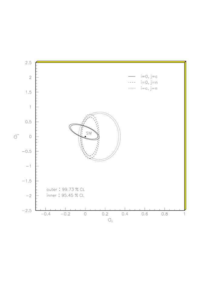
Figure 5: As for Figure 4, but with 100% beam polarisation.

Turning to the sensitivity of the $Z^{0}Z^{0}\gamma$ and $Z^{0}\gamma\gamma$ processes, Figure 6 shows the sensitivity of the latter to $a_{0}$ and $a_{c}$ at $\sqrt{s}=200$ GeV with $\int{\cal L}=150$ pb^-1 and unpolarised beams. For comparison, we also show the corresponding $W^{+}W^{-}\gamma$ contours from Figure 3. The $Z^{0}\gamma\gamma$ process gives a significant improvement in sensitivity, particularly for $a_{c}$. Since the SM cross sections at this energy are comparable (see Figure 1), the improvement comes mainly from the enhanced sensitivity of the matrix element to the anomalous couplings in the $Z^{0}\gamma\gamma$ case.

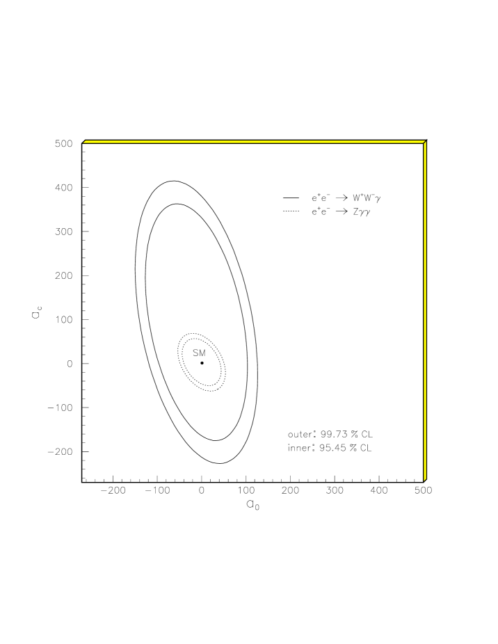
Figure 6: Contour plots for $+2,+3\,\sigma$ deviations from the SM $e^{+}e^{-}\to Z^{0}\gamma\gamma$ total cross section at $\sqrt{s}=200$ GeV with $\int{\cal L}=150$ pb^-1. For comparison, the corresponding contours for the $e^{+}e^{-}\to W^{+}W^{-}\gamma$ process from Figure 3 are also shown.

Finally, Figure 7 compares the sensitivity of all three processes to $a_{0}$ and $a_{c}$ at $\sqrt{s}=500$ GeV with $\int{\cal L}=300$ fb^-1 and unpolarised beams. The best sensitivity is now provided by the $Z^{0}Z^{0}\gamma$ process (particularly for $a_{c}$), despite the fact that it has the smallest cross section of all the three processes. Note that polarising the beams has little effect on the sensitivity of the $Z^{0}Z^{0}\gamma$ and $Z^{0}\gamma\gamma$ processes to the anomalous couplings, since the left-handed and right-handed couplings of the $Z^{0}$ to the electron are similar.

Figure 7: As for Figure 6, but for $\sqrt{s}=500$ GeV with $\int{\cal L}=300$ fb^-1 and including also the $e^{+}e^{-}\to Z^{0}Z^{0}\gamma$ process.

4 Discussion and Conclusions

We have investigated the sensitivity of the processes $e^{+}e^{-}\to W^{+}W^{-}\gamma,\,Z^{0}Z^{0}\gamma$ and $Z^{0}\gamma\gamma$ to genuine anomalous quartic couplings $(a_{0},a_{c},a_{n})$ at the canonical centre-of-mass energies $\sqrt{s}=200$ GeV (LEP2) and $500$ GeV (LC). Key features in determining the sensitivity for a given process and collision energy, apart from the fundamental process dynamics, are the available photon energy $E_{\gamma}$, the ratio of anomalous diagrams to SM ‘background’ diagrams, and the polarisation state of the weak bosons [4].

At $\sqrt{s}=200$ GeV the process $e^{+}e^{-}\to Z^{0}\gamma\gamma$ leads to the tightest bounds on the contour of $(a_{0},a_{c})$, while the process $e^{+}e^{-}\to W^{+}W^{-}\gamma$ is needed to set bounds also on $a_{n}$. Note that the contours of $(a_{0},a_{n})$ and $(a_{c},a_{n})$ can then be improved using the knowledge of the tighter bounds on the contour of $(a_{0},a_{c})$ from $Z^{0}\gamma\gamma$ production. At this energy $Z^{0}\gamma\gamma$ benefits kinematically from producing only one massive boson, which leaves more energy for the photons as well as having fewer ‘background’ diagrams. On the other hand $W^{+}W^{-}\gamma$ production at this energy suffers from the lack of phase space available for energetic photon emission, although this is partially compensated by the production of longitudinal bosons, which gives rise to higher sensitivity to the anomalous couplings.

At $\sqrt{s}=500$ GeV, the effects mentioned above conspire in a somewhat different way. All three processes are now well above their threshold, and hence the availability of phase space for energetic photons is less of an issue. The importance of the longitudinal polarisation of the massive bosons increases and even though the same number of diagrams contributes to $Z^{0}Z^{0}\gamma$ production as to $Z^{0}\gamma\gamma$ production, far tighter bounds on the anomalous couplings can be expected from the former process. The production of longitudinally polarised bosons is comparable in the $W^{+}W^{-}\gamma$ and $Z^{0}Z^{0}\gamma$ processes, but the higher signal to background ratio for the latter leads to a better sensitivity to $a_{0}$ and $a_{c}$.

The ability to polarise the beams leads to a significant improvement in the sensitivity of the $W^{+}W^{-}\gamma$ process, since about a third of the contributing diagrams are removed. With polarised beams the tightest bounds now come from this process. The sensitivity of the $e^{+}e^{-}\to Z^{0}Z^{0}\gamma$ process is hardly affected by beam polarisation. Furthermore, for the typical (large) luminosities expected at future linear colliders [9] the magnitude of the total cross section itself plays a less important role.

The $500$ GeV comparison emphasises the importance of the longitudinal polarisation states of the massive bosons ($Z^{0}Z^{0}\gamma$ and $Z^{0}\gamma\gamma$ are more or less comparable otherwise). This suggests that the $e^{+}e^{-}\to W^{+}W^{-}Z^{0}$ process should be more sensitive to anomalous couplings than $e^{+}e^{-}\to W^{+}W^{-}\gamma$, since all three final-state particles can be longitudinal polarised. With the expected linear collider luminosity, the somewhat smaller cross section should not be an issue, and the ratio of background to signal diagrams is the same as for $W^{+}W^{-}\gamma$ production. Unfortunately this process is only sensitive to $a_{n}$. Furthermore, since there is no photon in the final state 4-dimensional operators can also contribute to anomalous couplings (i.e. an anomalous $W^{+}W^{-}Z^{0}Z^{0}$ vertex) and the analysis becomes significantly more complicated.

Finally it is important to emphasise that in our study we have only considered ‘genuine’ quartic couplings from new six-dimensional operators. We have assumed that all other anomalous couplings are zero, including the trilinear ones. Since the number of possible couplings and correlations is so large, it is in practice very difficult to do a combined analysis of all couplings simultaneously. In fact, it is not too difficult to think of new physics scenarios in which effects are only manifest in the quartic interactions. One example would be a very heavy excited W resonance produced and decaying as in $W^{+}\gamma\to W^{*}\to W^{+}\gamma$.

In principle, any non-zero trilinear coupling could affect the limits obtained on the quartic couplings. For example, in equation (4) we showed explicitly how a non-zero trilinear coupling ($\lambda$) can generate an anomalous $WW\gamma\gamma$ quartic interaction to compete with the ‘genuine’ ones that we have considered. The (dimensionless) strength of the former is $eg\lambda$, while for the latter it is $e^{2}a_{i}\langle E_{ext.}\rangle\langle E_{int.}\rangle/\Lambda^{2}$, where $E_{ext.}$ and $E_{int.}$ are the typical energy scales of the photons entering the vertex. (Here we are considering, as a specific example, the $e^{+}e^{-}\to W^{+}W^{-}\gamma$ process.) Since $\Lambda=M_{W}$, $\langle E_{ext.}\rangle\sim 25$ GeV and $E_{int.}\sim[5\sqrt{s}+4(\sqrt{s}-\langle E_{ext.}\rangle)]/9\sim 190$ GeV , both for $\sqrt{s}=200$ GeV, we see immediately that the relative contributions of the two types of couplings are in the approximate ratio $3\lambda:a_{i}$. Now, at LEP2 upper limits on trilinear couplings like $\lambda$ are already ${\cal O}(0.1)$ [2]. In contrast, we have shown that the limits achievable on the $a_{i}$ are ${\cal O}(100)$. Hence we already know that the anomalous trilinear couplings have a minimal impact on our analysis. The same argument holds at higher collider energies. The limits on the trilinear couplings will always be so much smaller than those on the quartic couplings, that they can safely be ignored in studies of the latter.

Acknowledgements
This work was supported in part by the EU Fourth Framework Programme ‘Training and Mobility of Researchers’, Network ‘Quantum Chromodynamics and the Deep Structure of Elementary Particles’, contract FMRX-CT98-0194 (DG 12 - MIHT). AW gratefully acknowledges financial support in the form of a ‘DAAD Doktorandenstipendium im Rahmen des gemeinsamen Hochschulprogramms III für Bund und Länder’.

References

-
[1]
K. Hagiwara, R.D. Peccei, D. Zeppenfeld and K. Hikasa,
Nucl. Phys. B282 (1987) 253.
Triple Gauge Boson Couplings, G. Gounaris et al., in ‘Physics at LEP2’, Vol. 1, p. 525-576, CERN (1995) [hep-ph/9601233]. -
[2]
ALEPH Collaboration: R. Barate et al., Phys. Lett. B422 (1998) 369;
preprint CERN-EP-98-178, November 1998 [hep-ex/9901030].
OPAL Collaboration: G. Abbiendi et al., preprint CERN-EP-98-167, October 1998 [hep-ex/9811028]. - [3] S. Godfrey, Quartic Gauge Boson Couplings, Proc. International Symposium on Vector Boson Self-Interactions, UCLA, February 1995.
- [4] G. Blanger and F. Boudjema, Phys. Lett. B288 (1992) 201.
- [5] G. Abu-Leil and W.J. Stirling, J. Phys. G21 (1995) 517.
- [6] O.J.P. boli, M.C. Gonzalz-Graca and S.F. Novaes, Nucl. Phys. B411 (1994) 381.
- [7] V. Barger et al., Phys. Rev. D39 (1989) 146.
- [8] T. Stelzer and W.F. Long, Comput. Phys. Commun. 81 (1994) 357.
- [9] B.H. Wiik, The TESLA Project, Lecture at the Ettore Majorana school ‘From the Planck Length to the Hubble Radius’, Erice, Sept. 98, to appear in the proceedings.