ITEP-TH-10/99
KANAZAWA 99-03

Infrared Behaviour of the Gauge Boson Propagator in a Confining Theory

M.N. Chernodub^a, M.I. Polikarpov^a and V.I. Zakharov^b
a Institute of Theoretical and Experimental Physics,

B.Cheremushkinskaya 25, Moscow, 117259, Russia

and

^b Max-Planck Institut für Physics, Werner-Heisenberg Institut,
80805 Munich, Germany.

We study the gauge boson propagator in the dual Abelian Higgs theory which confines electric charges. The confinement is due to dual Abrikosov-Nielsen-Olesen strings. We show that the infrared double pole $1/{(p^{2})}^{2}$ in the propagator is absent due to the confinement phenomenon. Instead, specific angular singularities signal the eventual set in of the confinement. These angular singularities are a manifestation of the confining strings.

1. The most popular explanation of the quark confinement is the dual superconductor model of QCD vacuum [1]. There is a lot of numerical facts demonstrating that in the abelian projection [2] of the lattice gluodynamics the monopoles are the relevant infrared degrees of freedom responsible for the quark confinement and for formation of confining string (see, $e.g.$, reviews [3] and references therein).

There exists yet another, so to say “phenomenological” point of view on the quark confinement formulated in terms of the gluon propagator. Namely, one argues [4, 5] that if the gluon propagator has a double pole in the infrared region then the quark–anti–quark potential gets a linear attractive contribution at large distances and this implies the quark confinement. On the other hand, Gribov and Zwanziger  [6] argued that elimination of the gauge copies leads to a counter-intuitive vanishing of the gluon propagator in the infrared region. Some analytical studies [7] confirm this behaviour, while the others [8] predict a singular gluon propagator in the infrared limit. Recent numerical simulations in lattice gluodynamics [9] show that the gluon propagator seems to vanish at small momenta. However, the systematic errors due to a finite lattice size do not allow to reach a final conclusion.

In this paper we study analytically the infrared behaviour of the gauge boson propagator in a $U(1)$ theory with confinement. Namely we consider the dual Abelian Higgs theory in which magnetic monopoles are condensed and electric charges are confined. The motivation is that this theory can be considered as an effective infrared theory of $SU(2)$ gluodynamics [10]. Moreover, it was found recently that the vacuum of the lattice $SU(2)$ gluodynamics is well described by the dual Abelian Higgs model in which monopoles play the role of the Higgs particles [11]. We define an analogue of the gluon propagator in terms of abelian variables and show that the infrared double pole in the propagator is absent in the confining phase of the model. We do not observe the vanishing of the gluon propagator in the infrared region  [6] either. In the case considered, the confinement properties of the theory are rather manifested through string like singularities of the propagator. Since the dual Abelian Higgs model imitates QCD in the infrared region a similar behaviour might be exhibited by the gluon propagator in QCD, at least in the gauges considered.

2. To evaluate the propagator we utilize the Zwanziger local field theory of electrically and magnetically charged particles [12]. The theory contains two vectors potentials, namely the gauge field $A_{\mu}(x)$ and the dual gauge field $B_{\mu}(x)$, which interact covariantly with electric and magnetic currents, respectively. The corresponding Lagrangian is:

$${\cal L}={\cal L}_{Zw}(A,B)+i\,e\,j^{e}_{\mu}(x)\,A_{\mu}(x)+i\,g\,j^{m}_{\mu}(x)\,B_{\mu}(x)\,,$$ (1)

where $e$ ($g$) stands for the electric (magnetic) charge, and $j^{e}_{\mu}$ ($j^{e}_{\mu}$) is the electric (magnetic) external current. The Zwanziger Lagrangian ${\cal L}_{Zw}$ is given by the following equation [12]:

$${\cal L}_{Zw}(A,B) = \frac{1}{2}(n\cdot[\partial\wedge A])^{2}+\frac{i}{2}(n\cdot[\partial\wedge A])(n\cdot{[\partial\wedge B]}^{d})$$ (2)

$$+\frac{1}{2}(n\cdot[\partial\wedge B])^{2}-\frac{i}{2}(n\cdot[\partial\wedge B])(n\cdot{[\partial\wedge A]}^{d})\}\,,$$

where we have used the standard notations:

$$[A\wedge B]_{\mu\nu}=A_{\mu}B_{\nu}-A_{\nu}B_{\mu}\,,\quad(n\cdot[A\wedge B])_{\mu}=n_{\nu}(A\wedge B)_{\nu\mu}\,,\quad{(G)}^{d}_{\mu\nu}=\frac{1}{2}\varepsilon_{\mu\nu\lambda\rho}G_{\lambda\rho}\,.$$ (3)

Despite the theory (1) apparently contains two gauge fields, $A_{\mu}$ and $B_{\mu}$, there is only one physical particle (a massless photon) in the spectrum [12, 13]. The Lagrangian (1) depends on an arbitrary constant unit vector $n_{\mu}$, $n^{2}_{\mu}=1$, while physical observables are insensitive to the direction of $n$ provided the Dirac quantization condition, $e\cdot g=2\pi m$, $m\in{Z\!\!\!Z}$, is satisfied [12].

3. Within the dual superconductor approach [1] a pure $SU(2)$ gauge theory is regarded as a theory of dynamical abelian monopoles which are required to be condensed in the color confining phase. According to eq.(1) the theory of monopoles interacting with an external electric source $j^{e}$ (quark current) is described by the following partition function [10]:

$${\cal Z}[j^{e}] = \int{\cal D}A{\cal D}B{\cal D}\Phi\,\exp\Bigl{\{}-\int\mbox{d}^{4}x\Bigl{(}{\cal L}_{Zw}(A,B)+\frac{1}{2}{|(\partial_{\mu}+igB_{\mu})\Phi|}^{2}$$ (4)

$$+\lambda{({|\Phi|}^{2}-\eta^{2})}^{2}-iej^{e}_{\mu}A_{\mu}\Bigr{)}\Bigr{\}}\,.$$

Here $\Phi$ is the field of condensed monopoles, the constants $\lambda,\eta^{2}$ are positive and we choose to work in the Euclidean space. In this approach, the abelian field $A_{\mu}$ corresponds to the diagonal component $A^{3}_{\mu}$ of the $SU(2)$ gauge field $A^{a}_{\mu}$ in a certain abelian gauge. According to the abelian dominance phenomenon [14] the field $A_{\mu}$ is responsible for the infrared properties of the theory. For the sake of simplicity we consider below the London limit, $\lambda\to\infty$. The final results remain however qualitatively unchanged if we relax the condition on the coupling $\lambda$.

The spectrum of the model (4) contains a string–like topological excitation which carries a quantized electric flux. This string is the dual analogue of the Abrikosov–Nielsen–Olesen (ANO) string [15] in the Abelian Higgs model. Stretched between quarks and anti-quarks the string leads to the color confinement. The confinement phenomenon exists in the theory already at the classical level, the linear string contribution to the quark potential is dominant at large distances [10, 16, 17] and survives at small quark–anti-quark separations [18].

4. The gauge field propagator is defined as:

$$D_{\mu\nu}(x,y)\equiv<A_{\mu}(x)A_{\nu}(y)>=-\frac{1}{e^{2}}\,\frac{\delta^{2}}{\delta j^{e}_{\mu}(x)\,\delta j^{e}_{\nu}(y)}\frac{{\cal Z}[j^{e}]}{{\cal Z}[0]}{\Biggl{|}}_{j^{e}=0}\,,$$ (5)

and is an analogue of the gluon propagator in gluodynamics.

To specify the propagator completely we choose the axial gauge $n_{\mu}A_{\mu}=0$ in expressions (4,5). Moreover, using the methods of Refs. [19] we obtain readily a string representation for ${\cal Z}[j^{e}]$:

$${\cal Z}[j^{e}]\propto\oint\limits_{\partial\Sigma=0}{\cal D}\Sigma\,\exp\Bigl{\{}-\int\mbox{d}^{4}x\int\mbox{d}^{4}y\Bigl{[}\frac{2\pi^{2}}{e^{2}}j^{2}_{\mu}(x)D_{M_{B}}(x-y)\cdot X_{\mu\nu}j^{e}_{\nu}(y)$$

$$+4\eta^{2}\pi^{2}j^{e}_{\mu}(x)D_{M_{B}}(x-y)\cdot{(\partial\cdot n)}^{-1}n_{\nu}\Sigma_{\mu\nu}(y)+\eta^{2}\pi^{2}\Sigma_{\mu\nu}(x)D_{M_{B}}(x-y)\Sigma_{\mu\nu}(y)\Bigr{]}\Bigr{\}}\,,$$ (6)

where $D_{M_{B}}$ is the propagator of a massive scalar field $(-\partial^{2}_{\mu}+M^{2}_{B})D_{M_{B}}(x)=\delta^{(4)}(x)$, $M_{B}=e\eta$ is the mass of the dual gauge boson $B_{\mu}$, and the integration in eq.(6) is performed over all closed world sheets of the ANO strings (see Refs. [19]). Moreover, $X_{\mu\nu}$ is a differential operator which in the momentum representation has the form:

$$X_{\mu\nu}(p) = \delta_{\mu\nu}-\frac{1}{(p\cdot n)}(p_{\mu}n_{\nu}+p_{\nu}n_{\mu})+\frac{p_{\mu}p_{\nu}}{{(p\cdot n)}^{2}}+\frac{M^{2}_{B}}{{(p\cdot n)}^{2}}(\delta_{\mu\nu}-n_{\mu}n_{\nu})\,.$$ (7)

Substituting (6) in (5) we get the following expression for the propagator:

$$D^{\mathrm{axial}}_{\mu\nu}(p) = \frac{1}{p^{2}+M^{2}_{B}}\cdot X_{\mu\nu}(p)+D^{\mathrm{str}}_{\mu\nu}(p)\,,$$ (8)

$$D^{\mathrm{str}}_{\mu\nu}(p) = -\frac{\eta^{4}e^{2}}{p^{2}+M^{2}_{B}}\cdot\frac{1}{(p\cdot n)}\cdot\int\frac{\mbox{d}^{4}k}{{(2\pi)}^{2}}\frac{1}{k^{2}+M^{2}_{B}}\frac{n_{\alpha}n_{\beta}}{(k\cdot n)}\cdot{<\Sigma_{\mu\alpha}(p)\Sigma_{\nu\beta}(-k)>}_{\Sigma}\,,$$ (9)

Note that the expression (8) for the gluon propagator is exact in the London limit (there are no loop contributions to eq.(8))!

The first term in the propagator is already known from Ref. [13] while the second term describes interaction of the gauge boson with the ANO strings. Moreover the string–string correlation function in (9) is defined as:

$${<{{\cal O}}>}_{\Sigma} = \frac{1}{{\cal Z}^{\mathrm{str}}}\,\oint\limits_{\partial\Sigma=0}{\cal D}\Sigma\,e^{-S_{\mathrm{str}}(\Sigma)}\,{\cal O}\,,\quad{\cal Z}_{\mathrm{str}}=\oint\limits_{\partial\Sigma=0}{\cal D}\Sigma\,e^{-S_{\mathrm{str}}(\Sigma)}\,,$$ (10)

$$S_{\mathrm{str}}(\Sigma) = \pi^{2}\eta^{2}\int\mbox{d}^{4}x\int\mbox{d}^{4}y\,\Sigma_{\mu\nu}(x)D_{M_{B}}(x-y)\Sigma_{\mu\nu}(y)\,.$$ (11)

The expression (11) is the action for the ANO strings in the Abelian Higgs model in the London limit [19].

An exact expression for the string–string correlator is unknown. Taking into account the closeness condition, $\partial_{\mu}\Sigma_{\mu\nu}(x)=0$, one can parametrize this correlator as follows:

$${<\Sigma_{\mu\alpha}(x)\Sigma_{\nu\beta}(y)>}_{\Sigma}=\varepsilon_{\mu\alpha\xi\rho}\,\varepsilon_{\nu\beta\zeta\rho}\,\partial_{\xi}\partial_{\zeta}\,{{\tilde{D}}}^{\Sigma}\Bigl{(}{(x-y)}^{2}\Bigr{)}\,,$$ (12)

or, in the momentum representation:

$${<\Sigma_{\mu\alpha}(k)\Sigma_{\nu\beta}(-p)>}_{\Sigma} = {(2\pi e)}^{2}\delta(k-p)\cdot\varepsilon_{\mu\alpha\xi\rho}\,\varepsilon_{\nu\beta\zeta\rho}\,p_{\xi}p_{\zeta}\,{{D}}^{\Sigma}(p^{2})\,,$$ (13)

where ${{D}}^{\Sigma}(p^{2})={{D}}^{\Sigma}(p^{2};e,\eta)$ is a scalar function, which is related to the function ${{\tilde{D}}}^{\Sigma}$ in eq.(12) via the Fourier transform.

Substituting the string correlation function (13) into eq. (9) we get:

$$D^{\mathrm{str}}_{\mu\nu}(p) = \frac{M_{B}^{4}}{{(p^{2}+M^{2}_{B})}^{2}}\,D^{\Sigma}(p^{2})\,\Bigl{[}\Bigl{(}\delta_{\mu\nu}-\frac{p_{\mu}n_{\nu}+p_{\nu}n_{\mu}}{{(p\cdot n)}}+\frac{p_{\mu}p_{\nu}}{{(p\cdot n)}^{2}}\Bigr{)}$$ (14)

$$-\frac{p^{2}}{{(p\cdot n)}^{2}}\cdot(\delta_{\mu\nu}-n_{\mu}n_{\nu})\Bigr{]}\,.$$

Thus, the gluon propagator (8) in the axial gauge has the form:

$$D^{\mathrm{axial}}_{\mu\nu}(p) = \frac{1}{p^{2}+M^{2}_{B}}\,\Bigl{[}\Bigl{(}\delta_{\mu\nu}+\frac{p_{\mu}n_{\nu}+p_{\nu}n_{\mu}}{{(p\cdot n)}}-\frac{p_{\mu}p_{\nu}}{{(p\cdot n)}^{2}}\Bigr{)}\cdot\Bigl{(}1+\frac{M^{4}_{B}D^{\Sigma}(p^{2})}{p^{2}+M^{2}_{B}}\Bigr{)}$$ (15)

$$+\frac{1}{{(p\cdot n)}^{2}}\cdot(\delta_{\mu\nu}-n_{\mu}n_{\nu})\cdot M^{2}_{B}\,\Bigl{(}1-M^{2}_{B}\frac{p^{2}\,D^{\Sigma}(p^{2})}{p^{2}+M^{2}_{B}}\Bigr{)}\Bigr{]}\,.$$

The propagator has singularities not only in the $p^{2}$ plane but in the variable $(p\cdot n)$ as well. Which is not unusual of course because $n_{\mu}$-dependence enters through the gauge fixing. What is unusual, however, is that the singular in $(p\cdot n)$ terms appear not only in the longitudinal structures but in front of $(\delta_{\mu\nu}-n_{\mu}n_{\nu})$ as well. While the former singularities do not contribute to the physical amplitudes and can be removed by changing the gauge, the same is not true in the latter case. The singular factors in front of the $(\delta_{\mu\nu}-n_{\mu}n_{\nu})$ structure appear due to the Dirac strings which are present in the Zwanziger Lagrangian (2). The issue of these singularities is finally settled through observation that the relation between physical observables and the propagator becomes more subtle than, say, in QED (see Ref. [17]). Here we are concerned primarily with formal properties of the propagator itself.

A general parametrization of the gauge boson propagator in the axial gauge is  [5]:

$$D^{\mathrm{axial}}_{\mu\nu}=\Bigl{(}\delta_{\mu\nu}+\frac{p_{\mu}n_{\nu}+p_{\mu}n_{\nu}}{{(p\cdot n)}}-\frac{p_{\mu}p_{\nu}}{{(p\cdot n)}^{2}}\Bigr{)}\cdot F(p^{2})-\frac{1}{{(p\cdot n)}^{2}}\cdot(\delta_{\mu\nu}-n_{\mu}n_{\nu})\cdot G(p^{2})\,,$$ (16)

where $F(p^{2})$ and $G(p^{2})$ are the coefficient functions which characterize the vacuum of the theory. A comparison of eq. (15) with eq. (16) gives the following relation between these coefficient functions and the string correlation function $D^{\Sigma}$ introduced above:

$$F(p^{2}) = \frac{1}{p^{2}+M^{2}_{B}}\,\Bigl{(}1+\frac{M^{4}_{B}D^{\Sigma}(p^{2})}{p^{2}+M^{2}_{B}}\Bigr{)}\,;$$ (17)

$$G(p^{2}) = -\frac{M^{2}_{B}}{p^{2}+M^{2}_{B}}\cdot\Bigl{(}1-M^{2}_{B}\frac{p^{2}\,D^{\Sigma}(p^{2})}{p^{2}+M^{2}_{B}}\Bigr{)}\,.$$ (18)

Note that the expressions (17) and (18) are non–perturbative even without taking into account the string contributions. Indeed, removing for a moment the string contributions from these relations we get:

$$F^{\mathrm{no-string}}(p^{2})=\frac{1}{p^{2}+M^{2}_{B}}\,,\quad G^{\mathrm{no-string}}(p^{2})=-\frac{M^{2}_{B}}{p^{2}+M^{2}_{B}}\,,$$ (19)

while for the perturbative vacuum one has [5]:

$$F^{\mathrm{pert}}(p^{2})=\frac{1}{p^{2}}\,,\quad G^{\mathrm{pert}}(p^{2})=0\,.$$ (20)

Equations (19) account for the same graphs as in the standard Higgs mechanism, i.e. for insertions of the scalar field condensate.

5. Although the expression (15) for the gluon propagator is exact, it contains an unknown function $D^{\Sigma}(p^{2})$. The infrared behaviour of this function however can be qualitatively understood on physical grounds. Indeed, consider the string part (9) of the gluon propagator (8). This part corresponds to the process, schematically shown in Figure 1: the quark emits a gauge boson $A$ which transforms to a dual gauge boson $B$ via coupling $<A\cdot B>$ which exists in the Zwanziger Lagrangian (2). The dual gauge boson transforms back to the gauge boson after scattering on a closed ANO string world sheet $\Sigma$. The intermediate string state is described by the function $D^{\Sigma}(p^{2})$ and this state can be considered as a glueball state with the photon quantum numbers $1^{-}$.

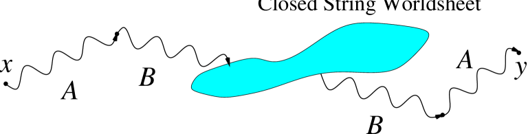
Figure 1: String contribution (9) to gluon propagator (8).

The behaviour of the function $D^{\Sigma}(p^{2})$ in the infrared region, $p\to 0$, can be estimated as follows:

$$D^{\Sigma}(p^{2})=\frac{C}{p^{2}+M_{\mathrm{gl}}^{2}}+\dots\,,$$ (21)

where $C$ is a dimensionless parameter and $M_{\mathrm{gl}}$ is the mass of the lowest $1^{-}$ glueball. The dots denote the contributions of heavier states. Thus, according to eqs. (21,17,18) the coefficient functions $F$ and $G$ in the infrared limit, $p\to 0$, become:

$$\begin{array}[]{ccl}F^{\mathrm{infr}}(p^{2})&=&\frac{1}{M^{2}_{B}}+\frac{C}{M^{2}_{\mathrm{gl}}}+O(p^{2})\,,\\ G^{\mathrm{infr}}(p^{2})&=&-1+O(p^{2})\,,\end{array}$$ (24)

Note that neither double, $1/{(p^{2})}^{2}$, nor ordinary, $1/p^{2}$, pole are exhibited by the gluon propagator (16,24) in the infrared limit. There are gauge dependent $1/(p\cdot n)$ singularities which reflect the presence of Dirac strings. Therefore our gauge boson propagator does not vanish in the infrared limit either. In view of this, the vanishing of the propagator at $p\to 0$ predicted in [6] seems to be specific for the special gauge choice in QCD which leads to a nontrivial Fundamental Modular Region.

Our demonstration of non-existence of the double pole in the propagator is based on the infrared behaviour (21) of the string–string correlation function $D^{\Sigma}$. Suppose for a moment that our prescription for $D^{\Sigma}$ is not correct and the double pole exists in the propagator. We would conclude then from eq. (17) that the string correlation function has a double pole at $p^{2}=0$. It would imply, in turn, long range correlations of the string world sheets and, as a result, the absence of the mass gap and quark confinement! Indeed, if the strings are long-range correlated then the quarks associated with the string ends would also be long–range propagating objects. Thus, the absence of a double pole in the gluon propagator is a direct consequence of confinement, at least in the dual superconductor model of infrared QCD considered here.

It is worth emphasizing that our qualitative results do not depend on the gauge choice. While up to now we discussed the axial gauge, $n_{\mu}A_{\mu}=0$, the choice of the Landau gauge, $\partial_{\mu}A_{\mu}=0$, leads to a mere shift of the operator (7) which enters the definition of the propagator (8):

$$X^{\mathrm{Landau}}_{\mu\nu}(p)=X_{\mu\nu}(p)+\frac{p^{2}+M^{2}_{B}}{p^{2}\,(p\cdot n)}(p_{\mu}n_{\nu}+p_{\nu}n_{\mu})-\frac{p^{2}+M^{2}_{B}}{(p^{2})^{2}\,(p\cdot n)^{2}}((p\cdot n)^{2}+p^{2})\cdot p_{\mu}p_{\nu}\,.$$

Due to this shift an ordinary pole $1/p^{2}$ appears in a longitudinal term which is irrelevant, however, for gauge-invariant observables.

To summarize, the gauge boson propagator in the model considered does not display either a double pole in $p^{2}$ or vanishing in the limit $p^{2}\to 0$, the phenomena thought to be a signature for the quark confinement [5, 6]. It is rather the stringy singularities in the $(p\cdot n)$ variable which signal the confinement. The other closest infrared singularities present in the gauge boson propagator correspond to the mass of the gauge boson and the lowest $1^{-}$ glueball mass. Moreover in our case the confining potential is not related to the infrared behaviour of the gauge boson propagator in the conventional way: $\tilde{V}(r)=\int\,e^{ipr}D_{00}(p)\mbox{d}^{3}p$. Indeed, $D_{00}$ contains $1/(p\cdot n)$ singularities (see eq.(15)) related to the Dirac string, and thus $\tilde{V}(r)$ is gauge dependent. The right way to obtain the gauge independent expression for the potential $V(r)$ is to evaluate the expectation value of the Wilson loop for the field $A_{\mu}$ in the string representation of the model. In the string representation the $1/(p\cdot n)$ singularities in the propagator play the crucial role: they transform into the confining ANO strings. The details of this calculation are given in Ref.[17].

6. M.N.Ch. and M.I.P. feel much obliged for the kind hospitality extended to them at the Max-Planck-Institute for Physics in Munich where this work has been started. M.I.P wishes to express his gratitude to the members of the Department of Physics of the Kanazawa University where this work has been completed. This work was partially supported by the grants INTAS-96-370, INTAS-RFBR-95-0681, RFBR-96-02-17230a and RFBR-96-15-96740. The work of M.N.Ch. was supported by the INTAS Grant 96-0457 within the research program of the International Center for Fundamental Physics in Moscow. M.I.P. was supported by JSPS (Japan Society for the Promotion of Science) Fellowship Program.

References

-
[1]
G. ’t Hooft, ”High Energy Physics”,
Ed. by A. Zichichi, Editrice Compositori, Bolognia, 1976;
S. Mandelstam, Phys. Rept. 23C (1976) 245. - [2] G. ’t Hooft, Nucl. Phys. B190 (1981) 455.
-
[3]
T. Suzuki, Nucl. Phys. B (Proc. Suppl.) 30
(1993) 176;
M.I. Polikarpov, Nucl. Phys. B (Proc. Suppl.) 53 (1997) 134;
M.N. Chernodub and M.I. Polikarpov, in ”Confinement, Duality and Non-perturbative Aspects of QCD”, p.387, Ed. by Pierre van Baal, Plenum Press, 1998; hep-th/9710205;
G.S. Bali, preprint HUB-EP-98-57, Jan. 1998, hep-ph/9809351. - [4] G.B. West, Phys. Lett. 115B (1982) 468.
- [5] M. Baker, J.S. Ball and F. Zachariasen, Phys. Rev. D37 (1988) 1036; Erratum-ibid. D37 (1988) 3785.
-
[6]
V.N. Gribov, Nucl. Phys. B139 (1978) 1;
D. Zwanziger, Nucl. Phys. B364 (1991) 127. -
[7]
U. Häbel et al., Z.Phys. A 336 (1990) 423;
L. von Smekal, A. Hauck and R. Alkofer, Phys. Rev. Lett. 79 (1997) 3591; Ann. Phys. 267 (1998) 1;
D. Atkinson and J.C.R. Bloch, Mod. Phys. Lett A13 (1998) 1055. -
[8]
M. Baker, J.S. Ball and F. Zachariasen, Nucl.
Phys. B186 (1981) 531;
N. Brown and M.R. Pennington, Phys. Rev. D39 (1989) 2723;
A.I. Alekseev, Phys. Lett. B344 (1995) 325;
F.T. Hawes, P. Maris, C.D. Roberts, Phys. Lett. B440 (1998) 353. -
[9]
C. Bernard, C. Parrinello and A. Soni, Phys. Rev.
D49 (1994) 1585;
H. Nakajima and S. Furui, hep-lat/9809081, hep-lat/9809078;
A. Cucchieri, Phys. Lett. B422 (1998) 233;
D. B. Leinweber et al.; preprint ADP-98-72/T339, hep-lat/9811027;
J.P. Ma, preprint AS-ITP-99-07 hep-lat/9903009. - [10] S. Maedan and T. Suzuki, Prog. Theor. Phys. 81 (1989) 229.
-
[11]
S. Kato, S. Kitahara, N. Nakamura and T. Suzuki,
Nucl. Phys. B520 (1998) 323;
M.N. Chernodub et al., preprint KANAZAWA-98-19, hep-lat/9902013. -
[12]
D. Zwanziger, Phys. Rev. D3 (1971) 343;
R.A. Brandt, F. Neri, and D. Zwanziger, Phys. Rev. D19 (1979) 1153;
M. Blagoević and Senjanović, Phys. Rep. 157 (1988) 233. -
[13]
A.P. Balachandran, H. Rupertsberger, and J. Schechter,
Phys. Rev. D11 (1975) 2260;
T. Suzuki, Prog. Theor. Phys. 81 (1989) 752. -
[14]
Z.F. Ezawa and A. Iwazaki,
Phys.Rev. D25 (1982) 2681;
T. Suzuki and I. Yotsuyanagi, Phys. Rev., D42 (1990) 4257;
G.S. Bali et. al., Phys. Rev. D54 (1996) 2863. -
[15]
A.A. Abrikosov, JETP 32 (1957) 1442;
H.B. Nielsen and P. Olesen, Nucl. Phys. B61 (1973) 45. -
[16]
H. Suganuma, S. Sasaki and H. Toki, Nucl. Phys.
B435 (1995) 207;
S. Sasaki, H. Suganuma and H. Toki, Phys.Lett. B387 (1996) 145. - [17] F.V. Gubarev, M.I. Polikarpov and V.I. Zakharov, Phys. Lett. B438 (1998) 147.
-
[18]
F.V. Gubarev, M.I. Polikarpov and
V.I. Zakharov, preprint ITEP-TH-73-98,
hep-th/9812030. -
[19]
P. Orland, Nucl. Phys. B428, (1994) 221;
M. Sato and S. Yahikozawa, Nucl. Phys. B436 (1995) 100;
E.T. Akhmedov et al., Phys. Rev. D53 (1996) 2087;
M.I. Polikarpov, U.-J. Wiese and M.A. Zubkov, Phys. Lett., 309B (1993) 133.