1. The interest in the interplay between hard inclusive and exclusive reactions has recently been revived by theoretical work on deeply virtual Compton scattering (DVCS) and skewed parton distributions (SPDs) [1]. These SPDs are hybrid objects, which combine properties of form factors and of ordinary parton distributions. In fact, reduction formulas reveal the close connection of these quantities. It has also been shown recently [2, 3] that at moderately large momentum transfer real and virtual Compton scattering off protons approximately factorises into a hard parton-photon subprocess and a soft proton matrix element described by new form factors specific to Compton scattering. These new form factors, as the ordinary electromagnetic ones, represent moments of SPDs and can be modelled by overlaps of light-cone wave functions [2, 3], which provide the link between exclusive and inclusive reactions. In this overlap representation, which implies Feynman’s end-point mechanism, the SPDs are given as products of ordinary parton distributions and exponentials of $t\,(1-x)/x$, provided one makes a simplifying assumption about the wave functions. Here $t$ is the squared momentum transfer experienced by the proton, and $x$ the usual fraction of the light-cone plus component of the proton momentum carried by the active parton, i.e. the one entering the parton-photon subprocess.

It is to be emphasised that the soft physics mechanism is complementary to the perturbative one [4], and that both contributions have to be taken into account. We argue, however, that for large angle Compton scattering the soft contribution, although formally representing a power correction to the asymptotically leading perturbative one, dominates at experimentally accessible momentum transfers. For electromagnetic nucleon form factors it has been shown that agreement with the data can be achieved by calculating both hard scattering and soft overlap contributions with a moderately asymmetric wave function, and the soft contribution was indeed found to dominate for $-t$ of order $10~{}{\rm GeV}^{2}$ [5]. The soft contribution to large angle Compton scattering, evaluated with the same wave function, is also in reasonable agreement with available data [3]. The perturbative contribution has been calculated in [6, 7] to leading twist accuracy and is way below the Compton data unless strongly asymmetric, i.e. end-point concentrated distribution amplitudes are used. These give however results dominated by contributions from the soft end-point regions, where the assumptions of a leading twist perturbative calculation break down, and have also been criticised on other grounds, cf. for instance [5, 8]. From the results of [5, 6] we estimate that the perturbative contribution to Compton scattering amounts to less than $10\%$ of the data for $-t$ in the region of a few $10~{}{\rm GeV}^{2}$.

The data of many exclusive observables exhibit approximate dimensional counting rule behaviour, a fact that is frequently considered as evidence for the dominance of perturbative physics. In our opinion, this conclusion is unjustified: The running of $\alpha_{\rm s}$ and the evolution of the hadronic wave functions often provide large powers of $\ln{s}$, which should modify the dimensional counting rule behaviour substantially. Such modifications are however not seen in the data. In these reactions the effective scale of hardness is typically rather low, so that the effect of the logarithms should be especially strong. One may argue that the effective scale in these cases is so small that the running coupling becomes frozen. This indicates, however, that one is not in the perturbative regime (the freezing of $\alpha_{\rm s}$ being certainly a nonperturbative effect), and also means that power corrections can be large. In the soft physics approach, on the other hand, approximate dimensional counting rule behaviour holds in a limited range of momentum transfer, which is controlled by the transverse size of the hadrons involved. For electromagnetic form factors and Compton scattering this mimicked scaling behaviour is well in agreement with experiment [2, 3, 5]. Naturally the question arises how to interpret the approximate dimensional counting rule behaviour in other exclusive reactions, such as proton-proton elastic scattering. A tentative answer to this question will be given in this article.

The main purpose of this paper is however to present a phenomenological study of real and virtual Compton scattering in the soft physics approach in order to facilitate comparison with other theoretical results on this reaction and with future experimental data that might be obtained at Jefferson Lab or at an ELFE-type accelerator at DESY or CERN.

2. Let us briefly outline the calculation of large angle Compton scattering in the soft physics approach; for details we refer to [3]. The amplitude is evaluated from the handbag diagram shown in Fig. 1. The large blobs denote soft proton wave functions, i.e. wave functions with their perturbative tails removed, and the small blob attached to the photon lines represents the elementary subprocess, Compton scattering off quarks or antiquarks, which is calculated in lowest order QED with point-like quark-photon couplings. The physical situation is that of a hard photon-parton scattering and the soft emission and reabsorption of a parton by the hadron, as in the familiar handbag diagram for DVCS or inclusive deeply inelastic scattering (DIS).

    

Figure 1: The handbag diagram for Compton scattering off protons. The horizontal lines represent any number of spectator partons.

Four-momenta are also defined in Fig. 1. As usual we define the Mandelstam variables $s=(p+q)^{2}$, $t=\Delta^{2}$, $u=(p-q^{\prime})^{2}$, and write $Q^{2}=-q^{2}$ for the incoming photon virtuality and $m$ for the proton mass. We require $s$, $-u$ and $-t$ to be large on a hadronic scale, which defines large angle scattering and the region of validity of our calculation.

We assume that soft hadron wave functions are dominated by parton virtualities in the range $|k_{i}^{2}|\raisebox{-4.0pt}{$\,\stackrel{{\scriptstyle\textstyle<}}{{\sim}}\,$}\Lambda^{2}$, where $\Lambda$ is a hadronic scale in the GeV region, and by intrinsic transverse parton momenta ${\bf k}_{\perp}{}_{i}$ (defined with the respect to their parent hadron’s momentum) that satisfy ${\bf k}_{\perp i}^{2}/x_{i}^{\phantom{.}}\raisebox{-4.0pt}{$\,\stackrel{{\scriptstyle\textstyle<}}{{\sim}}\,$}\Lambda^{2}$. This leads to an approximate equality of the Mandelstam variables in the parton-photon subprocess and the overall proton-photon reaction up to corrections of order $\Lambda^{2}\,(1-Q^{2}/t)$. Therefore the parton-photon scattering is hard, and when calculating it we approximate the momenta $k_{j}^{\phantom{.}}$, $k^{\prime}_{j}$ of the active partons as being on shell, collinear with their parent hadrons and with light cone fractions $x_{j}^{\phantom{.}}=x^{\prime}_{j}=1$.

Under the above assumptions the helicity amplitudes ${\cal M}_{\mu^{\prime}\nu^{\prime},\,\mu\nu}$ for large angle Compton scattering can be written in terms of soft proton matrix elements and hard parton-photon scattering amplitudes ${\cal H}_{\mu^{\prime}\lambda^{\prime},\,\mu\lambda}$. We define proton and photon helicities in the photon-proton c.m., which is convenient for phenomenological applications and comparison with other results. The amplitudes conserving the proton helicity are explicitly given by

$${\cal M}_{\mu^{\prime}+,\,\mu+}=\;2\pi\alpha_{\rm em}\left[{\cal H}_{\mu^{\prime}+,\,\mu+}\,(R_{V}+R_{A})\,+\,{\cal H}_{\mu^{\prime}-,\,\mu-}\,(R_{V}-R_{A})\right]\,,$$ (1)

proton helicity flip will be discussed shortly. $\mu$ and $\mu^{\prime}$ are the helicities of the incoming and outgoing photon, and $\nu,\,\lambda$ and $\nu^{\prime},\,\lambda^{\prime}$ those of the incoming and outgoing proton and parton, respectively. From parity invariance one has ${\cal M}_{\mu^{\prime}\nu,\,\mu\nu}=(-1)^{\mu^{\prime}-\mu}{\cal M}_{-\mu^{\prime}-\nu,\,-\mu-\nu}$ and an analogous equation for ${\cal H}_{\mu^{\prime}\lambda,\,\mu\lambda}$. For the sake of legibility we label explicit helicities only by their signs, i.e. in the matrix elements we write $+$, $-$ instead of $+1/2$, $-1/2$ for fermions.

Since the partons are taken as massless there is no parton helicity flip in the photon-parton subprocess amplitudes, which read

$${\cal H}_{++,\,++} = 2\,\sqrt{\frac{s}{-u}}\>\frac{s+Q^{2}}{s}\,,\hskip 30.00005pt{\cal H}_{-+,\,-+}\>=\>2\,\sqrt{\frac{-u}{s}}\>\frac{s}{s+Q^{2}}\,,$$

$${\cal H}_{-+,\,++} = 2\,\frac{Q^{2}}{s+Q^{2}}\>\frac{t}{\sqrt{-su}}\,,\hskip 27.0pt{\cal H}_{-+,\,0+}\>=\>-2\>\frac{Q}{s+Q^{2}}\>\sqrt{-2t}\,,$$ (2)

and ${\cal H}_{++,\,-+}\,=\,{\cal H}_{++,\,0+}\,=\,0.$ Within the accuracy of our calculation the subprocess amplitudes are real; $\alpha_{\rm s}$-corrections, however, will lead to non-zero imaginary parts.

The soft proton matrix elements in Eq. (1), $R_{V}$ and $R_{A}$, represent form factors specific to Compton scattering [2, 3]. $R_{V}$ is defined by

$$\sum_{a}e_{a}^{2}\,\int_{0}^{1}\,\frac{{\rm{d}}x}{x}\,p^{+}\int{{\rm{d}}z^{-}\over 2\pi}\,e^{i\,xp^{+}z^{-}}\langle p^{\prime},\nu^{\prime}|\,\overline{\psi}{}_{a}(0)\,\gamma^{+}\,\psi_{a}(z^{-})-\overline{\psi}{}_{a}(z^{-})\,\gamma^{+}\,\psi_{a}(0)\,|p,\nu\rangle$$ (3)

$$\hskip 80.00012pt=R_{V}(t)\,\bar{u}(p^{\prime},\nu^{\prime})\,\gamma^{+}u(p,\nu)\,+R_{T}(t)\,\frac{i}{2m}\bar{u}(p^{\prime},\nu^{\prime})\sigma^{+\rho}\Delta_{\rho}u(p,\nu)\,,$$

where the sum runs over quark flavours $a$ ($u$, $d$, …), $e_{a}$ being the electric charge of quark $a$ in units of the positron charge. The matrix element is to be evaluated in a frame where the light-cone plus momentum of the proton is unchanged, i.e. where $\Delta^{+}=0$. There is an analogous equation for the axial vector proton matrix element, which defines the form factor $R_{A}$. Note that, as in DIS and DVCS, only the plus components of the proton matrix elements enter in the Compton amplitude, which is a nontrivial dynamical feature given that, in contrast to DIS and DVCS, not only the plus components of the proton momenta but also their minus and transverse components are large now. Due to time reversal invariance the form factors $R_{V}$, $R_{A}$ etc. are real functions. As the definition (3) reveals they are $1/x$ moments of SPDs at zero skewedness parameter $\zeta=-\Delta^{+}/p^{+}$ [1].

Some remarks on the proton spin are in order. The description of $R_{T}$ or of its electromagnetic counterpart $F_{2}$ involves components in the proton wave function, where the parton helicities do not add up to the helicity of the hadron, whose modelisation is beyond the scope of this work. It is however natural to assume that $R_{T}/R_{V}\sim F_{2}/F_{1}$, and the latter ratio is known to be $F_{2}/F_{1}\simeq-m^{2}/t$ at large $t$. Terms going with $R_{T}$ in proton helicity non-flip amplitudes are then corrections of order $m^{2}/t$ and have been omitted in Eq. (1), given that already our evaluation of the handbag diagrams is only accurate up to corrections in $\Lambda^{2}/t$. For proton helicity flip we obtain amplitudes going with $R_{T}{\sqrt{-t/m^{2}}}$ and $R_{V,A}{\sqrt{-m^{2}/t}}$, which are down compared with non-flip amplitudes by a factor of ${\sqrt{-m^{2}/t}}$. Within our accuracy observables involving unpolarised and longitudinally polarised protons can thus be calculated from the proton helicity non-flip amplitudes (1) alone.

3. Before we present numerical results for the observables of real and virtual Compton scattering we have to model the new form factors. In a frame where $\Delta^{+}=0$ the form factors $R_{V}$ and $R_{A}$ can be represented by overlaps of light-cone wave functions summed over all Fock states, in close analogy with the famous Drell-Yan formula [9] for the electromagnetic form factor:

$$R_{V,A}(t)=\sum_{N,\beta,j}\,\kappa_{V,A}^{\phantom{.}}\,e^{2}_{j}\,\int\,[{\rm{d}}x]_{N}[{\rm{d}}^{2}{\bf k}_{\perp}]_{N}\,\frac{1}{x_{j}}\,\Psi^{*}_{N\beta}(x_{i}^{\phantom{.}},{\bf k}^{\prime}_{\perp i})\,\Psi_{N\beta}(x_{i},{\bf k}_{\perp}{}_{i})$$ (4)

with $\kappa_{V}=1$ and $\kappa_{A}=2\lambda_{j}$. Each Fock state $N$ is described by a number of terms, each with its own momentum space wave function $\Psi_{N\beta}$, where $\beta$ labels different spin-flavour combinations of the partons. The sum over the active parton, $j$, with charge $e_{j}$ and helicity $\lambda_{j}$ runs over all partons in a given Fock state. Primed and unprimed intrinsic transverse momenta are related to each other by ${\bf k}^{\prime}_{\perp i}={\bf k}_{\perp}{}_{i}\,-\,x_{i}\,{\bf\Delta}_{\perp}$ for $i\neq j$ and ${\bf k}^{\prime}_{\perp j}={\bf k}_{\perp}{}_{j}\,+\,(1-x_{j})\,{\bf\Delta}_{\perp}$, and $[{\rm d}x]_{N}[{\rm d}^{2}{\bf k}_{\perp}]_{N}$ is the $N$-particle integration measure, cf. [3]. Assuming a simple Gaussian ${\bf k}_{\perp}{}_{i}$-dependence of the soft Fock state wave functions,

$$\Psi_{N\beta}(x_{i},{\bf k}_{\perp}{}_{i})\propto\exp\left[-a_{N}^{2}\sum_{i=1}^{N}\frac{{\bf k}_{\perp i}^{2}}{x_{i}}\right]\,,$$ (5)

one can explicitly carry out the momentum integrations in (4). The ansatz (5) satisfies various theoretical requirements [10, 11] and is in line with our hypothesis that the soft hadronic wave functions are dominated by transverse momenta with ${\bf k}_{\perp i}^{2}/x_{i}^{\phantom{.}}\raisebox{-4.0pt}{$\,\stackrel{{\scriptstyle\textstyle<}}{{\sim}}\,$}\Lambda^{2}$, necessary to achieve the factorisation of the Compton amplitudes into soft and hard parts. The results of the transverse momentum integrations for $R_{V}$ and $R_{A}$ are respectively related with the Fock state contributions to the unpolarised and polarised parton distribution functions. For simplicity one may further assume a common transverse size parameter $a_{N}=\hat{a}$ for all Fock states. This immediately allows one to sum over them, without specifying the $x_{i}$-dependence of the wave functions. One then arrives at

$$R_{V}(t)=\sum_{a}\,e_{a}^{2}\,\int\frac{{\rm{d}}x}{x}\,\exp{\left[\frac{1}{2}\hat{a}^{2}t\frac{1-x}{x}\right]}\;\{q_{a}(x)+\bar{q}_{a}(x)\}\,,$$ (6)

and the analogue for $R_{A}$ with $q_{a}+\bar{q}_{a}$ replaced by $\Delta q_{a}+\Delta\bar{q}_{a}$. The result (6) is very instructive as it elucidates the link between the parton distributions of DIS and exclusive reactions. Evaluating the form factors from the parton distributions of GRV [12] and with $\hat{a}=1~{}{\rm GeV}^{-1}$, one already finds results for the Compton cross section in fair agreement with experiment. In order to improve on the approximation (6) the lowest three Fock states were modelled explicitly in [3], assuming specific distributions amplitudes and fitting the wave function parameters to the GRV parton distributions at $x>0.5$. In the present letter we make use of the model form factors as given there.

These form factors behave as $1/t^{2}$ in the momentum transfer range from about 5 to 15 GeV² and, consequently, the Compton cross section shows approximate $s^{-6}$ scaling behaviour for photon energies in the region of several GeV, cf. [3]. With increasing $-t$ the form factors gradually turn into the soft physics asymptotics $\propto 1/t^{4}$, which follows from the $x_{i}$-dependence of the model wave functions at the end points. In that region of $t$ the perturbative contribution will take the lead.

4. The contribution of virtual Compton scattering to the unpolarised $ep\to ep\gamma$ cross section can be decomposed into four partial cross sections (for details see [13]): the cross sections for transverse photons (reducing to the unpolarised cross section for real Compton scattering, i.e. for $Q^{2}=0$) and for longitudinal photons,

$$\frac{{\rm{d}}\sigma_{\rm T}}{{\rm{d}}t} = \frac{1}{32\pi s(s+Q^{2})}\;\sum_{\mu^{\prime},\nu^{\prime},\nu}\;|{\cal M}_{\mu^{\prime}\nu^{\prime},\,+\nu}|^{2}\,,$$

$$\frac{{\rm{d}}\sigma_{\rm L}}{{\rm{d}}t} = \frac{1}{32\pi s(s+Q^{2})}\;\sum_{\mu^{\prime},\nu^{\prime},\nu}\;|{\cal M}_{\mu^{\prime}\nu^{\prime},\,0\,\nu}|^{2}\,,$$ (7)

and the transverse-transverse and longitudinal-transverse interference terms

$$\frac{{\rm{d}}\sigma_{\rm TT}}{{\rm{d}}t} = -\frac{1}{64\pi s(s+Q^{2})}\;{\rm Re}\,\sum_{\mu^{\prime},\nu^{\prime},\nu}\;{\cal M}_{\mu^{\prime}\nu^{\prime},\,+\nu}^{\ast}\,{\cal M}_{\mu^{\prime}\nu^{\prime},\,-\nu}^{\phantom{\ast}}\,,$$

$$\frac{{\rm{d}}\sigma_{\rm LT}}{{\rm{d}}t} = -\frac{\sqrt{2}}{64\pi s(s+Q^{2})}\;{\rm Re}\,\sum_{\mu^{\prime},\nu^{\prime},\nu}\;{\cal M}_{\mu^{\prime}\nu^{\prime},\,0\,\nu}^{\ast}\,[{\cal M}_{\mu^{\prime}\nu^{\prime},\,+\nu}^{\phantom{\ast}}-{\cal M}_{\mu^{\prime}\nu^{\prime},\,-\nu}^{\phantom{\ast}}]\,.$$ (8)

In certain kinematical regions, namely for small values of $-t/Q^{2}$ or of the ratio $\varepsilon$ of longitudinal and transverse photon flux in the Compton process, the full $ep\to ep\gamma$ cross section receives substantial contributions from the Bethe-Heitler process, where the final state photon is radiated by the electron. This process is completely calculable for values of $t$ where the elastic proton form factors $F_{1}$ and $F_{2}$ are known, and in suitable kinematics its interference with the Compton process can be used to study the latter at amplitude level.

For real Compton scattering a number of polarisation observables have been introduced [14]. Of particular interest is the initial state helicity correlation

$$A_{\rm LL}\,\frac{{\rm{d}}\sigma}{{\rm{d}}t}\>=\>\frac{1}{2}\,\left[\frac{{\rm{d}}\sigma(++)}{{\rm{d}}t}-\frac{{\rm{d}}\sigma(+-)}{{\rm{d}}t}\right]\>=\>\frac{1}{32\pi s^{2}}\,\sum_{\mu^{\prime},\nu^{\prime}}\;\left[|{\cal M}_{\mu^{\prime}\nu^{\prime},\,++}|^{2}-|{\cal M}_{\mu^{\prime}\nu^{\prime},\,+-}|^{2}\right]\,,$$ (9)

which , when $R_{T}$ and mass corrections are neglected, measures the product $R_{V}R_{A}$, while the unpolarised cross section receives contributions from $R_{V}^{2}$ and $R_{A}^{2}$ only:

$$\frac{{\rm{d}}\sigma}{{\rm{d}}t} = \frac{2\pi\alpha_{\rm em}^{2}}{s^{2}}\,\left[\,\frac{1}{2}(R_{V}^{2}+R_{A}^{2})\left(-\frac{s}{u}-\frac{u}{s}\right)+(R_{V}^{2}-R_{A}^{2})\,\right]\,,$$

$$A_{\rm LL}\,\frac{{\rm{d}}\sigma}{{\rm{d}}t} = \frac{2\pi\alpha_{\rm em}^{2}}{s^{2}}\;R_{V}R_{A}\left(\frac{u}{s}-\frac{s}{u}\right)\,.$$ (10)

Other spin observables for real Compton scattering are the incoming photon asymmetry $\Sigma$ and the helicity transfer parameter $D_{\rm LL}$,

$$\Sigma\,\frac{{\rm{d}}\sigma}{{\rm{d}}t}\>=\>\frac{1}{2}\,\left[\frac{{\rm{d}}\sigma_{\perp}}{{\rm{d}}t}-\frac{{\rm{d}}\sigma_{\parallel}}{{\rm{d}}t}\right]\>=\>\frac{1}{32\pi s^{2}}\;{\rm Re}\,\sum_{\mu^{\prime},\nu^{\prime},\nu}\;{\cal M}_{\mu^{\prime}\nu^{\prime},\,+\nu}^{\ast}\,{\cal M}_{\mu^{\prime}\nu^{\prime},\,-\nu}^{\phantom{\ast}}\,,$$

$$D_{\rm LL}\,\frac{{\rm{d}}\sigma}{{\rm{d}}t}\>=\>\frac{{\rm{d}}\sigma(+,+)}{{\rm{d}}t}-\frac{{\rm{d}}\sigma(+,-)}{{\rm{d}}t}\>=\>\frac{1}{32\pi s^{2}}\,\sum_{\nu^{\prime},\nu}\;\left[|{\cal M}_{+\nu^{\prime},\,+\nu}|^{2}-|{\cal M}_{+\nu^{\prime},\,-\nu}|^{2}\right]\,$$ (11)

where $\perp$ and $\parallel$ respectively refer to linear photon polarisation normal to and in the scattering plane. For real Compton scattering the photon helicity turns out to be strictly conserved in the soft physics approach (up to possible $\alpha_{\rm s}$ corrections), cf. Eq. (2), so that $\Sigma$ and $D_{\rm LL}$ acquire the values 0 and $1$, respectively. In the diquark model, a variant of the standard perturbative Brodsky-Lepage approach to exclusive reactions [4], small deviations from these values have been obtained [15] since the photon helicity flip amplitudes are non-zero, although suppressed by powers of $1/s$ in this model. The leading twist hard scattering results of [7] deviate only slightly from our soft physics values.

Making use of the numerical results for $R_{V}$ and $R_{A}$ given in [3] (cf. Sect. 3) we evaluate the initial state helicity correlation $A_{\rm LL}$ (9) for real Compton scattering. Its $\cos{\theta}$-dependence (cf. Fig. 2) is roughly given by $(s^{2}-u^{2})/(s^{2}+u^{2})$, and reflects that of the corresponding helicity correlation for the photon-parton subprocess. It is opposite in sign to the diquark model predictions [15]. In the leading twist hard scattering approach the two available results [6, 7] strongly differ from each other and from the result presented here.

Figure 2: Predictions for the initial state helicity correlation $A_{\rm LL}$ at photon energies of 4 GeV (long-dashed) and 12 GeV (solid line) in the proton rest frame vs. $\cos{\theta}$, where $\theta$ is the c.m. scattering angle. The short-dashed line represents the contribution from the valence Fock state alone at 12 GeV. $A_{\rm LL}$ is evaluated with the Compton form factors calculated in [3].

Predictions for the various cross sections for virtual Compton scattering are shown in Fig. 3 at a photon energy of 5 GeV in the proton rest frame and for a set of $Q^{2}$ values. Comparing with the only other available results, namely those from the diquark model [13], we see that the transverse cross section in both approaches comes out rather similar, while the other three cross sections are generally larger and with a smoother $Q^{2}$-dependence in the soft physics approach than in the diquark model. In contrast to the diquark model the transverse-transverse interference term is strictly zero now in the limit $Q^{2}=0$, where the ratio ${\rm{d}}\sigma_{\rm TT}/{\rm{d}}\sigma_{\rm T}$ is equivalent to the photon asymmetry $\Sigma$ defined in Eq. (11). We note that in the soft physics approach ${\rm{d}}\sigma_{\rm LT}/{\rm{d}}\sigma_{\rm T}\leq 0$ as long as $R_{V}^{2}\geq R_{A}^{2}$, which is satisfied with our representation (6) in terms of parton distributions.

Figure 3: Predictions for the virtual Compton cross sections at $s=10$ GeV² and different values of $Q^{2}$ vs. $\cos{\theta}$.

Fig. 4 shows the difference between the full $ep\to ep\gamma$ cross section and the contribution of the Compton process alone, divided by the full cross section. As expected the Bethe-Heitler process becomes dominant for increasing $\cos{\theta}$, i.e. for decreasing $-t$. For the kinematics considered here the relative importance of Bethe-Heitler and Compton is similar to the one found in the diquark model [13]. A detailed investigation of the interplay between the Bethe-Heitler and Compton contributions and their interference as a function of the various kinematical variables is beyond the scope of this letter.

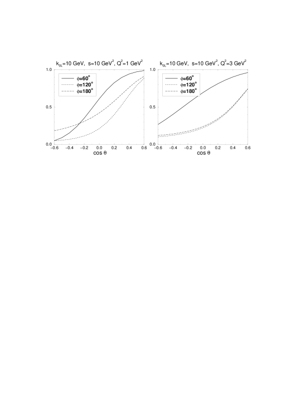
Figure 4: The difference between the full $ep\to ep\gamma$ cross section and the contribution of the Compton process alone, divided by the full cross section, as a function of $\cos{\theta}$ at fixed $k_{0L}$, $s$, $Q^{2}$ and $\phi$. The azimuthal angle $\phi$ between the electron and hadron planes is defined in [13], and $k_{0L}$ denotes the electron beam energy in the proton rest frame.

In Ref. [13] the relevance of the beam asymmetry for $ep\to ep\gamma$

$$A_{\rm L}=\frac{{\rm{d}}\sigma(+)-{\rm{d}}\sigma(-)}{{\rm{d}}\sigma(+)+{\rm{d}}\sigma(-)}\,,$$ (12)

where the labels $+$ and $-$ denote the lepton beam helicity, has been pointed out. It is sensitive to the imaginary part of the longitudinal-transverse interference in the Compton process, while ${\rm{d}}\sigma_{\rm LT}/{\rm{d}}t$ measures its real part. In the diquark model [13] the virtual Compton contribution to $A_{\rm L}$ is very small but the full asymmetry is spectacularly enhanced in regions of strong interference between the Compton and the Bethe-Heitler amplitudes. In these regions $A_{\rm L}$ essentially measures the relative phase between the complex virtual Compton amplitudes and the real Bethe-Heitler ones. In the standard perturbative approach a non-zero value of $A_{\rm L}$ is also to be expected in the interference region because of the perturbatively generated phases of the Compton amplitudes. In the soft physics approach, on the other hand, $A_{\rm L}$ is zero since all amplitudes are real within the accuracy of our calculation. Due to $\alpha_{\rm s}$-corrections in the photon-parton subprocess $A_{\rm L}$ may become non-zero in the soft physics approach.

One may finally consider the transverse polarisation (normal to the scattering plane) of the initial or the final state proton. As is well known the corresponding polarisation asymmetry requires both non-vanishing proton helicity flip amplitudes and relative phases between flip and non-flip amplitudes. In the soft physics mechanism all amplitudes are approximately real. Moreover, as we argued above, the helicity flip amplitudes are suppressed compared to the non-flip ones by a factor ${\sqrt{-m^{2}/t}}$. We therefore predict very small proton polarisations in the soft physics approach. Because of hadron helicity conservation the transverse proton spin asymmetries are zero in the standard perturbative approach [7]. Only the diquark model provides both necessary ingredients and predicts proton polarisations of up to $10\%$ [15].

5. To summarise, the detailed predictions for real and virtual Compton scattering obtained from the handbag diagram exhibit interesting features and characteristic helicity dependences. Comparison with perturbative calculations, either obtained within the standard hard scattering approach or its diquark variant, reveals marked differences which may allow one to distinguish between these mechanisms experimentally. Data for these observables from Jefferson Lab or other accelerators are eagerly awaited.

It is particularly interesting that the soft physics approach can account for the experimentally observed approximate dimensional counting rule behaviour, at least for Compton scattering and for form factors. This tells us that it is premature to infer the dominance of perturbative physics from the observed scaling behaviour . One may object that the perturbative explanation (leaving aside the logarithms from the running of $\alpha_{\rm s}$ and from the evolution) works for many exclusive reactions, while in the soft physics approach the approximate counting rule behaviour is accidental, depending on specific properties of a given reaction. In our opinion, and we are going to substantiate this briefly, the approximate counting rule behaviour is an unavoidable feature of the soft physics approach. Let us consider proton-proton elastic scattering at $s,\;-t,\;-u\gg\Lambda^{2}$. Viewing this process as in Fig. 5 we recognise the factorisation into soft hadron matrix elements and a hard scattering of spin 1/2 partons. This model for hadron-hadron scattering bears resemblance to the parton scattering model invented long time ago [16]. The hard scattering kernels are dimensionless and therefore depend only on the ratio $t/s$ and on the parton helicities. The soft hadron matrix elements represent form factors similar to the electromagnetic or the Compton form factors, except that the parton charges do not appear.

 

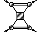
Figure 5: The soft physics mechanism for $pp$ elastic scattering. The horizontal lines represent any number of spectator partons.

All these form factors are smooth functions of the momentum transfer and, when scaled by $t^{2}$, exhibit a broad maximum in the $-t$-range from about 5 to 15 GeV², set by the transverse hadron size, i.e. by a scale of order 1 GeV^-1. To see how the maximum can be at $-t$ quite above a GeV² consider for example the form factor $R_{V}(t)$ as given in (6). For the position of the maximum of $t^{2}R_{V}(t)$ we obtain

$$-t=4\hat{a}^{-2}\,\left\langle{\frac{1-x}{x}}\right\rangle^{-1}$$ (13)

where the $t$-dependent mean value $\langle\frac{1-x}{x}\rangle$ is defined by weighting with the integrand of (6). It comes out around $0.5$ at the value of $t$ where the maximum is taken. Note also that both sides of the implicit equation (13) increase with $-t$. It is thus approximately satisfied over a certain $t$-range, in other words the maximum of the scaled form factor is quite broad.

Without a full-fledged analysis, i.e. without specifying the hard scattering kernels ${\cal H}(t/s)$, it is clear now that the soft physics approach provides approximate $s^{-10}$ scaling of ${\rm{d}}\sigma/{\rm{d}}t$ in proton-proton scattering at large, fixed scattering angle and $s$ in the range from $10~{}{\rm GeV}^{2}$ to $30~{}{\rm GeV}^{2}$. The agreement of this prediction with experiment [17] is reasonable as we checked. We remind however the reader that the proton-proton data show fluctuations superimposed to the $s^{-10}$ behaviour. These fluctuations, if a real dynamical feature, tell us that there still is another momentum scale relevant in that kinematical region, contradicting the very idea of dimensional scaling.

For mesons all our arguments apply in a similar fashion. The corresponding form factors approximately behave like $1/t$ over a certain range of $t$, again mimicking dimensional counting. This leads to a scaling prediction of $s^{-8}$ for fixed angle meson-proton scattering.

Acknowledgements: This work has been partially funded through the European TMR Contract No. FMRX-CT96-0008. T.F. is supported by Deutsche Forschungsgemeinschaft. P.K. thanks DESY Zeuthen for support and the hospitality extended to him.

References

-
[1]
D. Müller, D. Robaschik, B. Geyer, F.-M. Dittes
and J. Hořejši,
Fortschr. Physik 42, 101 (1994),
hep-ph/9812448;
X. Ji, Phys. Rev. Lett. 78, 610 (1997); Phys. Rev. D55, 7114 (1997);
A.V. Radyushkin, Phys. Rev. D56, 5524 (1997). - [2] A.V. Radyushkin, Phys. Rev. D58, 114008 (1998).
-
[3]
M. Diehl, T. Feldmann, R. Jakob and P. Kroll,
hep-ph/9811253,
Eur. Phys. J. C,
DOI 10.1007/s100529901100. - [4] G.P. Lepage and S.J. Brodsky, Phys. Rev. D22, 2157 (1980).
- [5] J. Bolz and P. Kroll, Z. Phys. A356, 327 (1996).
- [6] M. Vanderhaeghen, P.A.M. Guichon and J. Van de Wiele, Nucl. Phys. A622, 144c (1997).
- [7] A. Kronfeld and B. Nižić, Phys. Rev. D44, 3445 (1991); Erratum Phys. Rev. D46, 2272 (1992).
-
[8]
N. Isgur and C.H. Llewellyn Smith,
Nucl. Phys. B317, 526 (1989);
A.V. Radyushkin, Nucl. Phys. A532, 141c (1991). - [9] S.D. Drell and T.-M. Yan, Phys. Rev. Lett. 24, 181 (1970).
- [10] B. Chibisov and A.R. Zhitnitsky, Phys. Rev. D52, 5273 (1995).
- [11] S.J. Brodsky, hep-ph/9807212.
- [12] M. Glück, E. Reya and A. Vogt, Z. Phys. C67, 433 (1995); Eur. Phys. J. C5, 461 (1998); M. Glück, E. Reya, M. Stratmann and W. Vogelsang, Phys. Rev. D53, 4775 (1996).
- [13] P. Kroll, M. Schürmann and P.A.M. Guichon, Nucl. Phys. A598, 435 (1996).
- [14] H. Rollnik and P. Stichel, in: Elementary Particle Physics, Springer Tracts in Mod. Phys., Vol. 79 (Springer, Berlin 1976).
- [15] P. Kroll, M. Schürmann and W. Schweiger, Intern. J. Mod. Phys. A6, 4107 (1991).
-
[16]
H.D.I. Abarbanel, S.D. Drell and F.J. Gilman,
Phys. Rev. 177, 2458 (1969);
D. Cline, F. Halzen and M. Waldrop, Nucl. Phys. B55, 157 (1973);
D. Horn and M. Moshe, Nucl. Phys. B48, 557 (1972); ibid. B57, 139 (1973). - [17] C.W. Akerlof et al., Phys. Rev. 159, 1138 (1967).