INT #DOE/ER/40561-37-INT98
Low-Energy Parity-Violation and New Physics

Abstract

The new physics sensitivity of a variety of low-energy parity-violating (PV) observables is analyzed. A comparison is made between atomic PV for a single isotope, atomic PV using isotope ratios, and PV electron-hadron and electron-electron scattering. The complementarity among these observables, as well as with high-energy processes, is emphasized. Theoretical uncertainties entering the interpretation of low-energy measurements are discussed.

I Introduction

Low-energy parity-violating (PV) observables have played an important role in uncovering the structure of the electroweak sector of the Standard Model. Now that the predictions of the Standard Model have been tested and confirmed at the one-loop level over a wide range of processes and energies [1], attention has turned to the search for physics beyond the Standard Model. In this regard, low-energy parity-violation continues to provide important information. As has been noted by several authors[2, 3, 4], the recent precise determination of the cesium weak charge, ${Q_{\scriptscriptstyle W}}$, in an atomic parity-violation (APV) experiment performed by the Boulder group[5] places stringent constraints on a variety of new physics scenarios. The importance of this benchmark measurement is reflected, in part, by the efforts of other experimental groups to determine ${Q_{\scriptscriptstyle W}}$ for cesium as well as other atoms[6, 7, 8]. Future improvements in the APV sensitivity to new physics poses a challenge to both atomic experimentalists and theorists. Indeed, given the experimental precision reported by the Boulder group, atomic theory error now constitutes the dominant uncertainty associated with the intepretation of atomic PV (APV) observables. Whether this atomic theory error can be reduced to the level of the experimental uncertainty remains to be seen. An experimental strategy for circumventing the atomic theory uncertainty is to measure PV observables for different atoms along an isotope chain. Standard Model predictions for ratios of such observables are largely atomic theory-independent. Consequently, several groups have undertaken APV isotope ratio measurements in the hopes of minimizing the impact of atomic theory uncertainties on the extraction of new physics constraints[7, 8, 9].

Historically, the use of polarized electrons produced in accelerator experiments has, along with APV, played a part in testing the Standard Model[10, 11, 12]. In the past decade, however, PV electron scattering (PVES) has received less attention than APV in this respect since (a) the experimental precision achievable with APV has improved markedly and (b) interest in PVES has focused on its use in probing the nucleon’s $s\bar{s}$ sea. The interest in nucleon strangeness has spawned a program of experiments at MIT-Bates, Mainz, and the Jefferson Laboratory to measure the left-right asymmetry, ${A_{\scriptscriptstyle LR}}$, on a variety of targets[13, 14, 15]. Recently, the attention of the PVES community has returned to the use of these experiments to probe new physics[16]. In the purely leptonic sector, work on a high-precision PV Möller scattering experiment has begun at SLAC[17]. In addition, a program of “second generation” PVES experiments – designed to look for physics beyond the Standard Model – is under consideration for the Jefferson Lab. The feasibility of such PVES new physics searches stems, in part, from the high luminosity and remarkably stable and clean electron beam achieved by the CEBAF accelerator[18].

Although there have appeared numerous discussions of ${Q_{\scriptscriptstyle W}}($cesium) in the literature recently, relatively little attention has been paid to the other low-energy PV observables mentioned above. In this paper, we therefore consider the new physics sensitivities of APV isotope ratios and PVES asymmetries, making comparison with sensitivities of ${Q_{\scriptscriptstyle W}}$ and high-energy observables. In doing so, we focus on “direct” new physics, that is, extensions of the Standard Model which manifest themselves at low-energies as new four-fermion contact interactions. The sensitivity of APV and PVES to “oblique” new physics has been discussed elsewhere[2, 19, 20, 21, 24]. After quantifying the generic new physics sensitivities of PV observables, we specify to a variety of models in order to illustrate the complementarity of prospective measurements. In particular, we show that to leading order, the elastic $ep$ asymmetry, ${A_{\scriptscriptstyle LR}}(^{1}{\hbox{H}})$ ,and APV isotope ratios, ${\cal R}$, are sensitive to the same combination of possible new interactions. These two observables, while subject to different systematic and theoretical corrections, provide the same window on direct new physics. We also find that a 2-3% determination of ${A_{\scriptscriptstyle LR}}(^{1}{\hbox{H}})$ would improve the new physics reach of low-energy PV by nearly a factor of two over the present cesium APV sensitivity. A similar improvement would obtain if the present cesium atomic theory error were improved by a factor of four. Apart from the Möller asymmetry, the remaining asymmetries display a smaller new physics reach than ${Q_{\scriptscriptstyle W}}$, ${A_{\scriptscriptstyle LR}}(^{1}{\hbox{H}})$ , or ${\cal R}$. In illustrating model variations on the general pattern of new physics sensitivity, we consider additional neutral gauge bosons, leptoquarks, and fermion compositeness. We also discuss the sensitivity of PV observables to R-parity violating supersymmetric interactions and compare this sensitivity with up-dated bounds from super-allowed $\beta$-decay.

The use of low-energy measurements to probe new physics requires that conventional, many-body physics associated with atoms and nuclei be sufficiently well-understood. From this standpoint, we show that, in principle, PVES provides the theoretically “cleanest” new physics probe. This feature is most apparent for PV Möller scattering, as it is a purely leptonic process. In the case of semi-leptonic PV observables, the reason for minimal theoretical uncertainty is two-fold: (a) ${A_{\scriptscriptstyle LR}}$ depends on a ratio of electroweak amplitudes, from which the largest hadronic effects cancel, leaving essentially a dependence on ${Q_{\scriptscriptstyle W}}$ of the target nucleus; and (b) the largest remaining hadronic corrections to this cancellation can be separated from ${Q_{\scriptscriptstyle W}}$ and measured by exploiting their kinematic dependence. Consequently, the dominant uncertainty in the interpretation of PVES new physics studies is likely to be experimental. We illustrate these features in the case of ${A_{\scriptscriptstyle LR}}(^{1}{\hbox{H}})$ and discuss the kinematics to make such a clean separation of ${Q_{\scriptscriptstyle W}}$ feasible.

The situation in the case of APV differs from that of PVES. The atomic theory uncertainty associated with extracting ${Q_{\scriptscriptstyle W}}$ from cesium APV is about four times larger than the experimental error. This situation has prompted the consideration of the isotope ratios ${\cal R}$, from which the dominant atomic theory uncertainties cancel. Unfortunately, ${\cal R}$ carries a problematic sensitivity to changes in the neutron distribution, $\rho_{n}(r)$, from one nucleus to the next along an isotope change. Following on the earlier work of Refs. [25, 26, 27], we analyze the impact which the uncertainties in the neutron distribution, $\rho_{n}(r)$, have on the extraction of new physics limits from ${\cal R}$. We consider several atoms presently under experimental consideration and quantify the level of $\rho_{n}$ uncertainty acceptable in order for relevant new physics limits to be obtained from ${\cal R}$.

Our discussion of these issues is organized as follows. In Section II, we outline our conventions and definitions, and in Section III discuss general new physics sensitivities of low-energy PV observables. In Section IV we illustrate these sensitivities for different new physics scenarios. Section V contains an analysis of theoretical uncertainties. A discussion of kinematic considerations for a prospective PV elastic $ep$ experiment is also included. In Section VI we summarize our conclusions.

II New Physics and the Weak Charge

For each PV observable, the quantity of interest here is the weak charge ${Q_{\scriptscriptstyle W}}$ of the nucleus (electron), which characterizes the strength of the electron axial vector $\times$ nucleus (electron) vector weak neutral current interaction:

$${Q_{\scriptscriptstyle W}}={Q_{\scriptscriptstyle W}^{0}}+\Delta{Q_{\scriptscriptstyle W}}\ \ \ .$$ (1)

Here, ${Q_{\scriptscriptstyle W}^{0}}$ gives the contribution in the Standard Model while $\Delta{Q_{\scriptscriptstyle W}}$ indicates possible contributions from new interactions. We consider ${Q_{\scriptscriptstyle W}}$ to be generated by the low-energy effective Lagrangian

$${\cal L}={\cal L}^{\scriptscriptstyle PV}_{\scriptscriptstyle S.M.}+{\cal L}^{\scriptscriptstyle PV}_{\scriptscriptstyle NEW}\ \ \ ,$$ (2)

where

$${\cal L}^{\scriptscriptstyle PV}_{\scriptscriptstyle S.M.} = {G_{F}\over 2\sqrt{2}}{g_{\scriptscriptstyle A}^{e}}{\bar{e}}\gamma_{\mu}\gamma_{5}e\sum_{f}{g_{\scriptscriptstyle V}^{f}}{\bar{f}}\gamma^{\mu}f$$ (3)

$${\cal L}^{\scriptscriptstyle PV}_{\scriptscriptstyle NEW} = {4\pi\kappa^{2}\over\Lambda^{2}}{\bar{e}}\gamma_{\mu}\gamma_{5}e\sum_{f}{h_{\scriptscriptstyle V}^{f}}{\bar{f}}\gamma^{\mu}f\ \ \ .$$ (4)

Here ${g_{\scriptscriptstyle V}^{f}}=2T_{3}^{f}-4Q_{f}{\sin^{2}\theta_{\scriptscriptstyle W}}$ and ${g_{\scriptscriptstyle A}^{f}}=-2T_{3}^{f}$ are the tree level Standard Model fermion-$Z^{0}$ couplings; ${h_{\scriptscriptstyle V}^{f}}$ characterizes the interaction of the electron axial vector current with the vector current of fermion $f$ for a given extension of the Standard Model; $\Lambda$ is the mass scale associated with the new physics; and $\kappa$ sets the coupling strength. Generally speaking, strongly interacting theories take $\kappa^{2}\sim 1$ while for weakly interacting extensions of the Standard Model one has $\kappa^{2}\sim\alpha$. For scenarios in which the interaction of Eq. (4) is generated by the exchange of a new heavy particle between the electron and fermion, the constant ${h_{\scriptscriptstyle V}^{f}}={\tilde{g}_{\scriptscriptstyle A}^{e}}{\tilde{g}_{\scriptscriptstyle V}^{f}}$, where ${\tilde{g}_{\scriptscriptstyle A}^{e}}$ (${\tilde{g}_{\scriptscriptstyle V}^{f}}$) are the heavy particle axial vector (vector) coupling to the electron (fermion).

For simplicity, we do not consider contributions to $\Delta{Q_{\scriptscriptstyle W}}$ arising from new scalar-pseudoscalar or tensor-pseudotensor interactions. We also do not consider $V(e)\times A(f)$ interactions, as they do not contribute to ${Q_{\scriptscriptstyle W}}$. Although the Standard Model $V(e)\times A(f)$ interaction is suppressed due to the small value of ${g_{\scriptscriptstyle A}^{e}}=-1+4{\sin^{2}\theta_{\scriptscriptstyle W}}$, resulting in an enhanced sensitivity to new physics of this type, one is at present not able to extract the $V(e)\times A(f)$ amplitudes from PV observables with the level of experimental precision attainable for ${Q_{\scriptscriptstyle W}}$. Moreover, the hadronic axial vector current is not protected by current conservation from hadronic effects which may cloud the interpretation of the hadronic axial vector amplitude in terms of new physics [29].

It is straightforward to write down the corrections to the weak charge of a given system arising from ${\cal L}^{\scriptscriptstyle PV}_{\scriptscriptstyle NEW}$. Specifically, we consider the nucleon and electron:

$$\Delta{Q_{\scriptscriptstyle W}^{P}} = \zeta(2{h_{\scriptscriptstyle V}^{u}}+{h_{\scriptscriptstyle V}^{d}})$$ (5)

$$\Delta{Q_{\scriptscriptstyle W}^{N}} = \zeta({h_{\scriptscriptstyle V}^{u}}+2{h_{\scriptscriptstyle V}^{d}})$$ (6)

$$\Delta{Q_{\scriptscriptstyle W}^{e}} = \zeta{h_{\scriptscriptstyle V}^{e}}\ \ \ ,$$ (7)

where

$$\zeta={8\sqrt{2}\pi\kappa^{2}\over\Lambda^{2}G_{F}}\ \ \ .$$ (8)

To the extent that the couplings ${g_{\scriptscriptstyle V}^{f}}$ and ${h_{\scriptscriptstyle V}^{f}}$ entering ${Q_{\scriptscriptstyle W}}$ and $\Delta{Q_{\scriptscriptstyle W}}$ are of the same order of magnitude, the fractional correction induced by new physics is

$${\Delta{Q_{\scriptscriptstyle W}}\over{Q_{\scriptscriptstyle W}^{0}}}={8\sqrt{2}\pi\over\Lambda^{2}G_{F}}\ \ \ .$$ (9)

A one percent determination of ${Q_{\scriptscriptstyle W}}$ then affords a lower bound on the mass scale associated with new physics of

$$\Lambda\geq\left[{8\sqrt{2}\pi\kappa^{2}\over 0.01G_{F}}\right]^{1/2}\approx 20\kappa\ \ {\hbox{TeV}}\ \ \ .$$ (10)

In short, determinations of ${Q_{\scriptscriptstyle W}}$ at the one percent or better level probe new physics at the TeV scale for weakly interacting theories and the ten TeV scale for new strong interactions.

III Observables

In this section, we discuss some of the general features of the low-energy PV observables used to determine ${Q_{\scriptscriptstyle W}}$. In particular, we consider a general atomic PV observable for a single isotope, ${A_{\scriptscriptstyle PV}}(N)$; ratios involving ${A_{\scriptscriptstyle PV}}$ for different isotopes, ${\cal R}$; and the left-right asymmetry for scattering polarized electrons from a given target, ${A_{\scriptscriptstyle LR}}$. Of these, the simplest is the atomic PV observable for a single isotope, ${A_{\scriptscriptstyle PV}}(N)$. The nuclear spin-independent (NSID) part of this observable is given by

$${A_{\scriptscriptstyle PV}^{\scriptscriptstyle NSID}}(N)=\xi{Q_{\scriptscriptstyle W}}=\xi\left[{Q_{\scriptscriptstyle W}^{0}}+Z\Delta{Q_{\scriptscriptstyle W}^{P}}+N\Delta{Q_{\scriptscriptstyle W}^{N}}\right]\ \ \ ,$$ (11)

where $\xi$ is an atomic structure-dependent coefficient and where

$${Q_{\scriptscriptstyle W}^{0}}=Z(1-4{\sin^{2}\theta_{\scriptscriptstyle W}})-N$$ (12)

at tree level and

$$Z\Delta{Q_{\scriptscriptstyle W}^{P}}+N\Delta{Q_{\scriptscriptstyle W}^{N}}=\zeta\left[(2Z+N){h_{\scriptscriptstyle V}^{u}}+(2N+Z){h_{\scriptscriptstyle V}^{d}}\right]\ \ \ .$$ (13)

A determination $\xi$ generally requires theoretical knowledge of the relevant atomic wavefunction and, therefore, introduces theoretical uncertainty into the extraction of ${Q_{\scriptscriptstyle W}}$. The relative sensitivity of ${A_{\scriptscriptstyle PV}^{\scriptscriptstyle NSID}}(N)$ to new physics can be seen by rewriting ${Q_{\scriptscriptstyle W}}$ as

$${Q_{\scriptscriptstyle W}}={Q_{\scriptscriptstyle W}^{0}}\left[1+\delta_{N}\right]\ \ \ ,$$ (14)

where

$$\delta_{N} = (Z\Delta{Q_{\scriptscriptstyle W}^{P}}+N\Delta{Q_{\scriptscriptstyle W}^{N}})/{Q_{\scriptscriptstyle W}^{0}}\approx-\zeta\left[\left({2Z+N\over N}\right){h_{\scriptscriptstyle V}^{u}}+\left({2N+Z\over N}\right){h_{\scriptscriptstyle V}^{d}}\right]$$ (15)

$$= -\zeta\left[(Z/N)(2{h_{\scriptscriptstyle V}^{u}}+{h_{\scriptscriptstyle V}^{d}})+(2{h_{\scriptscriptstyle V}^{d}}+{h_{\scriptscriptstyle V}^{u}})\right]\ \ \ ,$$ (16)

where the approximation ${Q_{\scriptscriptstyle W}^{0}}\approx-N$ has been made in light of the small value for $1-4{\sin^{2}\theta_{\scriptscriptstyle W}}\approx 0.1$. From Eq. (15) we observe that for atoms having $Z\approx N$, the weak charge is roughly equally sensitive to the new up- and down-quark vector current interactions.

The use of “isotope ratios” involving ${A_{\scriptscriptstyle PV}^{\scriptscriptstyle NSID}}(N)$ and ${A_{\scriptscriptstyle PV}^{\scriptscriptstyle NSID}}(N^{\prime})$ largely eliminates the dependence on the atomic structure-dependent constant $\xi$ and the associated atomic theory uncertainty. We consider two such ratios:

$${\cal R}_{1}={{A_{\scriptscriptstyle PV}^{\scriptscriptstyle NSID}}(N^{\prime})-{A_{\scriptscriptstyle PV}^{\scriptscriptstyle NSID}}(N)\over{A_{\scriptscriptstyle PV}^{\scriptscriptstyle NSID}}(N^{\prime})+{A_{\scriptscriptstyle PV}^{\scriptscriptstyle NSID}}(N)}$$ (17)

and

$${\cal R}_{2}={{A_{\scriptscriptstyle PV}^{\scriptscriptstyle NSID}}(N^{\prime})\over{A_{\scriptscriptstyle PV}^{\scriptscriptstyle NSID}}(N)}\ \ \ .$$ (18)

To the extent that $\xi$ does not vary appreciably along the isotope chain, one has

$${\cal R}_{1} = {{Q_{\scriptscriptstyle W}}(N^{\prime})-{Q_{\scriptscriptstyle W}}(N)\over{Q_{\scriptscriptstyle W}}(N^{\prime})+{Q_{\scriptscriptstyle W}}(N)}$$ (19)

$${\cal R}_{2} = {{Q_{\scriptscriptstyle W}}(N^{\prime})\over{Q_{\scriptscriptstyle W}}(N)}\ \ \ .$$ (20)

It is straightforward to work out the sensitivity of these ratios to new physics. To this end, we write

$${\cal R}_{i}={\cal R}_{i}^{0}(1+\delta_{i})\ \ \ ,$$ (21)

where

$${\cal R}_{1}^{0} = {{Q_{\scriptscriptstyle W}^{0}}(N^{\prime})-{Q_{\scriptscriptstyle W}^{0}}(N)\over{Q_{\scriptscriptstyle W}^{0}}(N^{\prime})+{Q_{\scriptscriptstyle W}^{0}}(N)}$$ (22)

$${\cal R}_{2}^{0} = {{Q_{\scriptscriptstyle W}^{0}}(N^{\prime})\over{Q_{\scriptscriptstyle W}^{0}}(N)}\ \ \ ,$$ (23)

give the ratios in the Standard Model and the $\delta_{i}$ give corrections arising from new physics. Letting $N^{\prime}=N+\Delta N$ and dropping small contributions containing $1-4{\sin^{2}\theta_{\scriptscriptstyle W}}$ one has

$${\cal R}_{1}^{0} \approx {\Delta N\over 2N}$$ (24)

$${\cal R}_{2}^{0} \approx 1+{\Delta N\over N}$$ (25)

and

$$\delta_{1} \approx \zeta\left({2Z\over N+N^{\prime}}\right)(2{h_{\scriptscriptstyle V}^{u}}+{h_{\scriptscriptstyle V}^{d}})$$ (26)

$$\delta_{2} \approx \zeta\left({Z\over N}\right)\left({\Delta N\over N^{\prime}}\right)(2{h_{\scriptscriptstyle V}^{u}}+{h_{\scriptscriptstyle V}^{d}})\ \ \ .$$ (27)

At first glance, the dependence of the $\delta_{i}$ $i=1,2$ on $\Delta{Q_{\scriptscriptstyle W}^{P}}=\zeta(2{h_{\scriptscriptstyle V}^{u}}+{h_{\scriptscriptstyle V}^{d}})$ only and not on $\Delta{Q_{\scriptscriptstyle W}^{N}}=\zeta(2{h_{\scriptscriptstyle V}^{d}}+{h_{\scriptscriptstyle V}^{u}})$ may seem puzzling. To first order in $\zeta$, however, the shifts $\Delta{Q_{\scriptscriptstyle W}^{N}}$ appearing in the numerator and denominator of each ${\cal R}_{i}$ cancel. In the case of ${\cal R}_{1}$, for example, one has

$${Q_{\scriptscriptstyle W}}(N^{\prime})-{Q_{\scriptscriptstyle W}}(N) \approx -N^{\prime}+N+(N^{\prime}-N)\Delta{Q_{\scriptscriptstyle W}^{N}}$$ (28)

$$= (N-N^{\prime})\left[1-\Delta{Q_{\scriptscriptstyle W}^{N}}\right]$$ (29)

and

$${Q_{\scriptscriptstyle W}}(N^{\prime})+{Q_{\scriptscriptstyle W}}(N) \approx -(N+N^{\prime})+(N+N^{\prime})\Delta{Q_{\scriptscriptstyle W}^{N}}+2Z\Delta{Q_{\scriptscriptstyle W}^{P}}$$ (30)

$$= -(N+N^{\prime})\left[1-\Delta{Q_{\scriptscriptstyle W}^{N}}-\left({2Z\over N+N^{\prime}}\right)\Delta{Q_{\scriptscriptstyle W}^{P}}\right]$$ (31)

so that in the ratio, the dependence on $\Delta{Q_{\scriptscriptstyle W}^{N}}$ cancels to first order. Hence, the ${\cal R}_{i}$ are twice as sensitive to new physics involving $u$-quarks than to new physics which couples to $d$-quarks. The weak charge of a single isotope, on the other hand, has essentially the same sensitivity to $u$- and $d$-quark new physics.

From a comparison of $\delta_{N}$ with the $\delta_{i}$, we also observe that, for a given experimental precision, the isotope ratios are generally less sensitive to direct new physics than is the weak charge for a single isotope. This feature is particularly evident in the case of ${\cal R}_{2}$, since $\delta_{2}$ contains the explicit factor $\Delta N/N^{\prime}$. Taking $Z\approx N$ for the case of ${\cal R}_{1}$, we find that a single isotope is three times more sensitive to new physics which couples to $d$-quarks and 1.5 times more sensitive to the $u$-quark coupling. For new physics scenarios which favor new $e-d$ interactions over $e-u$ interactions (e.g. $E_{6}$ models, discussed below), the weak charge for a single isotope consititutes a more sensitive probe.

An alternative method for obtaining ${Q_{\scriptscriptstyle W}}$ is to scatter longitudinally polarized electrons from fixed targets. Flipping the incident electron helicity and comparing the helicity difference cross section with the total cross section filters out the PV part of the weak neutral current interaction. The resulting left-right asymmetry for elastic scattering has the general form [21, 22, 23]

$${A_{\scriptscriptstyle LR}} = {N_{+}-N_{-}\over N_{+}+N_{-}}\approx{2M_{\scriptscriptstyle NC}^{\scriptscriptstyle PV}\over M_{\scriptscriptstyle EM}}$$ (32)

$$= {G_{F}|q^{2}|\over 4\sqrt{2}\pi\alpha}\left[{{Q_{\scriptscriptstyle W}}\over Q_{EM}}+F(q)\right]\ \ \ .$$ (33)

Here, $N_{+}$ ($N_{-}$) are the number of detected electrons for a positive (negative) helicity incident beam; $M_{\scriptscriptstyle EM}$ and $M_{\scriptscriptstyle NC}^{\scriptscriptstyle PV}$ are, respectively, the electromagnetic and parity-violating neutral current electron-nucleus scattering amplitudes; $Q_{EM}$ is the nuclear EM charge; and $F(q)$ is a correction involving hadronic and nuclear form factors. In general, the latter term can be separated from the term containing the charges by varying electron energy and angle. For elastic scattering, the weak charge term can be isolated by going to forward angles and low energies. In the case of PV Möller scattering, one has $F(q)\equiv 0$. The present PV electron scattering program at MIT-Bates, Mainz-MAMI, and the Jefferson Laboratory seeks to determine the $F(q)$ for a variety of targets, with a special emphasis on contributions from strange quarks.

In order to compare the sensitivities of different scattering experiments to new physics, we specify the terms in Eq. (32) for the following processes: elastic scattering from the proton, ${A_{\scriptscriptstyle LR}}(^{1}H)$; elastic scattering from $(J^{\pi},T)=(0^{+},0)$nuclei , ${A_{\scriptscriptstyle LR}}(0^{+},0)$; excitation of the $\Delta(1232)$ resonance, ${A_{\scriptscriptstyle LR}}(N\to\Delta)$; and Möller scattering, ${A_{\scriptscriptstyle LR}}(e)$. The corresponding charge terms are (neglecting Standard Model radiative corrections)

$${Q_{\scriptscriptstyle W}}(^{1}H)/Q_{EM}(^{1}H) = (1-4{\sin^{2}\theta_{\scriptscriptstyle W}})\left[1+{\delta_{P}}\right]$$ (34)

$${Q_{\scriptscriptstyle W}}(0^{+},0)/Q_{EM}(0^{+},0) = -4{\sin^{2}\theta_{\scriptscriptstyle W}}\left[1+{\delta_{00}}\right]$$ (35)

$${Q_{\scriptscriptstyle W}}(e)/Q_{EM}(e) = (-1+4{\sin^{2}\theta_{\scriptscriptstyle W}})\left[1+{\delta_{e}}\right]\ \ \ ,$$ (36)

while for the $N\to\Delta$ transition one replaces the ratio of charges by the ratio of isovector weak neutral current and EM couplings:

$${Q_{\scriptscriptstyle W}}(N\to\Delta)/Q_{EM}(N\to\Delta) \longrightarrow 2(1-2{\sin^{2}\theta_{\scriptscriptstyle W}})\left[1+{\delta_{\Delta}}\right]\ \ \ .$$ (37)

The new physics corrections $\delta$ are given by

$${\delta_{P}} = \zeta(2{h_{\scriptscriptstyle V}^{u}}+{h_{\scriptscriptstyle V}^{d}})/(1-4{\sin^{2}\theta_{\scriptscriptstyle W}})$$ (38)

$${\delta_{00}} = -3\zeta({h_{\scriptscriptstyle V}^{u}}+{h_{\scriptscriptstyle V}^{d}})/(4{\sin^{2}\theta_{\scriptscriptstyle W}})$$ (39)

$${\delta_{e}} = -\zeta{h_{\scriptscriptstyle V}^{e}}/(1-4{\sin^{2}\theta_{\scriptscriptstyle W}})$$ (40)

$${\delta_{\Delta}} = \zeta({h_{\scriptscriptstyle V}^{u}}-{h_{\scriptscriptstyle V}^{d}})/[2(1-2{\sin^{2}\theta_{\scriptscriptstyle W}})]\ \ \ .$$ (41)

For completeness, we also write down the corresponding expressions for PV deep inelastic scattering (DIS). We consider only the case of deuterium, which was the target in the first PV scattering experiment and was proposed in the early 1990’s as the target for a new SLAC experiment [30, 31]. An analysis of new physics contributions to the PV DIS asymmetry requires that we consider the more general four fermion Lagrangian:

$${\cal L}^{\scriptscriptstyle NEW}={4\pi\kappa^{2}\over\Lambda^{2}}\sum_{q,i,j}h^{q}_{ij}\ {\bar{e}}_{i}\gamma_{\mu}e_{i}\ {\bar{q}}_{j}\gamma^{\mu}q_{j}\ \ \ ,$$ (42)

where “i” and “j” denote the handedness of the given fermion. The ${h_{\scriptscriptstyle V}^{q}}$ of Eq. (4) represent one linear combination of the $h_{ij}^{q}$:

$${h_{\scriptscriptstyle V}^{q}}=\left(h^{q}_{RR}-h^{q}_{LL}+h^{q}_{RL}-h^{q}_{LR}\right)/4\ \ \ .$$ (43)

The PV DIS asymmetry for a deuterium target is [21]

$$A_{\scriptscriptstyle LR}^{\scriptscriptstyle DIS}(^{2}{\hbox{H}})={G_{F}|q^{2}|\over 4\sqrt{2}\pi\alpha}{9\over 5}\left\{{\tilde{a}}_{1}+{\tilde{a}}_{2}\left[{1-(1-y)^{2}\over 1+(1-y)^{2}}\right]\right\}\ \ \ ,$$ (44)

where

$${\tilde{a}}_{1} = \left(1-{20\over 9}{\sin^{2}\theta_{\scriptscriptstyle W}}\right)\left[1+{\tilde{\delta}}_{1}\right]$$ (45)

$${\tilde{a}}_{2} = \left(1-4{\sin^{2}\theta_{\scriptscriptstyle W}}\right)\left[1+{\tilde{\delta}}_{2}\right]\ \ \ .$$ (46)

The ${\tilde{\delta}}_{i}$ contain Standard Model radiative corrections, corrections involving the quark distribution functions [21], and contributions from new physics. Writing only the latter, we obtain

$${\tilde{\delta}}_{1} = {\zeta\over 24(1-20{\sin^{2}\theta_{\scriptscriptstyle W}}/9)}\ (2{h_{\scriptscriptstyle V}^{u}}-{h_{\scriptscriptstyle V}^{d}})\approx\zeta(2{h_{\scriptscriptstyle V}^{u}}-{h_{\scriptscriptstyle V}^{d}})/12$$ (47)

$${\tilde{\delta}}_{2} = {\zeta\over 2(1-4{\sin^{2}\theta_{\scriptscriptstyle W}})}\ \sum_{q}Q_{q}\left[h^{q}_{RR}-h^{q}_{LL}+h^{q}_{LR}-h^{q}_{RL}\right]$$ (48)

$$\approx 6.5\zeta\ \sum_{q}Q_{q}\left[h^{q}_{RR}-h^{q}_{LL}+h^{q}_{LR}-h^{q}_{RL}\right]\ \ \ ,$$ (49)

where $Q_{q}$ is the quark EM charge.

The expressions for the various $\delta_{i}$ allow us to make a few observations regarding the relative sensitivities the corresponding observables to new physics. For this purpose, we take ${h_{\scriptscriptstyle V}^{u}}={h_{\scriptscriptstyle V}^{d}}=1$ and specify $\delta_{N}$ for the case of ¹³³Cs. We also use cesium for the isotope ratios and take a reasonable range of neutron numbers:$N=75$, $N^{\prime}=95$ [32]. In Table I we show the $\delta_{i}$ in units of $\zeta$. The third column gives a scale factor $f$ defined as

$$f_{i}=\sqrt{\delta_{i}/\delta_{N}}\ \ \ .$$ (50)

The factor $f_{i}$ can be used to scale the cesium APV sensitivity to the new physics mass scale $\Lambda$ to those obtainable from any other observable when measured with the same precision as ${Q_{\scriptscriptstyle W}}({\hbox{Cs}})$: $\Lambda(i)=f_{i}\Lambda({\hbox{Cs}})$. Alternatively, the sensitivity of any other observable will be the same as that of cesium when the precision is $f_{i}^{2}$ times the cesium uncertainty. The numbers shown in the Table are obtained using the $\overline{\hbox{MS}}$ value ${\sin^{2}\theta_{\scriptscriptstyle W}}=0.2314$ [33] in tree-level expressions for the weak charges. The entries for the Möller asymmetry have been modified to account for one-loop electroweak radiative corrections, according to the calculation of Ref. [34]. In the latter case, these corrections reduce the asymmetry by $\approx$ 40% from its tree-level value. Radiative corrections do not appreciably alter the relative new physics sensitivities of the other observables listed in Table I.

  TABLE I $$\hbox{Correction}\quad\delta \hbox{Scale factor}\quad f_{i} \delta_{N}\approx 5.1\zeta 1 \delta_{1}\approx 1.9\zeta 0.6 \delta_{2}\approx 0.4\zeta 0.3 {\delta_{P}}\approx 40\zeta 2.8 {\delta_{00}}\approx 6.5\zeta 1.1 {\delta_{e}}\approx 22\zeta 2.1 {\delta_{\Delta}}=0 0 \tilde{\delta}_{1}\approx\zeta/12 0.13$$

Table I.  Relative sensitivities of PV observables to new physics, assuming ${h_{\scriptscriptstyle V}^{u}}={h_{\scriptscriptstyle V}^{d}}$, tree-level values for the corresponding weak charges (except for the Möller asymmetry, as noted in the text), and $\sin^{2}\hat{\theta}_{\scriptscriptstyle W}=0.2314$. The scale factor $f_{i}=\sqrt{\delta_{i}/\delta_{N}}$ can be used to scale mass bounds from the cesium APV bounds to the bounds for observable $i$ assuming the same precision for both $\delta_{N}$ and $\delta_{i}$. Note that we have assumed ${h_{\scriptscriptstyle V}^{u}}={h_{\scriptscriptstyle V}^{d}}$ so that ${\delta_{\Delta}}=0$.

As Table I illustrates, ${A_{\scriptscriptstyle LR}}(^{1}{\hbox{H}})$ and ${A_{\scriptscriptstyle LR}}(e)$ display the greatest sensitivities to new physics for a given level of error in the observables. The reason is the suppression of $Q_{W}^{0}$ for the proton and electron, which goes as $(1-4{\sin^{2}\theta_{\scriptscriptstyle W}})$ at tree level, as well as the additional suppression of $Q_{\scriptscriptstyle W}^{e}$ due to radiative corrections. This suppression, however, renders the attainment of high precision more difficult than for some of the other cases, since the statistical uncertainty in ${A_{\scriptscriptstyle LR}}$ goes as $1/{A_{\scriptscriptstyle LR}}$ [35, 21]. To set the scale, we note that a 10% ${A_{\scriptscriptstyle LR}}(^{1}{\hbox{H}})$ measurement would be as sensitive as the present cesium APV determination to the mass scale $\Lambda$. Given the performance of the beam and detectors at the Jefferson Lab, it appears that a future measurement of ${A_{\scriptscriptstyle LR}}(^{1}{\hbox{H}})$ with 5% or better precision could be feasible [18]. Such a determination would yield new physics limits comparable to those from cesium APV should the atomic theory error be reduced to the level of the present experimental error. A 2.5% $ep$ measurement would strengthen the present APV bounds by a factor of two. Sensitivity at this level would be competitive with those expected from high energy colliders by the end of the next decade [36, 37]. The physics reach of a 6% determination of the Möller asymmetry would be similar to that of the present cesium measurement, though PV $ee$ scattering is in general sensitive to a different set of new interactions than arise in the $eq$ sector.

In the case of isotope ratios, which depend like ${A_{\scriptscriptstyle LR}}(^{1}{\hbox{H}})$ on $\Delta{Q_{\scriptscriptstyle W}^{P}}$, a 0.5% determination ${\cal R}_{1}$ would give new physics limits comparable to the present cesium results. The prospects for achieving this precision are promising. The Berkeley group, for example, expects to perform a 0.1% determination of ${\cal R}_{1}$ using the isotopes of Yb $N=100\to N=106$ [8].. A measurement of such precision would double the present cesium sensitivity, neglecting nuclear structure corrections. Similarly, the Seattle group plans to conduct studies on the isotopes of Ba⁺ ions [38]. For both Yb and Ba, the scale factors $f_{1}$ are similar to that for cesium isotopes, whereas $f_{2}$ depends strongly on the range $\Delta N$.

As the discussion of the following section illustrates, variations from this general pattern of relative sensitivities occur when specific new physics scenarios are considered. For example, our assumption of purely isoscalar new interactions (${h_{\scriptscriptstyle V}^{u}}={h_{\scriptscriptstyle V}^{d}}$) in arriving at Table I renders the PV $N\to\Delta$ correction zero. In the case of purely isovector interactions, the scale factor for PV $ep$ scattering becomes 6.6 while that for the PV $N\to\Delta$ asymmetry is 2.5. In short, the weak charge for a single heavy isotope is relatively insensitive to new isovector interactions. As a second example, the Möller asymmetry is at least an order of magnitude less sensitive to leptoquarks than are the other observables, even though it generally displays a relatively strong sensitivity to new heavy physics (see discussion in Section IV). Similarly, in $E_{6}$ models which give rise to leptoquarks, one has ${h_{\scriptscriptstyle V}^{u}}=0$ while ${h_{\scriptscriptstyle V}^{d}}\not=0$. In this case, systems having a relatively large $d$-quark to $u$-quark ratio are advantageous. The scale factor $f$ for PV $ep$ scattering, for example, is reduced to 2.2 when considering such $E_{6}$ models. A similar reduction occurs in the scale factors for the isotope ratios ${\cal R}_{i}$, since these ratios, like ${A_{\scriptscriptstyle LR}}(^{1}{\hbox{H}})$, are sensitive primarily to $\Delta{Q_{\scriptscriptstyle W}^{P}}$. We also note in passing that limits from high energy colliders are sometimes quoted assuming that the new physics couplings to $u$- and $d$-quarks are the same as in the Standard Model. While there is no a priori reason to invoke this assumption, it would imply that the new physics shifts ${\delta_{P}}$ and $\delta_{i}$ ($i=1,2$) are suppressed by the same $1-4{\sin^{2}\theta_{\scriptscriptstyle W}}$ factor which enters ${Q_{\scriptscriptstyle W}^{P}}$ at tree level.

Finally, we make a few observations regarding the new physics corrections to the DIS asymmetry. The correction ${\tilde{\delta}}_{1}$ depends on the same combination of the $h_{ij}^{q}$ that arises in the other PV observables, but with a different $u$- and $d$-quark weighting than appears anywhere else. As reflected in Table I, however, the sensitivity of ${\tilde{\delta}}_{1}$ to new physics is much weaker than for most of the other observables. The correction ${\tilde{\delta}}_{2}$, on the other hand, is significantly more sensitive to new four fermion interactions than is ${\tilde{\delta}}_{1}$. Moreover, its dependence on the $h_{ij}^{q}$ differs from that of all the other PV observables discussed here. In fact, certain scenarios proposed for evading the atomic PV limits on the $h_{ij}^{q}$, such as SU(12) symmetry [4], would not apply to bounds of comparable strength obtained from ${\tilde{\delta}}_{2}$. Unfortunately, a precise determination of the ${\tilde{a}}_{2}$ term in the DIS asymmetry appears to be difficult.

IV Model Illustrations

The interaction of Eq. (4) may be specified for different new physics scenarios. In what follows, we consider three examples which illustrate the relative sensitivies of PV observables to different models: (a) additional neutral gauge bosons, (b) lepto-quarks and $R$-parity violating supersymmetric models, and (c) fermion compositeness.

A. Additional neutral gauge bosons.

The existence of additional, neutral gauge bosons is natural in the context of superstring-inspired E₆ theories, in which the spontaneous breakdown of E₆ symmetry results in the existence of one or more $U(1)$ gauge symmetries beyond the U(1)_Y of the Standard Model [39, 40, 41, 42]. Additional neutral gauge bosons may also arise in left-right symmetric models [40, 42]. It is conceivable that at least one of the neutral gauge bosons is sufficiently light to be of interest to low-energy neutral current processes. We let $Z^{\prime}$ and $Z$ denote the “new” and Standard Model neutral gauge bosons, respectively. The exisentence of a light $Z^{\prime}$ which mixes with the $Z$ is ruled out by $Z$-pole observables. In the event that the $Z-Z^{\prime}$ mixing angle is $\approx 0$, however, LEP and SLC measurements provide rather weak constraints [41]. Consequently, we consider the case of zero mixing.

For the sake of illustration, we follow the E₆ analysis of Ref. [39], in which the different symmetry breaking scenarious can be parameterized by writing the $Z^{\prime}$ as

$$Z^{\prime}=\cos\phi Z_{\psi}+\sin\phi Z_{\chi}\ \ \ .$$ (51)

The $Z_{\psi}$ and $Z_{\chi}$ arise, for example, from the breakdown E${}_{6}\to$ SO(10)$\times$ U(1)_ψ and SO(10)$\to$ SU(5)$\times$ U(1)_χ. Since the multiplets of SO(10) contain both $f$ and $\bar{f}$ for the leptons and quarks of the Standard Model, $C$-invariance implies that the $Z_{\psi}$ can have only axial vector couplings to these fermions. As a result, it cannot contribute at tree-level to low-energy PV observables. In the case of SU(5), however, the left-handed $d$-quark and $e^{+}$ live in a different multiplet from the left-handed $\bar{d}$ and $e^{-}$, whereas the $u$ and $\bar{u}$ live in the same multiplet. The $Z_{\chi}$ correspondingly has both vector and axial vector couplings to the electron and $d$-quarks, and only axial vector $u$-quark couplings. In short, E₆ $Z^{\prime}$ bosons yield ${h_{\scriptscriptstyle V}^{u}}=0$ and ${h_{\scriptscriptstyle V}^{d}}$, ${h_{\scriptscriptstyle V}^{e}}$ $\propto\sin\phi$.

According to the notation of Eq. (4), we have for E₆ models

$$\kappa^{2} = \alpha^{\prime}$$ (52)

$$\Lambda^{2} = M_{Z^{\prime}}^{2}$$ (53)

$${h_{\scriptscriptstyle V}^{u}} = 0$$ (54)

$${h_{\scriptscriptstyle V}^{d}}=-{h_{\scriptscriptstyle V}^{e}} = \left[\sin^{2}\phi-\sqrt{15}\sin\phi\cos\phi/3\right]/20\ \ \ ,$$ (55)

where $\alpha^{\prime}$ is the fine structure constant associated with the new gauge coupling. Generally, one has[40]

$$\alpha^{\prime}\hskip 1.99997pt\raisebox{2.15277pt}{$<$}\raisebox{-3.00003pt}{$\sim$}\hskip 1.99997pt{5\over 3}{\alpha\over\cos^{2}\theta_{\scriptscriptstyle W}}\approx 2.2\alpha\ \ \ .$$ (56)

Different models for the $Z^{\prime}$ correspond to different choices for $\phi$. Examples include the $Z_{\eta}$ ($\tan\phi=-\sqrt{3/5}$) and the $Z_{I}$ ($\tan\phi=-\sqrt{5/3}$), where the latter is associated with an additional “inert” SU(2) gauge group not contributing to the electromagnetic charge. From the standpoint of phenomenology, it is worth noting the dependence of ${h_{\scriptscriptstyle V}^{d}}$ and ${h_{\scriptscriptstyle V}^{e}}$ on the value of $\phi$. For $\phi=\phi_{c}=\tan^{-1}(\sqrt{5/3})\approx 52^{\circ}$, ${h_{\scriptscriptstyle V}^{d}}=0={h_{\scriptscriptstyle V}^{e}}$. For $\phi>\phi_{c}$, ${h_{\scriptscriptstyle V}^{d}}>0$. From Eq. (15), we observe that $\delta_{N}$ is negative for ${h_{\scriptscriptstyle V}^{u}}=0$ and ${h_{\scriptscriptstyle V}^{d}}>0$. The most recent value of $\delta_{N}$ for cesium implies that ${h_{\scriptscriptstyle V}^{d}}>0$ at the one $\sigma$ level, and therefore could not be explained models giving $\phi<\phi_{c}$. A model which gives nearly the largest possible contribution to the weak charge is the $Z_{\chi}$, which corresponds to $\phi=90^{\circ}$.

An interesting variation on the idea of extended gauge group symmetry is that of left-right symmetric theories. In such theories, the low energy gauge group becomes SU(2$)_{L}\times$SU(2$)_{R}\times$U(1$)_{B-L}$, where $B-L=1/3$ for baryons and $-1$ for leptons. In the case of “manifest” left-right symmetry the SU(2$)_{L}$ and SU(2$)_{R}$ couplings are identical. For this case, a second low-mass neutral gauge boson $Z_{R}$ couples to fermions with the strengths [42]

$${h_{\scriptscriptstyle V}^{u}} = -\frac{3}{5}\frac{\alpha}{4}\left(\frac{\alpha}{4}-\frac{1}{6\alpha}\right)$$ (57)

$${h_{\scriptscriptstyle V}^{d}} = \frac{3}{5}\frac{\alpha}{4}\left(\frac{\alpha}{4}+\frac{1}{6\alpha}\right)$$ (58)

$${h_{\scriptscriptstyle V}^{e}} = \frac{3}{5}\frac{\alpha}{4}\left(\frac{\alpha}{4}-\frac{1}{2\alpha}\right)$$ (59)

where

$$\alpha=\left({1-2{\sin^{2}\theta_{\scriptscriptstyle W}}\over{\sin^{2}\theta_{\scriptscriptstyle W}}}\right)^{1/2}\approx 1.53\ \ \ .$$ (60)

With this set of couplings, the combination appearing in the correction $\Delta{Q_{\scriptscriptstyle W}^{P}}$ is $2{h_{\scriptscriptstyle V}^{u}}+{h_{\scriptscriptstyle V}^{d}}\approx 0.012<<{h_{\scriptscriptstyle V}^{u}},\ {h_{\scriptscriptstyle V}^{d}}$. Consequently, the sensitivies of the $R_{i}$ and ${A_{\scriptscriptstyle LR}}(^{1}{\hbox{H}})$ are suppressed relative to their generic scale. The corresponding mass limits on $M_{Z_{R}}$ are weaker than those obtainable from cesium APV or ${A_{\scriptscriptstyle LR}}(0^{+},0)$.

In Table II, we give the present and prospective sensitivities for two species of additional neutral gauge bosons, the $Z_{\chi}$ and $Z_{R}$. In particular, we show lower bounds on the Fermi constant associated with the new gauge boson $Z^{\prime}$, defined as

$${G_{a}^{\prime}\over\sqrt{2}}\equiv{g^{\prime\ 2}\over 8M_{Z^{\prime}_{a}}^{2}}\ \ \ ,$$ (61)

where $g^{\prime}$ is the coupling associated with the additional $U(1)_{a}$ gauge group. Low-energy PV observables constrain the ratio $(g^{\prime}/M_{Z^{\prime}_{a}})$ and do not provide separate limits on the mass and coupling. Consequently, the ratio of $G^{\prime}_{\chi}/G_{F}$ characterizes the strength of a new $U(1)_{\chi}$ gauge interaction relative to the strength of the Standard Model. In general, mass bounds for the $Z^{\prime}$ can be obtained from the limits on $G^{\prime}$ under specific assumptions for $g^{\prime}$. A comparison of such mass bounds is often instructive, so we quote such bounds in the final two columns of Table II. Lower bounds on $M_{\chi}$ are quoted assuming the maximal value for $g^{\prime}$ as given by Eq. (56). In the case of LR symmetry models with manifest LR symmetry, one has $g^{\prime}=g$. The corresponding mass limits for the $Z_{LR}$ are given in the final column of Table II. Since we only discuss the case of manifest LR symmetry above, we do not include bounds on $G^{\prime}_{LR}/G_{F}$.

  TABLE II Observable Precision $$G^{\prime}_{\chi}/G_{F} M_{Z_{\chi}}\ ({\hbox{GeV}}) M_{Z_{LR}}\ ({\hbox{GeV}}) {Q_{\scriptscriptstyle W}}({\hbox{Cs}}) 1.3\% 0.006 730 790 0.35\% 0.0016 1410 1520 {\cal R}_{1} 0.3\% 0.006 740 360 0.1\% 0.002 1300 630 {Q_{\scriptscriptstyle W}}(^{1}{\hbox{H}})/Q_{\scriptscriptstyle EM}(^{1}{\hbox{H}}) 10\% 0.010 580 285 3\% 0.003 1100 520 {Q_{\scriptscriptstyle W}}(0^{+},0)/Q_{\scriptscriptstyle EM}(0^{+},0) 1\% 0.004 910 920 {Q_{\scriptscriptstyle W}}(e)/Q_{\scriptscriptstyle EM}(e) 7\% 0.004 910 460 {A_{\scriptscriptstyle LR}}(N\to\Delta) 1\% 0.013 490 920 {\tilde{a}}_{1} 1\% 0.15 145 320$$

Table II.  Present and prosepctive limits on two species of additional neutral gauge bosons. The third column gives the ratio of fermi constants as defined in the text. The fourth and fifth columns give lower bounds on masses for the $Z_{\chi}$ and $Z_{LR}$, respectively, assuming the precision given in column two.

The limits in Table II lead to several observations. Primary among these is that low-energy PV already constrains the strength of new, low-energy gauge interactions to be at most a few parts in a thousand relative to the strength of the SU(2$)_{L}\times$U(1$)_{Y}$ sector. When reasonable assumptions are made about new gauge couplings strengths, low-energy mass bounds now approach one TeV. The significance of these bounds becomes more apparent when a comparison is made with the results of collider experiments. The present 110 pb^-1 $p\bar{p}$ data set analyzed by the CDF collaboration yields a lower bound on $M_{Z_{LR}}$ of 620 GeV, assuming manifest LR symmetry [43]. The lower bound for $M_{Z_{\chi}}$ is 585 GeV, assuming no $Z_{\chi}$ decays to supersymmetric particles[43]. The sensitivity of cesium APV already exceeds these Tevatron bounds. In fact, collider experiments and low-energy PV provide complementary probes of extended gauge group structure. PV observables are sensitive to the vector couplings of the $Z^{\prime}$ to fermions. For a model for which this coupling is small or vanishing (e.g., the $Z_{\psi}$ having $\phi=0^{\circ}$ in Eq. (51), PV observables cannot yield significant information. Collider experiments, on the other hand, retain a sensitivity to such $Z^{\prime}$ interactions. For models in which the $ffZ^{\prime}$ coupling is not suppressed, low-energy PV presently displays the greatest sensitivity.

A look to the future suggests that PV could continue to play such a complementary role. Assuming the collection of 10 fb^-1 of data at TeV33, for example, the current Tevatron bounds on $M_{Z^{\prime}}$ would increase by roughly a factor of two [36]. The prospective sensitivity of cesium APV, assuming a reduction in atomic theory error to the level of the present experimental uncertainty, would exceed the collider reach by $\sim$ 50%. Precise determinations of the isotope ratio ${\cal R}_{1}$ or various PV electron scattering asymmetries could also yield sensitivities which match or exceed the prospective TeV33 bounds. Only with the advent of the LHC or $\hskip 1.99997pt\raisebox{2.15277pt}{$>$}\raisebox{-3.00003pt}{$\sim$}\hskip 1.99997pt60$ TeV hadron collider will high-energy machines probe masses significantly beyond those accessible with low-energy PV [36].

Finally, Table II illustrates the model-sensitivity of different PV observables. For the models considered here, the mass bounds do not scale with the $f_{i}$ of Table I since ${h_{\scriptscriptstyle V}^{u}}\not={h_{\scriptscriptstyle V}^{d}}$. Both the $Z^{\prime}$ in $E_{6}$ and the $Z_{LR}$ couple more strongly to neutrons than protons. Consequently, both $R_{1}$ and ${A_{\scriptscriptstyle LR}}(^{1}{\hbox{H}})$ display weaker sensitivity to new gauge interactions than their generic sensitivies to new physics indicated in Table I.

B. Leptoquarks and Supersymmetry

In early 1997, the H1 [44] and ZEUS [45] collaborations reported the presence of anomalous events in high-$|q^{2}|$ $e^{+}p$ collisions at HERA. These events have been widely interpreted as arising from s-channel lepton-quark resonances with mass ${M_{\scriptscriptstyle LQ}}\approx 200$ GeV [46, 47]. Given the stringent limits on the existence of vector leptoquarks (LQ’s) obtained at Fermilab [46, 48, 49], scalar leptoquarks are the favored interpretation of the HERA events. Although the results remain controversial, they are nonetheless provocative and suggest a consideration of LQ effects in low-energy PV processes. To that end, we consider general LQ interactions of the form

$${\cal L}_{\scriptscriptstyle LQ}^{\scriptscriptstyle S} = {\lambda_{\scriptscriptstyle S}}(\phi{\bar{e}}_{L}q_{R}+{\hbox{h.c.}})$$ (62)

$${\cal L}_{\scriptscriptstyle LQ}^{\scriptscriptstyle V} = {\lambda_{\scriptscriptstyle V}}({\bar{e}}_{L}\gamma_{\mu}q_{L}\phi^{\mu}+{\hbox{h.c.}})$$ (63)

where $\phi$ and $\phi^{\mu}$ denote scalar and vector LQ fields, respectively. For simplicity, we do not explicitly consider the corresponding interactions obtained from Eq. (62) with $L\leftrightarrow R$. The corresponding analysis is similar to what follows. Assuming ${M_{\scriptscriptstyle LQ}^{2}}>>|q^{2}|$, the process $eq\to\ LQ\ \to eq$ gives rise to the following PV interactions:

$${\cal L}^{\scriptscriptstyle S}_{\scriptscriptstyle PV} = ({\lambda_{\scriptscriptstyle S}}/2{M_{\scriptscriptstyle LQ}})^{2}\left[{\bar{e}}q{\bar{q}}\gamma_{5}e-{\bar{e}}\gamma_{5}q{\bar{q}}e\right]$$ (64)

$${\cal L}^{\scriptscriptstyle V}_{\scriptscriptstyle PV} = ({\lambda_{\scriptscriptstyle V}}/2{M_{\scriptscriptstyle LQ}})^{2}\left[{\bar{e}}\gamma_{\mu}q{\bar{q}}\gamma^{\mu}\gamma_{5}e+{\bar{e}}\gamma_{\mu}\gamma_{5}q{\bar{q}}\gamma^{\mu}e\right]$$ (65)

After a Fierz transformation, these become

$${\cal L}^{\scriptscriptstyle S}_{\scriptscriptstyle PV} = ({\lambda_{\scriptscriptstyle S}}/2\sqrt{2}{M_{\scriptscriptstyle LQ}})^{2}[{\bar{e}}\gamma_{\mu}\gamma_{5}e{\bar{q}}\gamma^{\mu}q-{\bar{e}}\gamma_{\mu}e{\bar{q}}\gamma^{\mu}\gamma_{5}q$$ (67)

$$+{1\over 4}{\bar{e}}\sigma_{\mu\nu}e{\bar{q}}\sigma^{\mu\nu}\gamma_{5}q-{1\over 4}{\bar{e}}\sigma_{\mu\nu}\gamma_{5}e{\bar{q}}\sigma_{\mu\nu}q]$$

$${\cal L}^{\scriptscriptstyle V}_{\scriptscriptstyle PV} = -({\lambda_{\scriptscriptstyle V}}/2{M_{\scriptscriptstyle LQ}})^{2}[{\bar{e}}\gamma_{\mu}e{\bar{q}}\gamma^{\mu}\gamma_{5}q+{\bar{e}}\gamma_{\mu}\gamma_{5}e{\bar{q}}\gamma^{\mu}q]$$ (69)

In terms of the interaction in Eq. (4), we may identify

$$\Lambda^{2} = {M_{\scriptscriptstyle LQ}^{2}}$$ (70)

$$\kappa^{2} = \lambda^{2}/16\pi$$ (71)

and ${h_{\scriptscriptstyle V}^{q}}=1/2$ (${h_{\scriptscriptstyle V}^{q}}=-1$) for scalar (vector) LQ interactions.

Assuming for simplicity that either a u-type or d-type LQ (but not both) contributes to low-energy PV processes, the results from cesium APV, together with Eqs. (4) and (15), yield the following $1\sigma$ limits on LQ couplings and masses:

$${\lambda_{\scriptscriptstyle S}}\leq\cases{0.042\ ({M_{\scriptscriptstyle LQ}}/100\ \mbox{GeV})\ ,&u-type\cr&\cr 0.04\ ({M_{\scriptscriptstyle LQ}}/100\ \mbox{GeV})\ ,&d-type\cr}$$ (72)

and

$${\lambda_{\scriptscriptstyle V}}\leq\cases{0.030({M_{\scriptscriptstyle LQ}}/100\ \mbox{GeV}),&u-type\cr&\cr 0.028({M_{\scriptscriptstyle LQ}}/100\ \mbox{GeV}),&d-type\cr}\ \ \ .$$ (73)

Substituting the HERA value of ${M_{\scriptscriptstyle LQ}}\approx$ 200 GeV into Eq. (72) yields an upper bound of ${\lambda_{\scriptscriptstyle S}}\leq 0.08$. On general grounds, one might have expected $\kappa^{2}\sim\alpha$ or ${\lambda_{\scriptscriptstyle S}}\sim 0.6$. The cesium APV results require the coupling for a 200 GeV scalar LQ to be about an order of magnitude smaller than this expectation. Alternatively, if one does not interpret the HERA results as a 200 GeV LQ and assumes $\kappa^{2}\sim\alpha$, the APV bounds on the scalar LQ mass are ${M_{\scriptscriptstyle LQ}}>$ 1.5 TeV. These LQ constraints are consistent with those obtained from high-energy collider experiments, though low- and high-energy processes generally provide complementary information. The constraints from the Tevatron[50], for example, are essentially ${\lambda_{\scriptscriptstyle S}}$-independent, while providing bounds on ${M_{\scriptscriptstyle LQ}}$ and LQ decay branching fraction [46, 51].

Table III gives comparable bounds on the LQ coupling-to-mass ratio for the other PV observables discussed in Section III. The bounds are characterized by the quantity $\gamma_{q}$, defined as

$${\lambda_{\scriptscriptstyle S}}\leq\gamma_{q}\ ({M_{\scriptscriptstyle LQ}}/100\ \mbox{GeV})\ \ \ ,$$ (74)

where $q$ denotes the quark flavor.

  TABLE III Observable Precision $$\gamma_{u} \gamma_{d} {Q_{\scriptscriptstyle W}}({\hbox{Cs}}) 1.3\% 0.04 0.042 0.35\% 0.021 0.022 {\cal R}_{1} 0.3\% 0.04 0.028 0.1\% 0.023 0.016 {Q_{\scriptscriptstyle W}}(^{1}{\hbox{H}})/Q_{\scriptscriptstyle EM}(^{1}{\hbox{H}}) 10\% 0.05 0.036 3\% 0.028 0.02 {Q_{\scriptscriptstyle W}}(0^{+},0)/Q_{\scriptscriptstyle EM}(0^{+},0) 1\% 0.033 0.033 {Q_{\scriptscriptstyle W}}(e)/Q_{\scriptscriptstyle EM}(e) 7\% -- -- {A_{\scriptscriptstyle LR}}(N\to\Delta) 1\% 0.06 0.06 {\tilde{a}}_{1} 1\% 0.14 0.20$$

Table III.  Present and prosepctive limits on leptoquark interactions. Third and fourth columns give $\gamma_{q}$ for a $q$-type leptoquark, as defined in Eq. (74). Leptoquark sensitivity of Möller asymmetry does not behave according to Eq. (74), so that no limits on the $\gamma_{q}$ are attainable.

Note that no bounds are given for the Möller asymmetry, as LQ’s do not contribute at tree level. The leading contributions arise from the loop graphs of Fig 1. We have evaluated the amplitudes for these diagrams and obtain the following contributions to the PV effective $ee$ interaction (to leading order in fermion masses and momenta):

$${\cal L}^{\scriptscriptstyle PV}_{(a)} = \left({\lambda_{\scriptscriptstyle S}^{2}\over 16\pi{M_{\scriptscriptstyle LQ}}}\right)^{2}{\bar{e}}\gamma_{\mu}e{\bar{e}}\gamma^{\mu}\gamma_{5}e$$ (75)

$${\cal L}^{\scriptscriptstyle PV}_{(b)} = {\alpha Q_{q}\over 12\pi}\left({{\lambda_{\scriptscriptstyle S}}\over{M_{\scriptscriptstyle LQ}}}\right)^{2}\ln{m_{q}\over{M_{\scriptscriptstyle LQ}}}{\bar{e}}\gamma_{\mu}e{\bar{e}}\gamma^{\mu}\gamma_{5}e$$ (76)

where $m_{q}$ and $Q_{q}$ are the intermediate state quark mass and E.M. charge. For ${M_{\scriptscriptstyle LQ}}=100$ GeV, a 7% determination of the Möller asymmetry would yield

$${\lambda_{\scriptscriptstyle S}}\leq 1.06$$ (77)

from graph (a) and

$${\lambda_{\scriptscriptstyle S}}\leq\cases{0.88,&d-type\cr 0.6,&u-type\cr}$$ (78)

from graph (b). The limits for a vector LQ are comparable. The prospective Möller bounds are more than an order of magnitude weaker than those attainable with semi-leptonic PV. Any deviation of the Möller asymmetry from the Standard Model prediction is unlikely to be due to LQ’s.

Scalar leptoquarks arise naturally in R-parity violating supersymmetric theories from a term in the superpotential of the form[52]

$$\lambda^{\prime}_{ijk}L^{i}_{L}Q^{j}_{L}{\bar{D}}^{k}_{R}$$ (79)

where the chiral superfields $L_{L}^{i}$, $Q_{L}^{j}$, and ${\bar{D}}_{R}^{k}$ contain the left-handed lepton and quark doublets and right handed d-quark singlets, respectively, for generations $i,j,k$. This term includes a lepton-number violating electron-quark-squark interaction[52, 53, 54]

$${\cal L}=\lambda^{\prime}_{1jk}\left[{\bar{d}}_{kR}e_{L}\phi^{u}_{jL}+{\bar{e}}_{L}d_{kR}{\bar{\phi}}^{u}_{jL}-{\bar{e}}^{c}u_{jL}{\bar{\phi}}^{d}_{kR}-{\bar{u}}_{jL}e^{c}\phi^{d}_{kR}\right]$$ (80)

where $\phi^{u}_{jL}$ is the squark of charge $+2/3$ associated with a left-handed $+2/3$ charged quark of generation $j$, etc. The first two terms in Eq. (80) contribute to the HERA processes for $k=1$ when a positron scatters from a valence d-quark in the proton, while the last two terms contribute for scattering from a sea u-quark. Low-energy PV receives a contribution from both terms. For illustrative purposes, we consider only the first two. Identifying the $\lambda^{\prime}_{1j1}$ with ${\lambda_{\scriptscriptstyle S}}$ of Eq. (62), we obtain

$$\lambda^{\prime}_{1j1}\leq 0.04(M_{\phi^{u}_{jL}}/100\ \mbox{GeV})$$ (81)

as the bound obtained from cesium APV. The prospective bounds attainable from other PV observables may be obtained from Table III.

For completeness, we note that low-energy PV is sensitive to another R-breaking term

$$\lambda_{ijk}L_{L}^{i}L_{L}^{j}{\bar{E}}_{R}^{k}$$ (82)

where ${\bar{E}}_{R}^{k}$ contains the right-handed charged-lepton singlet fields. This term generates a four-fermion contact interaction which contributes to $\mu$-decay [52]:

$${\cal L}=-(\lambda_{12k}/\sqrt{2}M_{\phi^{e}_{kR}})^{2}{\bar{e}}_{L}\gamma_{\alpha}\nu^{e}_{L}{\bar{\nu}}^{\mu}_{L}\gamma^{\alpha}\mu_{L}\ \ \ .$$ (83)

Because the strength of the weak neutral current amplitude $(g/M_{W})^{2}$ is written in terms of the $\mu$-decay Fermi constant, $G_{\mu}$, the interaction (83) induces a correction to low-energy PV interactions:

$${g^{2}\over 8M_{W}^{2}}={G_{\mu}\over\sqrt{2}}-\left(\lambda_{12k}/2\sqrt{2}M_{\phi^{e}_{kR}}\right)^{2}\equiv{G_{\mu}\over\sqrt{2}}[1-\Delta_{12k}]$$ (84)

where

$$\Delta_{12k}={\lambda^{2}_{12k}\over 4\sqrt{2}G_{\mu}M^{2}_{\phi^{e}_{kR}}}$$ (85)

A one percent determination of any low-energy PV observable (including the Möller asymmetry) would yield the bounds

$$\lambda_{12k}\leq 0.08(M_{\phi^{e}_{kR}}/100\ \mbox{GeV})$$ (86)

It is instructive to compare this bound with that obtained from superallowed $\beta$-decay. In the latter case, interaction (83) would cause the measured value of the CKM matrix element $|V_{ud}|$ to differ from a valued implied by CKM matrix unitarity [52]. Letting $|V_{ud}|_{\scriptscriptstyle EX}$ denote the value extracted from experiment – assuming only the Standard Model – and $|V_{ud}|$ the value implied by unitarity, one has

$$|V_{ud}|^{2}_{\scriptscriptstyle EX}=|V_{ud}|^{2}\left[1-2\Delta_{12k}\right]$$ (87)

The experimental situation regarding superallowed beta decay has generated some debate about the value of $|V_{ud}|_{\scriptscriptstyle EX}$. Assuming the experimental values for $|V_{us}|$ and $|V_{ub}|$, one finds from a fit to nine precisely measured superallowed ${\cal F}t$ values [56, 57]

$$|V_{ud}|^{2}_{\scriptscriptstyle EX}-|V_{ud}|^{2}=-0.0023\pm 0.0013$$ (88)

A recent measurement of the superallowed ¹⁰C beta decay, however, yields a value consistent with CKM unitarity at the 1$\sigma$ level [58]:

$$|V_{ud}|^{2}_{\scriptscriptstyle EX}-|V_{ud}|^{2}=-0.001\pm 0.0027$$ (89)

The ¹⁰C result, together with Eqn. (87), requires that

$$2\Delta_{12k}|V_{ud}|^{2}\leq 0.0027$$ (90)

or

$$\lambda_{12k}\leq 0.03(M_{\phi^{e}_{kR}}/100\ \mbox{GeV})$$ (91)

If, on the other hand, one assumes that the $2\sigma$ deviation is due to some type of new physics, then it could be generated by the lepton number violating interaction (83), since $\Delta_{12k}$ enters Eq. (87) with the correct sign. In this case, the inequalities in Eqs. (90) and (91) would be replaced by the appropriate equalities.

C. Compositeness

The Standard Model assumes the known bosons and fermions to be pointlike. The possibility that they possess internal structure, however, remains an intriguing one. Manifestations of such composite structure could include the presence of fermion form factors in elementary scattering processes [59] or the existence of new, low-energy contact interactions [60]. The latter could arise, for example, from the interchange of fermion constituents at very short distances [40]. A recent analysis of $p{\bar{p}}\to\ell^{+}\ell^{-}$ data by the CDF collaboration limits the size of a lepton or quark to be $R<5.6\times 10^{-4}$ f when $R$ is determined from the assumed presence of a form factor at the fermion-boson vertex [59]. More stringent limits on the distance scale associated with compositeness are obtained from the assumption of new contact interations governed by a coupling of strength $g^{2}=4\pi$. Collider experiments yield $R\sim 1/\Lambda<6\times 10^{-5}$ f, where $\Lambda$ is the mass scale associated with new dimension six lepton-quark operators [59].

It is conventional to write the lowest dimenion contact interactions as

$${\cal L}_{\scriptscriptstyle COMP}=4\pi\sum_{ij}{\eta_{ij}\over\Lambda_{ij}^{2}}{\bar{e}}_{i}\Gamma e_{i}{\bar{q}}_{j}\Gamma q_{j}\ \ \ ,$$ (92)

where $\Gamma$ is any one of the Dirac matrices and $i,j$ denote the appropriate fermion chiralities (e.g., ${\bar{e}}_{L}e_{R}{\bar{q}}_{L}q_{R}$ or ${\bar{e}}_{L}\gamma_{\mu}e_{L}{\bar{q}}_{R}\gamma^{\mu}q_{R}$ etc.). For simplicity, we restrict our attention to $\Gamma=\gamma^{\mu}$. The quantities $\eta_{ij}$ take on the values $\pm 1,0$ depending on one’s model assumptions. In terms of the PV interaction of Eq. (4), the contribution from ${\cal L}_{\scriptscriptstyle COMP}$ is

$$\pi{\bar{e}}\gamma_{\mu}\gamma_{5}e\sum_{q}\left[{\eta_{RR}\over\Lambda_{RR}^{2}}-{\eta_{LL}\over\Lambda_{LL}^{2}}+{\eta_{RL}\over\Lambda_{RL}^{2}}-{\eta_{LR}\over\Lambda_{LR}^{2}}\right]{\bar{q}}\gamma^{\mu}q\ \ \ .$$ (93)

Writing this interaction in terms of a common mass scale $\Lambda$ yields

$${\pi\over\Lambda^{2}}{\bar{e}}\gamma_{\mu}\gamma_{5}e\sum_{q}\left[{\tilde{\eta}}_{RR}-{\tilde{\eta}}_{LL}+{\tilde{\eta}}_{RL}-{\tilde{\eta}}_{LR}\right]\ \ \ ,$$ (94)

where

$${\tilde{\eta}}_{ij}=\eta_{ij}\left({\Lambda\over\Lambda_{ij}}\right)^{2}\ \ \ .$$ (95)

The correspondence with ${\cal L}_{\scriptscriptstyle NEW}^{PV}$ is given by

$$\kappa^{2} = 1/4$$ (96)

$${h_{\scriptscriptstyle V}^{q}} = {\tilde{\eta}}_{RR}-{\tilde{\eta}}_{LL}+{\tilde{\eta}}_{RL}-{\tilde{\eta}}_{LR}$$ (97)

On the most general grounds, one has no strong argument for any of the ${h_{\scriptscriptstyle V}^{q}}$ to vanish. Consequently, low energy observables will generate lower bounds on $\Lambda$. To compare with the recent CDF limits, we consider the case of ${\tilde{\eta}}_{LL}=\pm 1$ and ${\tilde{\eta}}_{RR}={\tilde{\eta}}_{RL}={\tilde{\eta}}_{LR}=0$. In this case, the cesium APV results yield

$$\Lambda_{LL}\geq 17.3\ \ {\hbox{TeV}}$$ (98)

assuming ${h_{\scriptscriptstyle V}^{u}}={h_{\scriptscriptstyle V}^{d}}=-{\tilde{\eta}}_{LL}$. Regarding other low-energy PV observables, we note that the general comparisons made in Section III apply here. Hence, a 10% measurement of $\delta_{P}$ with PV $ep$ scattering would yield comparable bounds, while a measurement of the isotopte ratio ${\cal R}_{1}$ with 0.5% precision would be required to obtain comparable limits. Were the cesium APV theory error reduced to the level of the present experimental error, or were a 2-3% determination of $\delta_{P}$ achieved, the lower limit (98) would double.

Specific sensitivities from present and prospective measurements are given in Table IV below:

  TABLE IV Observable Precision $$\Lambda_{LL}\ ({\hbox{TeV}}) {Q_{\scriptscriptstyle W}}({\hbox{Cs}}) 1.3\% 17.3 0.35\% 33.3 {\cal R}_{1} 0.3\% 21.6 0.1\% 37.4 {Q_{\scriptscriptstyle W}}(^{1}{\hbox{H}})/Q_{\scriptscriptstyle EM}(^{1}{\hbox{H}}) 10\% 17.5 3\% 31.8 {Q_{\scriptscriptstyle W}}(0^{+},0)/Q_{\scriptscriptstyle EM}(0^{+},0) 1\% 21.6 {Q_{\scriptscriptstyle W}}(e)/Q_{\scriptscriptstyle EM}(e) 7\% 17.1^{\hbox{a}} {\tilde{a}}_{1} 1\% 2.6$$

Table IV.  Present and prosepctive limits on compositeness scale for the “LL” scenario. (a) Möller limits refer to new $ee$ compositeness interactions, while other enteries refer to $eq$ interactions.

As with other new physics scenarios, the present and prospective low-energy limits on compositeness are competitive with those presently obtainable from collider experiments as well as those expected in the future. The CDF collaboration has obtained lower bounds on $\Lambda_{LL}(eq)$ of 2.5 (3.7) TeV for ${\tilde{\eta}}_{LL}=+1\ (-1)$ [59]. One expects to improve these bounds to 6.5 (10) TeV with the completion of Run II and 14 (20) TeV with TeV33 [62]. It is conceivable that future improvements in determinations of ${Q_{\scriptscriptstyle W}}$ with APV or scattering will yield stronger bounds that those expected from colliders. In the case of $\Lambda_{LL}(ee)$, $Z$-pole observables imply lower bounds of 2.4 (2.2) TeV for ${\tilde{\eta}}_{LL}=+1\ (-1)$ [61]. The prospective Möller PV lower bounds exceed the LEP limits considerably.

The strength of these low-energy PV bounds has inspired various proposals for evading them. These scenarios include requiring ${\cal L}_{\scriptscriptstyle COMP}$ to be parity invariant [63] (${\tilde{\eta}}_{RR}={\tilde{\eta}}_{LL}$, ${\tilde{\eta}}_{RL}={\tilde{\eta}}_{LR}$) or to satisfy SU(12) symmetry [4] (in effect, ${\tilde{\eta}}_{iL}=-{\tilde{\eta}}_{iR}$, that is, the new quark currents are purely axial vector).

V Theoretical Uncertainties

The PV Möller asymmetry is the theoretically cleanest low-energy PV new physics probe. The dominant theoretical uncertainties are associated with hadronic contributions to the $Z-\gamma$ mixing tensor, and they do not appear to be problematic for the extraction of new physics limits [34]. The attainment of stringent limits on new physics scenarios from low-energy semi-leptonic PV observables, however, requires that conventional many-body physics of atoms and hadrons be sufficiently well understood. At present, the dominant uncertainty in ${Q_{\scriptscriptstyle W}}({\hbox{Cs}})$ is theoretical. A significant improvement in the precision with which this quantity is known requires considerable progress in atomic theory. The issues involved in reducing the atomic theory uncertainty are discussed elsewhere [5, 64, 65]. In this section, we discuss the many-body uncertainties associated with the other semi-leptonic observables discussed above.

A. Isotope ratios

It was pointed out in Refs. [25, 26] that the isotope ratios ${\cal R}_{i}$ display an enhanced sensitivity to the neutron distribution $\rho_{n}(r)$ within atomic nuclei, and that uncertainties in $\rho_{n}(r)$ could hamper the extraction of new physics limits from the ${\cal R}_{i}$. In Ref. [26], only ${\cal R}_{2}$ was considered, and only the implications of $\rho_{n}(r)$ uncertainties for the determination of ${\sin^{2}\theta_{\scriptscriptstyle W}}$ were discussed. For completeness, we consider also ${\cal R}_{1}$ – which displays a greater new physics sensitivity than ${\cal R}_{2}$ – and quantify the implications of $\rho_{n}(r)$ uncertainties for the extraction of new physics limits.

In general, one may express the weak charge as

$${Q_{\scriptscriptstyle W}}=Z{Q_{\scriptscriptstyle W}^{P}}q_{p}+N{Q_{\scriptscriptstyle W}^{N}}q_{n}\ \ \ ,$$ (99)

where

$$q_{p} = (1/{\cal N})\int\ d^{3}x{\langle P|}{\hat{\psi}}_{e}^{{\dagger}}({\vec{x}})\gamma_{5}{\hat{\psi}}_{e}({\vec{x}}){|S\rangle}\rho_{p}({\vec{x}})$$ (100)

$$q_{n} = (1/{\cal N})\int\ d^{3}x{\langle P|}{\hat{\psi}}_{e}^{{\dagger}}({\vec{x}})\gamma_{5}{\hat{\psi}}_{e}({\vec{x}}){|S\rangle}\rho_{n}({\vec{x}})$$ (101)

where ${\hat{\psi}}_{e}({\vec{x}})$ is the electron field operator, ${|S\rangle}$ and ${|P\rangle}$ are atomic $S_{1/2}$ and $P_{1/2}$ states, and ${\cal N}$ is the value of the electron matrix element at the origin. The latter matrix element may be written as

$${\langle P|}{\hat{\psi}}_{e}^{{\dagger}}({\vec{x}})\gamma_{5}{\hat{\psi}}({\vec{x}}){|S\rangle}={\cal N}f(x)\ \ \ ,$$ (102)

where $f(0)=1$. The effect of uncertainties in $\rho_{p}({\vec{x}})$ – which are smaller than those in $\rho_{n}({\vec{x}})$ – are suppressed in ${Q_{\scriptscriptstyle W}}$ since $q_{p}$ is multiplied by the small number ${Q_{\scriptscriptstyle W}^{P}}$. Consequently, we consider only $q_{n}$.

To obtain general features, we follow Refs. [25, 26] and consider a simple model in which the nucleus is treated as a sphere of uniform proton and neutron number densities out to radii $R_{P}$ and $R_{N}$, respectively. In this case, one obtains[26]

$$q_{n}=1-(Z\alpha)^{2}f_{2}^{N}+\cdots\ \ \ ,$$ (103)

where

$$f_{2}^{N} = {3\over 10}x_{N}^{2}-{3\over 70}x_{N}^{4}+{1\over 450}x_{N}^{6}$$ (104)

$$x_{N} = R_{N}/R_{P}\ \ \ .$$ (105)

Letting $\delta^{n}_{N}$ and $\delta^{n}_{i}$ denote the $\rho_{n}({\vec{x}})$ corrections to ${Q_{\scriptscriptstyle W}}(N)$ and ${\cal R}_{i}$, respectively, we obtain

$$\delta^{n}_{N} \approx -(Z\alpha)^{2}f_{2}^{N}(x_{N})$$ (106)

$$\delta^{n}_{1} \approx -(Z\alpha)^{2}(N^{\prime}/\Delta N)f_{2}^{N\prime}(x_{N})\Delta x_{N}$$ (107)

$$\delta^{n}_{2} \approx -(Z\alpha)^{2}f_{2}^{N\prime}(x_{N})\Delta x_{N}\ \ \ ,$$ (108)

where $\Delta x_{N}=(R_{N^{\prime}}-R_{N})/R_{P}$. Uncertainties in ${Q_{\scriptscriptstyle W}}$ and ${\cal R}_{i}$ arise from uncertainties in these quantities:

$$\delta(\delta_{N}^{n}) \approx -(Z\alpha)^{2}f_{2}^{N\prime}(x_{N})\delta x_{N}$$ (109)

$$\delta(\delta_{1}^{n}) \approx -(Z\alpha)^{2}(N^{\prime}/\Delta N)\left[f_{2}^{N\prime}(x_{N})\delta(\Delta x_{N})+(\Delta x_{N})f_{2}^{N\prime\prime}(x_{N})\delta x_{N}\right]$$ (110)

$$\delta(\delta_{2}^{n}) \approx -(Z\alpha)^{2}\left[f_{2}^{N\prime}(x_{N})\delta(\Delta x_{N})+(\Delta x_{N})f_{2}^{N\prime\prime}(x_{N})\delta x_{N}\right]\ \ \ ,$$ (111)

where $\delta x_{N}$ is the uncertainty in $x_{N}$ etc.

From the standpoint of extracting new physics limits, the impact of neutron distribution uncertainties is characterized by the ratio of the $\delta(\delta^{n}_{k})$ to the new physics corrections $\delta_{k}$ ($k=N,1,2$). The smaller the size of this ratio, the less problematic neutron distribution uncertainties become. In the case of the isotope ratios, we observe that

$$\delta(\delta^{n}_{1})/\delta_{1}\approx-\left({N^{\prime}\over\Delta N}\right){(Z\alpha)^{2}\over\zeta}{\left[f_{2}^{N\prime}(x_{N})\delta(\Delta x_{N})+(\Delta x_{N})f_{2}^{N\prime\prime}(x_{N})\delta x_{N}\right]\over 2{h_{\scriptscriptstyle V}^{u}}+{h_{\scriptscriptstyle V}^{d}}}\approx\delta(\delta^{n}_{2})/\delta_{2}\ \ \ .$$ (112)

In short, the relative size of the corrections induced by new physics and neutron distribution uncertainties is essentially the same, whether one employs ${\cal R}_{1}$ or ${\cal R}_{2}$. Although ${\cal R}_{1}$ is more sensitive to new physics by $N^{\prime}/\Delta N$ as compared to ${\cal R}_{2}$, it is also more sensitive to $\rho_{n}({\vec{x}})$ uncertainties by the same factor.

To set the scale of $\rho_{n}({\vec{x}})$ uncertainties, we set $x_{N}\approx 1$ in Eqs. (104-111):

$$\delta(\delta_{N}^{n}) \approx -(3/7)(Z\alpha)^{2}\ \delta x_{N}$$ (113)

$$\delta(\delta_{1}^{n}) \approx -(N^{\prime}/\Delta N)(Z\alpha)^{2}\ \left[(3/7)\delta(\Delta x_{N})+(1/8)\Delta x_{N}\ \delta x_{N}\right]$$ (114)

$$\delta(\delta_{2}^{n}) \approx -(Z\alpha)^{2}\ \left[(3/7)\delta(\Delta x_{N})+(1/8)\Delta x_{N}\ \delta x_{N}\right]\ \ \ .$$ (115)

In general, one has $\Delta x_{N}\delta x_{N}<<\delta(\Delta x_{N})$ [26]. Consequently, we keep only the terms associated with the uncertainty in the isotope shift, $\delta(\Delta x_{N})$.

We specify these expressions for the case of Cs, Yb, Ba, and Pb. Although no studies of cesium isotope ratios are planned at present, we include it in order to make a direct comparison between the single isotope and isotope ratios for this atom. The Yb and Ba isotopes are under study by the Berkeley and Seattle groups, respectively. We also include lead since it is one of the best understood heavy nuclei, both experimentally and theoretically. The neutron distribution uncertainties are shown for ${Q_{\scriptscriptstyle W}}(^{133}{\hbox{Cs}})$ and for ${\cal R}_{1}$ for Cs, Yb, Ba, and Pb. In light of Eq. (112), it is sufficient to consider only ${\cal R}_{1}$. The fourth column of Table V gives the requirement on neutron distribution uncertainties for a given uncertainty in the corresponding APV observable. For ${Q_{\scriptscriptstyle W}}({\hbox{Cs}})$, we require $\delta(\delta_{N}^{n})$ to be smaller than the present experimental uncertainty. For the isotope ratios, the requirement is $\delta(\delta_{1}^{n})\leq 0.1\%$. In either case, the requirement must be met if the present cesium APV new physics reach is to be doubled. In the final column, we list published theoretical esimates of the corresponding neutron distribution uncertainty. The range in the case of ${\cal R}_{1}({\hbox{Cs}})$ corresponds to using the nominal error of Ref. [27] (larger value) and the spread between two models used in the calculation (lower value).

  TABLE V Observable Precision $$\Delta N {Q_{\scriptscriptstyle W}}({\hbox{Cs}}) 0.35\% 0 \delta x_{N}\leq 0.05 \delta x_{N}\leq 0.02^{a} {\cal R}_{1}({\hbox{Cs}}) 0.1\% 14 \delta(\Delta x_{N})\leq 0.0024 (\Delta x_{N})\leq 0.0033\to 0.0043^{b} {\cal R}_{1}({\hbox{Ba}}) 0.1\% 14 \delta(\Delta x_{N})\leq 0.0023 (\Delta x_{N})\leq 0.0038^{c} {\cal R}_{1}({\hbox{Yb}}) 0.1\% 6 \delta(\Delta x_{N})\leq 0.0005 -- {\cal R}_{1}({\hbox{Pb}}) 0.1\% 6 \delta(\Delta x_{N})\leq 0.0003 (\Delta x_{N})\leq 0.005^{d}$$ Requirement Theory

Table V.  Neutron distribution uncertainties in atomic parity violation. First line gives results for ¹³³Cs and following four give results for isotope ratios. The isotope spread $\Delta N$ is taken from Ref. [28] for Cs and Ba, from Ref. [8] for Yb, and from Ref. [26] for Pb. Fourth column gives required precision in neutron radius and isotope shift in order to keep neutron distribution uncertainty below the level quoted in column three. Fifth column gives theoretical estimates of neutron distribution uncertainties: (a,b) Ref. [27], (c) Ref. [28], (d) ref. [26].

At present, there exist no reliable experimental determinations of $x_{N}$ or $\Delta x_{N}$, so that the interpretation of APV observables must rely on nuclear theory. It is conceivable that the theory uncertainty in $x_{N}$ is 5% or better [26, 27]. The estimate of Ref. [27] places this uncertainty closer to 2%. Consequently, one could argue that even if the atomic theory error in ${Q_{\scriptscriptstyle W}}({\hbox{Cs}})$ were reduced to the present experimental error, neutron distribution uncertainties should not complicate the extraction of new physics constraints. The situation regarding isotope shifts is more debatable.

Explicit studies of isotope shift uncertainties associated with $\rho_{n}(r)$ have been reported in Refs. [25, 26, 27, 28]. The authors of Ref. [26] considered isotopes of lead using a variety of nuclear models and find a model spread of $\delta(\Delta x_{N})\approx 0.005$, which corresponds to a 100% uncertainty in the model average for $\Delta x_{N}$. These authors note that the models used successfully predict the charge radii of even-even nuclei not used to fit the model parameters. The model spread is a factor of ten larger than would be needed to keep the uncertainty in ${\cal R}_{1}({\hbox{Pb}})$ below 0.1%. Although the isotopes of lead are not presently under serious consideration for isotope ratio measurements, the scale of the model uncertainties for this well-understood set of isotopes is striking.

The authors of Ref. [27] employed two different Skyrme fits to compute $\Delta x_{N}$ for Cs and Ba and quote an uncertainty in $\Delta x_{N}$ of roughly 13% for the two series of isotopes (in the case of cesium, the difference in $\Delta x_{N}$ between the two Skyrme fits is somewhat smaller than the quoted uncertainty). To our knowledge, there exist no published analyses of the $\rho_{n}$ uncertainties for Yb. From the studies of Pb, Cs, and Ba, we infer that $\rho_{n}$ uncertainties are presently larger than required for isotope ratio measurements to compete with those on a single isotope for yielding new physics limits.

Obtaining a sufficiently reliable computation of $\Delta x_{N}$ remains an open problem for nuclear theory. It is argued in Ref. [26], for example, that model calculations contain a hidden uncertainty associated with the isovector surface term in the nuclear energy functional. Changes in the coefficient of this term may signficantly affect a model calculation of $\Delta x_{N}$ without affecting results for other observables. The authors of Ref. [27], on the other hand, considered this issue for cesium using a Skyrme interaction with two different parameter sets. For this interaction, changes in the isovector surface term larger enough to appreciably alter $\Delta x_{N}$ also produce unacceptably large changes in binding energies. Whether the Skyrme results generalize to other interactions remains to be seen.

Given the present theoretical situation, a model-independent determination of $\rho_{n}({\vec{x}})$ is desirable. To that end, PVES may prove useful [66, 21]. Specifically, we consider a $(J^{\pi},T)=(0^{+},0)$ nucleus, such as ${}^{138}_{56}$Ba, noting that the isotopes of barium are under consideration for future APV isotope ratio measurements. As shown in Refs. [66, 21], the PV asymmetry for $(0^{+},0)$ nuclei may be written as

$$-\left[{4\sqrt{2}\pi\alpha\over G_{F}|q^{2}|}\right]{A_{\scriptscriptstyle LR}}={Q_{\scriptscriptstyle W}^{P}}+{Q_{\scriptscriptstyle W}^{N}}{\int\ d^{3}x\ j_{0}(qx)\rho_{n}({\vec{x}})\over\int\ d^{3}x\ j_{0}(qx)\rho_{p}({\vec{x}})}\ \ \ .$$ (116)

Since $|{Q_{\scriptscriptstyle W}^{P}}/{Q_{\scriptscriptstyle W}^{N}}|<<1$, and since $\rho_{p}({\vec{x}})$ is generally well determined from parity conserving electron scattering, ${A_{\scriptscriptstyle LR}}$ is essentially a direct “meter” of the Fourier transform of $\rho_{n}({\vec{x}})$. At low momentum-transfer ($qR_{N,P}<<1$) this expression simplifies:

$$-\left[{4\sqrt{2}\pi\alpha\over G_{F}|q^{2}|}\right]{A_{\scriptscriptstyle LR}}\approx{N\over Z}\left[1+{q^{2}\over 6}\left({R_{P}^{2}\over Z}-{R_{N}^{2}\over N}\right)\right]$$ (117)

so that a determination of $R_{N}$ is, in principle, attainable from ${A_{\scriptscriptstyle LR}}$.

In a realistic experiment PVES experiment, one does not have $qR_{N,P}<<1$; larger values of $q$ are needed to obtain the requisite precision for reasonable running times [66, 21]. In Ref. [66], it was shown that a 1% determination of $\rho_{n}({\vec{x}})$ for ²⁰⁸Pb is experimentally feasible for $q\sim 0.5\ {\hbox{fm}}^{-1}$ with reasonable running times. An experiment with barium is particularly attractive. If the barium isotopes are used in future APV measurements as anticipated by the Seattle group, then a determination of $\rho_{n}({\vec{x}})$ for even one isotope could reduce the degree of theoretical uncertainty for neutron distributions along the barium isotope chain. Moreover, the first excited state of ¹³⁸Ba occurs at 1.44 MeV. The energy resolution therefore required to guarantee elastic scattering from this nucleus is well within the capabilities of the Jefferson Lab.

The foregoing discussion illustrates general features of, and presents order of magnitude estimates for, neutron distribution effects in APV. A more complete analysis of $q_{n}$ using realistic atomic wavefunctions will be required to translate PVES information on $\rho_{n}(q)$ into useful input for APV calculations. Indeed, the function $f(x)$ which weights $\rho_{n}({\vec{x}})$ in Eq. (101) is not the same as the Bessel function $j_{0}(qx)$ which weights $\rho_{n}$ in the asymmetry. Evidently, a determination of $\rho_{n}(q)$ over some range in $q$ will be required. Assuming $\rho_{n}({\vec{x}})$ can be sufficiently well determined for a single isotope, it remains to be seen how tightly such a determination constraint nuclear theory calculations of $\rho_{n}({\vec{x}})$ along the isotope chain or elsewhere in the periodic table. A detailed treatment of these issues lies beyond the scope of the present study.

B. Hadronic Form Factors

From the form of Eq. (32), it is clear that a precise determination of ${Q_{\scriptscriptstyle W}}$ from ${A_{\scriptscriptstyle LR}}$ requires sufficiently precise knowledge of the form factor term, $F(q)$. This term is presently under study at a variety of accelerators, with the hope of extracting information on the strange quark matrix element ${\langle N(p^{\prime})|}{\bar{s}}\gamma_{\mu}s{|N(p)\rangle}$. The latter is parameterized by two form factors, ${G_{\scriptscriptstyle E}^{(s)}}$ and ${G_{\scriptscriptstyle E}^{p}}$. The other form factors which enter $F(q)$ are known with much greater certainty than are the strange quark form factors. A separation of ${Q_{\scriptscriptstyle W}}$ from $F(q)$ requires at least one forward angle measurement [35]. The kinematics must be chosen so as to minimize the importance of $F(q)$ relative to ${Q_{\scriptscriptstyle W}}$ while keeping the statistical uncertainty in the asymmetry sufficiently small. These competing kinematic requirements – along with the desired uncertainty in ${Q_{\scriptscriptstyle W}}$ – dictate the maximum uncertainty in $F(q)$ which can be tolerated. Since ${A_{\scriptscriptstyle LR}}(^{1}H)$ generally manifests the greatest sensitivity to new physics, we illustrate the form factor considerations for PV $ep$ scattering.

Since $Q_{\scriptscriptstyle EM}^{p}=1$, the $ep$ asymmetry has the form

$${A_{\scriptscriptstyle LR}}=a_{0}\tau\ \left[{Q_{\scriptscriptstyle W}^{P}}+F^{p}(q)\right]\ \ \ ,$$ (118)

where $a_{0}\approx-3.1\times 10^{-4}$ and $\tau=|q^{2}|/4{m^{2}_{\scriptscriptstyle N}}$. The form factor contribution is given at tree level in the Standard Model by [35, 21]

$$F^{p}(\tau)=-\left[{G_{\scriptscriptstyle E}^{p}}({G_{\scriptscriptstyle E}^{n}}+{G_{\scriptscriptstyle E}^{(s)}})+\tau{G_{\scriptscriptstyle M}^{p}}({G_{\scriptscriptstyle M}^{n}}+{G_{\scriptscriptstyle M}^{(s)}})\right]/\left[({G_{\scriptscriptstyle E}^{p}})^{2}+\tau({G_{\scriptscriptstyle M}^{p}})^{2}\right]\ \ \ ,$$ (119)

where $G^{p,n}_{\scriptscriptstyle E,M}$ denote the proton or neutron Sachs electric or magnetic form factors. Since $Q_{\scriptscriptstyle EM}^{n}=0$ and since the proton carries no net strangeness, both ${G_{\scriptscriptstyle E}^{n}}$ and ${G_{\scriptscriptstyle E}^{(s)}}$ must vanish at $\tau=0$. Consequently, we may write $F^{p}(\tau)$ as

$$F^{p}(q)=\tau B(\tau)\ \ \ .$$ (120)

For purposes of this discussion, it is useful to write

$$B(\tau)=B_{0}(\tau)+\delta B(\tau)\ \ \ ,$$ (121)

where $B$ gives the contribution from ${G_{\scriptscriptstyle E}^{p}}$, ${G_{\scriptscriptstyle E}^{n}}$, ${G_{\scriptscriptstyle M}^{p}}$, and ${G_{\scriptscriptstyle M}^{n}}$ while $\delta B$ contains the contributions from ${G_{\scriptscriptstyle E}^{(s)}}$ and ${G_{\scriptscriptstyle M}^{(s)}}$ as well as from $\tau$-dependent higher-order electroweak corrections, as discussed in the next section. As noted in Ref. [35], any determination of ${Q_{\scriptscriptstyle W}^{P}}$ must be made at such low-$\tau$ that only $B(\tau=0)$ enters the analysis. The experimental problem is to measure $B(\tau)$ with sufficient precision over a sufficient range of $\tau$ such that $\tau\delta B(0)$ smaller than the desired uncertainty in ${Q_{\scriptscriptstyle W}^{P}}$ in a low-$\tau$ measurement.

In the first 12 lines of Table VI, we summarize the conditions for several prospective determinations of ${Q_{\scriptscriptstyle W}^{P}}$ with a measurement of ${A_{\scriptscriptstyle LR}}(^{1}{\hbox{H}})$. The last three lines summarize existing or planned forward angle determinations of $B(\tau)$. For both sets of measurements, the third column gives the statistical uncertainty in the asymmetry, assuming a solid angle of 10 msr, a luminosity ${\cal L}=5\times 10^{38}$ cm^-2s^-1 and 100% beam polarization for various running times and kinematics[21]. The fourth column gives the corresponding experimental uncertainty in ${Q_{\scriptscriptstyle W}^{P}}$. The requirements to keep the error in ${Q_{\scriptscriptstyle W}^{P}}$ from $B(\tau)$ smaller than the statistical uncertainty are given in the fifth column. For the second set of measurements (final three rows), only the Standard Model uncertainty in ${Q_{\scriptscriptstyle W}^{P}}$ is listed. The dominant uncertainty arises from hadronic loops appearing in the $Z-\gamma$ mixing tensor [34]. The uncertainty associated with the experimental value of ${\sin^{2}\theta_{\scriptscriptstyle W}}$ is about a factor of three smaller than the hadronic uncertainty [33]. We note that measurements at $\theta=6^{\circ}$ would require the development of new beam optics for the CEBAF detectors; such developments appear technically feasible[16, 68]. The choices for $\tau$ in the first 12 lines correspond roughly to CEBAF beam energies.

  TABLE VI $$\theta \tau \delta{A_{\scriptscriptstyle LR}}/{A_{\scriptscriptstyle LR}} \delta{Q_{\scriptscriptstyle W}^{P}}/{Q_{\scriptscriptstyle W}^{P}} \delta B/B_{0} 12.3^{\circ} 0.018 0.063^{a} 0.112 0.145 0.045^{b} 0.08 0.103 6^{\circ} 0.004 0.087^{a} 0.103 0.59 0.062^{b} 0.073 0.42 6^{\circ} 0.008 0.059^{a} 0.08 0.227 0.041^{b} 0.056 0.161 6^{\circ} 0.012 0.043^{a} 0.065 0.123 0.033^{b} 0.046 0.087 6^{\circ} 0.018 0.032^{a} 0.057 0.074 0.023^{b} 0.04 0.052 6^{\circ} 0.024 0.025^{a} 0.05 0.05 0.018^{b} 0.035 0.035 12.3^{\circ} 0.14 0.16^{c} 0.032^{e} 0.196 12.3^{\circ} 0.14 0.05^{c} 0.032^{e} 0.065 35^{\circ} 0.07 0.04^{d} 0.032^{e} 0.057$$

Table VI.  Conditions for new physics search with PV elastic $ep$ scattering. First 12 lines give conditions for determination of ${Q_{\scriptscriptstyle W}^{P}}$ with the precision listed in column four asssuming 10 msr solid angle detector, ${\cal L}=5\times 10^{38}$ cm^-2s^-1, 100% beam polarization and (a) 1000 hours of running time (b) 2000 hours of running time. The corresponding statistical uncertainty in the asymmetry is listed in column three, while the required precision in $B(\tau)$ is given in column five. Final three lines give present present and prospective determinations of $B(\tau)$ at Jefferson Laboratory (c) (See Ref. [15, 69]) and Mainz (d) (see Ref. [70]). (e) The uncertainty in ${Q_{\scriptscriptstyle W}^{P}}$ in the last three lines is computed using the hadronic uncertainty of Ref. [34].

The results entries in Table VI illustrate the trade-offs between kinematics, desired precision in ${Q_{\scriptscriptstyle W}^{P}}$, and required precision in $B(\tau)$. For a given scattering angle $\theta$, increasing $\tau$ decreases the statistical uncertainty in ${A_{\scriptscriptstyle LR}}$ but increases the contribution from $\tau B(\tau)$. The latter increase has two effects. First, it reduces the relative contribution of ${Q_{\scriptscriptstyle W}^{P}}$, making it more difficult to match the fractional uncertainty in ${A_{\scriptscriptstyle LR}}$ with the desired uncertainty in ${Q_{\scriptscriptstyle W}^{P}}$. Second, it imposes more stringent requirements on knowledge of $B(\tau)$. Consequently, it may be desireable to go to slightly longer running times and lower $\tau$. Comparing the two possible measurements at $\theta=6^{\circ}$, for example, we see that a 1000 hour measurement at $\tau=0.024$ yields a 2.5% statistical uncertainty in ${A_{\scriptscriptstyle LR}}$ but only a 5% uncertainty in ${Q_{\scriptscriptstyle W}^{P}}$. Moreover, the required precision on $B$ is slightly more stringent than will be obtained with any of the current PVES measurements (last three lines). However, a 2000 hour $\theta=6^{\circ}$ experiment at $\tau=0.018$ yields a 4% determination of ${Q_{\scriptscriptstyle W}^{P}}$ for a 2.3% measurement of ${A_{\scriptscriptstyle LR}}$ while imposing similar requirements on $\delta B$. An even more precise determination of ${Q_{\scriptscriptstyle W}^{P}}$ would require reduction in the hadronic uncertainty entering the Standard Model radiative corrections.

We emphasize that the entries in Table VI are intended as illustrative benchmarks. The optimal kinematics for a precise determination of ${Q_{\scriptscriptstyle W}^{P}}$ require a detailed analysis of acutal experimental conditions at different laboratories. We also emphasize that the measured uncertainty in $B$ at higher $\tau$ (last three lines of Table VI) does not necessarily translate into the same uncertainty at the lower $\tau$ needed for new physics searches. For example, the strange quark form factors may not scale with $\tau$ in the same way as the nucleon EM form factors. Hence, it is likely that measurements of $B(\tau)$ over a range of kinematics will be needed to sufficiently constrain its value at the photon point (see, e.g., Refs. [35, 21]. A detailed analysis of this issue would constitute a critical component of an experimental proposal.

C. Dispersion Corrections

The foregoing discussion has implicitly relied upon a first Born approximation of the electroweak amplitudes contributing to low-energy PV. A realistic analysis of precision observables must take into account contributions beyond the first Born amplitude. In the case of electron scattering, these contributions are generally divided into two classes: Coulomb distortion of plane wave electron wavefunctions and dispersion corrections. The former can be treated accurately for electron scattering using distorted wave methods. Results of such a treatment are reported in Ref. [67]. The dispersion correction, however, has proven less tractable.

The leading dispersion correction (DC) arises from diagrams of Fig. 2, where the intermediate state nucleus or hadron lives in any one of its excited states. More generally, box diagrams like those of Fig. 2 can be treated exactly for scattering of electrons from point like hadrons. When at least one of the exchanged bosons is a photon, the amplitude is prone to infrared enhancements. For elastic PV scattering of an electron from a point-like proton, for example, the $Z-\gamma$ amplitude contains infrared enhancement factors such as $\ln|s|/{M^{2}_{\scriptscriptstyle Z}}$, where $s$ is the $ep$ c.m. energy [29]. Such factors can enhance the scale of the amplitude by as much as an order of magnitude over the nominal ${\cal O}(\alpha)$ scale. Consequently, one might expect box graph amplitudes which depend on details of hadronic or nuclear structure to be a potential source of theoretical error in the analysis of precision electroweak observables.

Data on the electromagnetic ($\gamma\gamma$) dispersion correction for $ep$ scattering is in general agreement with the scale predicted by theoretical calculations. The situation regarding electron scattering from nuclei, however, is less satisfying. Recent data ¹²C$(e,e^{\prime})$ taken at MIT-Bates and NIHKEF disagree dramatically with nearly all published calculations (for a more detailed discussion and references, see Ref. [71]). An experimental determination of any electroweak DC ($V=\gamma$, $V^{\prime}=W^{\pm},Z^{0}$) is unlikely, and reliance on theory to compute this correction is unavoidable. As we show below, the corresponding theoretical uncertainty is far less problematic for a determination of ${Q_{\scriptscriptstyle W}}$ from PVES than for the extraction of information on the strange quark form factors.

To this end, it is convenient to write the $(V,V^{\prime})$ DC as a correction $R_{VV^{\prime}}$ to the tree level EM and PV neutral current ampltitudes [71]:

$$M_{\scriptscriptstyle EM} = M_{\scriptscriptstyle EM}^{\scriptscriptstyle TREE}[1+R_{\gamma\gamma}+\cdots]$$ (122)

$$M_{\scriptscriptstyle NC}^{\scriptscriptstyle PV} = M_{\scriptscriptstyle NC}^{\scriptscriptstyle PV,\ TREE}[1+R_{VV^{\prime}}+\cdots]\ \ \ ,$$ (123)

where $\cdots$ denotes other higher order corrections to the tree level amplitude. Because $M_{\scriptscriptstyle EM}^{\scriptscriptstyle TREE}\propto 1/q^{2}$ while the $\gamma\gamma$ amplitude contains no pole at $q^{2}=0$, $R_{\gamma\gamma}$ has the general structure

$$R_{\gamma\gamma}(q^{2})=q^{2}\ {\tilde{R}}_{\gamma\gamma}(q^{2})$$ (124)

where ${\tilde{R}}_{\gamma\gamma}(q^{2})$ describes the $q^{2}$ dependence of the $\gamma\gamma$ amplitude and ${\tilde{R}}_{\gamma\gamma}(0)$ is finite. Since the tree level NC amplitude contains no pole at $q^{2}=0$, however, the PV DC’s do not vanish at $q^{2}=0$. Using Eqs. (122-124) and expanding the PV corrections in powers of $q^{2}$ we obtain

$${{A_{\scriptscriptstyle LR}}\over a_{0}\tau}={Q_{\scriptscriptstyle W}}\left[1+R_{WW}(0)+R_{ZZ}(0)+R_{Z\gamma}(0)\right]+{\tilde{F}}(q)$$ (125)

where we replace the form factor $F(q)$ appearing in Eq. (32) by an effective form factor ${\tilde{F}}(q)$:

$${\tilde{F}}(q)=F(q)+q^{2}\left[R^{\prime}_{WW}(0)+R^{\prime}_{ZZ}(0)+R^{\prime}_{Z\gamma}(0)-{\tilde{R}}_{\gamma\gamma}(q^{2})+\cdots\right]\ \ \ ,$$ (126)

with $F(q)$ containing the dependence on hadronic form factors as before.

From Eq. (125) we observe that the entire $\gamma\gamma$ DC, as well as the sub-leading $q^{2}$-dependence of the $WW$, $ZZ$, and $Z\gamma$ DC’s, contribute to ${A_{\scriptscriptstyle LR}}$ as part of an effective form factor term, ${\tilde{F}}(q)$. Since $F(q)\sim q^{2}$ for low-$|q^{2}|$ at forward angles, the DC contributions entering Eq. (125) will be exerimentally constrained along with $F(q)$ when the form factor term ${\tilde{F}}(q)$ is kinematically separated from the weak charge term. Consequently, an extraction of ${Q_{\scriptscriptstyle W}}$ from ${A_{\scriptscriptstyle LR}}$ does not require theoretical computations of the $\gamma\gamma$ DC or of the sub-leading $q^{2}$-dependence of the other DC’s. A determination of the strange-quark for m factors, however, does require such theoretical input.

In order to constrain possible new physics contributions to ${Q_{\scriptscriptstyle W}}$, a Standard Model theoretical calculation of $R_{WW}(0)$, $R_{ZZ}(0)$, and $R_{Z\gamma}(0)$ is necessary.The theoretical uncertainty associated with $R_{WW}(0)$ and $R_{ZZ}(0)$ is small, since box diagrams involving the exchange are dominated by hadronic intermediate states having momenta $p\sim M_{\scriptscriptstyle W}$. These contributions can be reliably treated perturbatively. The $R_{Z\gamma}(0)$ correction, however, is infrared enhanced and displays a greater sensitivity to the low-lying part of the nuclear and hadronic spectrum. Fortunately, the sum of diagrams 2a and 2b conspire to suppress this contribution by ${g_{\scriptscriptstyle V}^{e}}=-1+4{\sin^{2}\theta_{\scriptscriptstyle W}}$. This feature was first shown in Ref. [72] for the case of APV. Here, we summarize the argument as it applies to scattering.

The dominant contributions to the loop integrals for diagrams 2a and 2b arise when external particle masses and momenta are neglected relative to the loop momentum $\ell_{\mu}$. In this case, the integrands from the two loop integrals sum to give

$${\bar{u}}[\gamma_{\alpha}\not\ell\gamma_{\beta}({g_{\scriptscriptstyle V}^{e}}+{g_{\scriptscriptstyle A}^{e}}\gamma_{5}) - \gamma_{\beta}({g_{\scriptscriptstyle V}^{e}}+{g_{\scriptscriptstyle A}^{e}}\gamma_{5})\not\ell\gamma_{\alpha}]u\>T^{\alpha\beta}(\ell)D(\ell^{2})$$ (127)

$$= 2i\ \epsilon_{\alpha\lambda\beta\mu}\ell^{\lambda}{\bar{u}}\gamma^{\mu}({g_{\scriptscriptstyle V}^{e}}\gamma_{5}+{g_{\scriptscriptstyle A}^{e}})u\>T^{\alpha\beta}(\ell)D(\ell^{2})\ \ \ ,$$ (128)

where

$$T^{\alpha\beta}(\ell)=\int d^{4}x\ {\hbox{e}}^{i\ell\cdot x}\ {\langle 0|}T\left\{J^{\alpha}_{\scriptscriptstyle EM}(x)J^{\beta}_{\scriptscriptstyle NC}(0)\right\}{|0\rangle}\ \ \ ,$$ (129)

$D(\ell^{2})$ contains the electron and gauge boson propagators when external momenta and masses are neglected relative to $\ell_{\mu}$, and $J^{\alpha}_{\scriptscriptstyle EM}$ and $J^{\beta}_{\scriptscriptstyle NC}$ are the hadronic electromagnetic and weak neutral currents, respectively. The terms in Eq. (127) which transform like pseudoscalars are those containing the EM current and either (a) both the axial currents ${\bar{u}}\gamma^{\mu}\gamma_{5}u$ and $J_{\scriptscriptstyle NC}^{\beta 5}$ or (b) both the vector currents ${\bar{u}}\gamma^{\mu}u$ and $J_{\scriptscriptstyle NC}^{\beta}$. The former has the coefficient ${g_{\scriptscriptstyle V}^{e}}=-1+4{\sin^{2}\theta_{\scriptscriptstyle W}}$ and the latter has a the coefficient ${g_{\scriptscriptstyle A}^{e}}=1$. The dependence of these terms on the spatial currents is given by ($\lambda=0$ in Eq. (127))

$${g_{\scriptscriptstyle V}^{e}}\ {\hbox{term}}: \sim {\bar{u}}{\vec{\gamma}}\gamma_{5}u\cdot\left({\vec{J}}_{\scriptscriptstyle EM}\times{\vec{J}}_{\scriptscriptstyle NC}^{5}\right)$$ (130)

$${g_{\scriptscriptstyle A}^{e}}\ {\hbox{term}}: \sim {\bar{u}}{\vec{\gamma}}u\cdot\left({\vec{J}}_{\scriptscriptstyle EM}\times{\vec{J}}_{\scriptscriptstyle NC}\right)\ \ \ .$$ (131)

The hadronic part of the ${g_{\scriptscriptstyle V}^{e}}$ term transforms as a polar vector, so that this term contributes to the $A(e)\times V({\hbox{had}})$ amplitude. The hadronic part of the ${g_{\scriptscriptstyle A}^{e}}$ terms, on the other hand, transfors as an axial vector, yielding a contribution to the $V(e)\times A({\hbox{had}})$ amplitude. Hence, only the ${g_{\scriptscriptstyle V}^{e}}$ term contributes to ${Q_{\scriptscriptstyle W}}$ term in the asymmetry.

Since ${g_{\scriptscriptstyle V}^{e}}\sim-0.1$, the contribution $R_{Z\gamma}(0)$ in Eq. (125) is suppressed. For scattering from $(0^{+},0)$ nuclei, then, $R_{Z\gamma}(0)\sim{\cal O}(\alpha/10)$, while for PV $ep$ scattering, $R_{Z\gamma}\sim{\cal O}(\alpha)$. Since 1% and 5-10% determinations of ${Q_{\scriptscriptstyle W}}(0^{+},0)$ and ${Q_{\scriptscriptstyle W}}(p)$, respectively, are needed to constrain new physics scenarios, large theoretical uncertainties in $R_{Z\gamma}(0)$ should not be problematic. A similar statement applies to APV, for which contributions to $R_{Z\gamma}$ from excited nuclear states have yet to be computed. Whether these contributions can be reliably computed at the 0.3% level remains to be evaluated.

VI Conclusions

The prospects for future, precise measurements of low-energy PV observables is promising. In addition to the approved PV Möller experiment and planned APV isotope measurements, a precise measurement of ${A_{\scriptscriptstyle LR}}$ for PV electron-proton or electron-nucleus scattering at Jefferson Laboratory appears feasible. Depending on the degree of experimental and theoretical precision realized in each case, future measurements could improve upon the present cesium APV new physics sensitivity by a factor of two. At the same time, such studies would complement future new physics searches at high-energy colliders. Indeed, while high-energy studies are particularly sensitive to the mass scale $\Lambda$ associated with new interactions, low-energy PV probes the coupling-to-mass ratio, $g/\Lambda$. For new physics scenarios in which $g$ is fixed (e.g., $LR$ symmetric gauge theories or fermion compositeness), even the present cesium APV bounds on $\Lambda$ exceed those obtained from the Tevatron or LEP2. Taken together, high-energy and low-energy PV measurements provide a powerful, combined probe of physics at the TeV scale.

As the discussion of Sections 3 and 4 illustrates, no single low-energy PV process is equally sensitive to every new physics scenario. For example, APV on a single isotope is strongly sensitive to new isoscalar interactions but much less transparent to new isovector heavy physics. Similarly, elastic PV $ep$ scattering constitutes the most sensitive probe of new $e-q$ physics (for a given experimental precision) except for scenarios in which new $ep$ couplings are fortuitously suppressed (e.g., left-right symmetric or $E_{6}$ models). In addition, each low-energy process encounters its own brand of theoretical uncertainties which may limit the interpretation of a given measurement in terms of new physics.

We conclude that the most thorough search for new physics using low-energy PV would require a program of measurements drawing upon the complementarity of different processes. Here we summarize the elements of this complementarity:

• Both $ep$ asymmetry ${A_{\scriptscriptstyle LR}}(^{1}{\hbox{H}})$ and the isotope ratios ${\cal R}_{i}$ are sensitive to the same combination of new $e-q$ interactions (see $\Delta{Q_{\scriptscriptstyle W}^{P}}$ of Eqs. (5,26-27)).

• A 2-3% determination of ${A_{\scriptscriptstyle LR}}(^{1}{\hbox{H}})$ or a 0.1% determination of ${\cal R}_{1}$ would nearly double the present ${Q_{\scriptscriptstyle W}}({\hbox{Cs}})$ sensitivity for some scenarios (e.g., fermion compositeness and leptoquarks) but not others (e.g., right-handed neutral gauge bosons). Moreover, either of these PVES or isotope ratio measurements would, together with the present cesium APV result, afford a separate determination of new $e-u$ and $e-d$ interactions.

• The planned measurement of the Möller asymmetry will provide the best test of lepton compositeness of any electroweak observable, exceeding the $\Lambda_{ij}(ee)$ bounds from LEP by nearly an order of magnitude. However, PV $ee$ scattering is 100 times less sensitive to leptoquark and R parity-violating SUSY interactions than are semi-leptonic PV observables.

• The bounds on extra gauge bosons obtained from a one percent determination of ${A_{\scriptscriptstyle LR}}(N\to\Delta)$ and ${A_{\scriptscriptstyle LR}}(0^{+},0)$ could exceed those derived from either (a), (d), or cesium APV.

Evidently, at least one additional measurement – in addition to the cesium APV and planned Möller experiments – is necessary to provide the complete range of low-energy information on new neutral current interactions.

From the standpoint of the interpretation of PV measurements, the Möller asymmetry provides the theoretically cleanest probe of new physics. The relevant theoretical uncertainties in this case are those associated with hadronic contributions to the $Z-\gamma$ mixing tensor [34] and with the (small) scattering backgrounds [17]. Neither source of uncertainty appears to be problematic for the extraction of new physics limits from ${A_{\scriptscriptstyle LR}}(ee)$.

The interpretation of semi-leptonic observables, however, requires improved input from atomic, nuclear, and hadron structure theory. The most challenging theory issues lie with the APV observables. A reduction in the cesium atomic theory uncertainty by a factor of four would make it comparable to the present experimental error. In this case, the cesium new physics sensitivity would improve by a factor of two. Whether or not such an improvement in the atomic theory can be achieved is an open question. In the case of APV isotope ratios, the attainment of the new physics sensitivity discussed above may require an experimental determination of $\rho_{n}(r)$ using PVES. At present, there exist no published estimates of the isotope shifts in $\rho_{n}$ for Yb. Estimates for cesium and barium suggest that the theoretical isotope shift uncertainty may be about two times larger than desirable for future new physics searches. In the absence of improved nuclear theory input, measurements of the ${\cal R}$ will provide more information on nuclear structure than on new electroweak physics. A precise determination of $\rho_{n}$ using PVES, however, may sufficiently constrain model calculations so as to significantly reduce the theoretical isotope shift uncertainty.

The theoretical issues entering the interpretation of semi-leptonic PVES appear less formidable. The dominant corrections to the ${Q_{\scriptscriptstyle W}}$ term of the asymmetry – including both hadronic form factors and the $\gamma\gamma$ dispersion correction – are measurable in principle. The remaining hadron and nuclear structure-dependent corrections are fortuitously suppressed. Consequently, the primary challenge in peforming new physics searches with PVES will be experimental.

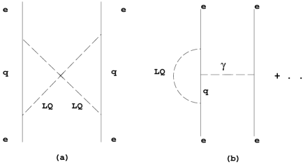
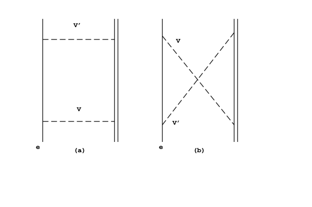
FIG. 1.: Leptoquark (LQ) one-loop contributions to PV Möller scattering.

FIG. 2.: Two vector boson exchange dispersion corrections. Here $V$ and $V^{\prime}$ denote $\gamma$, $Z^{0}$, or $W^{\pm}$. Double vertical line denotes hadronic target.

- [1] See, for example, D. Schaile, “-pole Experiments”, in Precision Tests of the Standard Electroweak Model, P. Langacker, Ed., World Scientific, Singapore, 1995, p. 545.
- [2] J.L. Rosner, Comments in Nucl. Part. Phys. 22 (1998) 205
- [3] See, e.g., A. Deandrea, [hep-ph/9705435]; V. Barger, et al., [hep-ph/9710353].
- [4] A.E. Nelson, Phys. Rev. Lett. 78 (1997) 4159.
- [5] C.S. Wood et al., Science 275 (1997) 1759.
- [6] D. Chauvat, et al., Eur. Phys. J. D1 (1998) 169.
- [7] E.N. Fortson, Phys. Rev. Lett. 70 (1993) 2383.
- [8] D. Budker, “Parity Nonconservation in Atoms”, to appear in proceedings of WEIN-98, C. Hoffman and D. Herzceg, Eds., World Scientific, Singapore, 1998.
- [9] D. DeMille, Phys. Rev. Lett. 74 (1995) 4165.
- [10] C.Y. Prescott et al., Phys. Lett. B77 (1978) 347; Phys. Lett. B84 (1979) 524.
- [11] W. Heil et al., Nucl. Phys. B327 (1989) 1.
- [12] P.A. Souder et al., Phys. Rev. Lett. 65 (1990) 694.
- [13] MIT-Bates experiment 89-06 (1989), R.D. McKeown and D.H. Beck spokespersons; MIT-Bates experiment 94-11 (1994), M. Pitt and E.J. Beise, spokespersons; Jefferson Lab experiment E-91-017 (1991), D.H. Beck, spokesperson; Jefferson Lab experiment E-91-004 (1991), E.J. Beise, spokesperson; Jefferson Lab experiment E-91-010 (1991), M. Finn and P.A. Souder, spokespersons; Mainz experiment A4/1-93 (1993), D. von Harrach, spokesperson
- [14] B. Mueller et al., SAMPLE Collaboration, Phys. Rev. Lett. 78 (1997) 3824
- [15] K.A. Aniol et al., HAPPEX Collaboration, [nucl-ex/9810012]
- [16] Proceedings of the 1997 summer Jefferson Laboratory-Institute for Nuclear Theory workshop “Future Directions in Parity-Violation”, R. Carlini and M.J. Ramsey-Musolf, Eds. (unpublished).
- [17] SLAC Proposal E158 (1997), K. Kumar, spokesperson.
- [18] P.A. Souder, private communication.
- [19] M.E. Peskin and T. Takeuchi, Phys. Rev. Lett. 65 (1990) 964.
- [20] W.J. Marciano and J.L. Rosner, Phys. Rev. Lett. 65 (1990) 2963.
- [21] M.J. Musolf et al., Phys. Rep. 239 (1994) 1.
- [22] G. Feinberg, Phys. Rev. D12 (1975) 3575.
- [23] J.D. Walecka, Nucl. Phys. A285 (1977) 349.
- [24] N. Mukhopadhyay et al., Nucl. Phys. A633 (1998) 481.
- [25] E.N. Fortson, Y. Pang, L. Wilets, Phys. Rev. Lett. 65 (1990) 2857.
- [26] S.J. Pollock, E.N. Fortson, L. Wilets, Phys. Rev. C46 (1992) 2587.
- [27] B.Q. Chen and P. Vogel, Phys. Rev. C48 (1993) 1392.
- [28] P. Vogel, “Atomic Parity Non-conservation and Nuclear Structure” in Nuclear Shapes and Nuclear Structure, M. Vergnes, D. Goute, P.H. Heenen, and J. Sauvage, Eds., Edition Frontieres, 1994, Gif-sur-Yvette.
- [29] M.J. Musolf and B.R. Holstein, Phys. Lett. B242 (1990) 461.
- [30] SLAC Proposal E149 (1992) P. Bosted, spokesperson.
- [31] SLAC Proposal E149 (1993) P. Bosted, spokesperson.
- [32] B.P. Masterson and C.E. Wieman, “Atomic Parity Nonconservation Experiments”, in Precision Tests of the Standard Electroweak Model, P. Langacker, Ed., World Scientific, Singapore, 1995, p. 545.
- [33] Particle Data Group, Review of Particle Properties, Z. Phys. C3 (1998) 1.
- [34] A. Czarnecki and W.J. Marciano, Phys. Rev. D53 (1996) 1066.
- [35] M.J. Musolf and T.W Donnelly, Nucl. Phys. A546 (1992) 509; A550 (1992) 564 (E).
- [36] T. Rizzo, “Searches for New Gauge Bosons at Future Colliders”, in Proceedings of the 1996 DPF/DPB Summer Study on New Directions for High Energy Physics-Snowmass 96, Sowmass, CO, 1996 [hep-ph/9609248].
- [37] T. Rizzo, “Searches for Scalar and Vector Leptoquarks at Future Colliders”, in Proceedings of the 1996 DPF/DPB Summer Study on New Directions for High Energy Physics-Snowmass 96, Sowmass, CO, 1996 [hep-ph/9609267].
- [38] E.N. Fortson in Ref. [16].
- [39] D. London and J.L. Rosner, Phys. Rev. D34 (1986) 1530.
- [40] P. Langacker, M. Luo, and A.K. Mann, Rev. Mod. Phys. 64 (1992) 87.
- [41] P. Langacker, “Tests of the Standard Model and Searches for New Physics”, in Precision Tests of the Standard Electroweak Model, P. Langacker, Ed., World Scientific, Signapore, 1995, p.883.
- [42] R.N. Mohapatra, Unification and Supersymmetry, Springer-Verlag, New York, 1992.
- [43] F. Abe et al., CDF Collaboration, Phys. Rev. Lett. 79 (1997) 2192.
- [44] C. Adloff et al., H1 Collaboration, Z. Phys. C74 (1997) 191.
- [45] J. Breitweg et al., ZEUS Collaboration, Z. Phys. C74 (1997) 207.
- [46] J.L. Hewett and T.G. Rizzo, Phys. Rev. D56 (1997) 5709.
- [47] See, for example, G. Altarelli [hep-ph/9708437]; K.S. Babu, C. Kolda, J. March-Russell, Phys. Lett. B402 (1997) 367; ibid B408 (1997) 261; J. Blumlein, Z. Phys. C74 (1997) 605 and references therein.
- [48] J. Hobbs, (D0 Collaboration), talk presented at 32nd Rencontres de Moriond: Electroweak Interactions and Unified Theories, Le Arces, France, March 1997; F. Abe et al., (CDF Collaboration), Fermilab Report FNAL-PUB-96-450-E.
- [49] See, e.g., J. Hewett [hep-ph/9310361]; G. Altarelli, Ref. [47] below.
- [50] B. Abbott, et al., (D0 Collaboration), Phys. Rev. Lett. 80 (1998) 2051.
- [51] J.L. Hewett and T.G. Rizzo, Phys. Rev. D58 (1998) 055005.
- [52] V. Barger, G.F. Guidice, T. Han, Phys. Rev. D40 (1989) 2987.
- [53] T. Kon and T. Kobayashi [hep-ph/9704221].
- [54] D. Choudhury and S. Raychaudhuri [hep-ph/9702392].
- [55] M. Hirsch, H.V. Klapdor-Kleingrothaus, and S.G. Kovalenko, Phys. Rev. D53 (1996) 1329.
- [56] I.S. Towner and J.C. Hardy, “Currents and their Couplings in the Weak Sector of the Standard Model”, in Symmetries and Fundamental Interactions in Nuclei, W.C. Haxton and E.M. Henley, Eds., World Scientific, Singapore, 1995, p. 183.
- [57] E. Hagberg et al., in Non-Nucleonic Degrees of Freedom Detected in the Nucleus, T. Minamisono et al., Eds., World Scientific, 1996, Singapore.
- [58] B.K. Fujikawa et al., [nucl-ex/9806001].
- [59] F. Abe et al., CDF Collaboration, Phys. Rev. Lett. 79 (1997) 2198.
- [60] See, for example, E. Eichten, K.D. Lane, and M.E. Peskin, Phys. Rev. Lett. 50 (1983) 811; A.E. Nelson, Phys. Rev. Lett. 78 (1997) 4159 and references therein. Vector Leptoquarks Study on New [hep-ph/9609267].
- [61] K. Ackerstaff et al., OPAL Collaboration, Phys. Lett. B391 (1997) 221.
- [62] A. Bodek for the CDF Collaboration, “Limits on Quark-Lepton Compositeness and Studies on W Asymmetry at the Tevatron Collider”, talk presented at 28th International Conference on High-energy Physics (ICHEP 96), Warsaw, Poland, July 1996. Published in ICHEP 96:1438-1441.
- [63] W. Buchmüller and D. Wyler, [hep-ph/9704317]
- [64] V.A. Dzuba, V.V. Flambaum, and O.P. Sushkov, Phys. Lett. A141 (1989) 147.
- [65] S.A. Blundell, J. Sapirstein, W.R. Johnson, Phys. Rev. D45 (1992) 1602.
- [66] T.W. Donnelly, J. Duback, I. Sick, Nucl. Phys. A503 (1989) 589.
- [67] C.J. Horowitz, Phys. Rev. C57 (1998) 3430.
- [68] R. Carlini and P. Souder, private communication.
- [69] Jefferson Lab experiment E-91-010 (1991), M. Finn and P.A. Souder, spokespersons.
- [70] Mainz experiment A4/1-93 (1993), D. von Harrach, spokesperson.
- [71] M.J. Musolf and T.W. Donnelly, Z. Phys. C57 (1993) 559.
- [72] W.J. Maricano and A. Sirlin, Phys. Rev. D27 (1983) 552; D29 (1984) 75.