Abstract

We make a global vacuum neutrino oscillation analysis of solar neutrino data, including the seasonal and energy dependence of the recent Super–Kamiokande 708-day results. The best fit parameters for $\nu_{e}$ oscillations to an active neutrino are $\delta m^{2}=4.42\times 10^{-10}$ eV², $\sin^{2}2\theta=0.93$. The allowed mixing angle region is consistent with bi–maximal mixing of three neutrinos. Oscillations to a sterile neutrino are disfavored. Allowing an enhanced $hep$ neutrino flux does not significantly alter the oscillation parameters.

1 Introduction

For quite some time, measurements of solar neutrinos [1, 2] have indicated a suppression compared to the expectations of the standard solar model (SSM) [3]. This suppression may be explained by assuming that $\nu_{e}$ from the Sun undergo vacuum oscillations as they travel to the Earth [4, 5]. Recent data from the Super–Kamiokande (SuperK) experiment [6] also exhibit a seasonal variation above that expected from the $1/(\rm distance)^{2}$ dependence of the neutrino flux, which if verified would be a clear signal of vacuum oscillations[7, 8, 9].

In this Letter we determine the best fit vacuum oscillation parameters to the combined solar neutrino data, including the 708–day SuperK observations. For oscillations to an active neutrino there are subtle changes in the allowed regions compared to fits with earlier SuperK data [9, 10]. Oscillations to a sterile neutrino are disfavored. We examine the possibility that the solar $hep$ neutrino flux is enhanced compared to the SSM, and find that the best fits are only marginally changed. We also find a solution with very low $\delta m^{2}\simeq 6\times 10^{-12}$ eV² for oscillations to a sterile neutrino or with an $hep$ enhancement.

2 Fitting procedure

The fitting procedure is described in detail in Ref. [9]. The solar data used in the current fit are the ³⁷Cl (1 data point) and ⁷¹Ga (2 data points) capture rates [1], the latest SuperK electron recoil energy spectrum with $E_{e}$ in the range 5.5 to 20 MeV [6] (18 data points), and the latest seasonal variation data from SuperK for $E_{e}$ in the range 11.5 to 20 MeV [6] (8 data points). For $\nu_{e}$ oscillations to an active neutrino ($\nu_{\mu}$ or $\nu_{\tau}$) we take into account the neutral current interactions in the SuperK experiment. We fold the SuperK electron energy resolution [2] in the oscillation predictions for the $E_{e}$ distribution. For all rates that are annual averages we integrate over the variation in the Earth-Sun distance. We do not include the SuperK day/night ratio, since it is unity for vacuum oscillations.

To allow for uncertainty in the SSM prediction of the ⁸B neutrino flux, we include as a free parameter $\beta$, the ⁸B neutrino flux normalization relative to SSM prediction. In our fits with non–standard $hep$ neutrinos we also include an arbitrary $hep$ normalization constant, $\gamma$. For the SSM predictions we adopt the results of Ref. [3].

3 Solutions with oscillations to an active neutrino

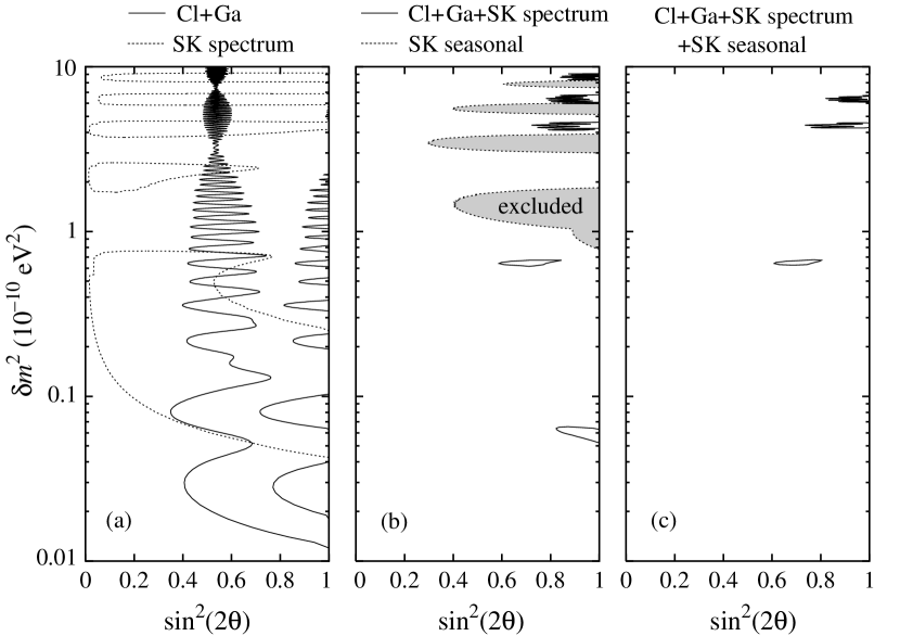
Figure 1: Regions in $\sin^{2}2\theta$–$\delta m^{2}$ parameter space (a) allowed at 95% C.L. by the ³⁷Cl and ⁷¹Ga capture rates (solid curve) and the Super–Kamiokande $E_{e}$ spectrum (dotted), (b) allowed at 95% C.L. by the combined ³⁷Cl and ⁷¹Ga capture rates and Super–Kamiokande $E_{e}$ spectrum (solid) and excluded at 68% C.L. by the Super–Kamiokande seasonal data (shaded), and (c) allowed at 95% C.L. by all the data.

Figure 1a shows the 95% C.L. allowed regions for the combined radiochemical (³⁷Cl and ⁷¹Ga) capture rates and the SuperK electron recoil spectrum, including its normalization. For the 95% C.L. region in a three–parameter fit ($\delta m^{2},\sin^{2}2\theta,\beta$) we include all solutions with $\chi^{2}<\chi^{2}_{min}+8$. On the boundary curves of the fit to the radiochemical data, the faster oscillations are due to the lower energy neutrinos (mainly $pp$ and ⁷Be), and the slower oscillations are due to the ⁸B neutrinos. The five regions allowed by the SuperK spectrum data correspond roughly to having a mean Earth–Sun distance equal to (in increasing order of $\delta m^{2}$) ${1\over 2}$, ${3\over 2}$, ${5\over 2}$, ${7\over 2}$, or ${9\over 2}$ oscillation wavelengths for a typical ⁸B neutrino energy. Following the notation of Ref. [9], we label these regions A, B, C, D, and E, in order of ascending $\delta m^{2}$.

In Figure 1b we show the allowed regions for the combined radiochemical and SuperK spectrum data (the solid curve). Also shown in Fig. 1b is the region excluded by the seasonal SuperK data at 68% C.L. (we show the 68% C.L. region since almost none of the parameter space is excluded by the seasonal variation at 95% C.L.).

Finally, in Fig. 1c we show the 95% C.L. allowed regions obtained with all of the data (radiochemical, SuperK spectrum, and SuperK seasonal). Only regions A, C, and D are allowed at 95% C.L. by the combined data set. The best fits in each of the subregions are shown in Table 1. Region B, which was allowed in previous fits [9, 10], is now excluded. The overall best fit parameters are in region C

$$\delta m^{2}=4.42\times 10^{-10}{\rm~{}eV}^{2}\,,\qquad\sin^{2}2\theta=0.93\,,\qquad\beta=0.78\,,$$ (1)

with $\chi^{2}/DOF=33.8/26$, which corresponds to a goodness–of–fit of 14% (the goodness–of–fit is the probability that a random repeat of the given experiment would observe a greater $\chi^{2}$, assuming the model is correct). The next best fit is in region $D$ with

$$\delta m^{2}=6.44\times 10^{-10}{\rm~{}eV}^{2}\,,\qquad\sin^{2}2\theta=1.00\,,\qquad\beta=0.80\,,$$ (2)

with $\chi^{2}/DOF=36.7/26$, which corresponds to a goodness–of–fit of 8%. Finally, region A is also allowed, with best fit

$$\delta m^{2}=6.5\times 10^{-11}{\rm~{}eV}^{2}\,,\qquad\sin^{2}2\theta=0.70\,,\qquad\beta=0.94\,,$$ (3)

with $\chi^{2}/DOF=38.4/26$, which corresponds to a goodness–of–fit of 6%. Regions C and D are consistent with bi–maximal[11] or nearly bi–maximal[12] three–neutrino mixing models that can describe both solar and atmospheric neutrino data. Regions B and E are excluded at 95% C.L.

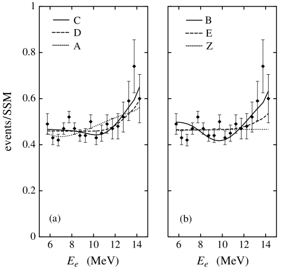
Figure 2: Ratio of predicted $E_{e}$ spectrum in Super–Kamiokande to the SSM for (a) models favored by a global fit, C (solid curve), D (dashed), and A (dotted), and (b) models disfavored by a global fit, B (solid), E (dashed) and Z (dotted).

We see from Table 1 that generally the higher $\delta m^{2}$ solutions fit the $E_{e}$ spectrum better. This is evident in Fig. 2, which shows the $E_{e}$ spectrum predictions for the solutions in Table 1, and the latest SuperK data [6]. The higher $\delta m^{2}$ solutions do worse for the radiochemical experiments, primarily because the seasonal variation in the oscillation argument is larger in these cases for the ⁷Be neutrinos, causing more smearing of the oscillation probability. The annual–averaged suppression of ⁷Be neutrinos is about 93% for solution A, 66% for solutions B and C, and 57% for solutions D and E. The best fit in each region generally lies near a local minimum for the ⁷Be neutrino contribution, as might be expected from model independent analyses without oscillations that indicate suppression of ⁷Be contributions [13].

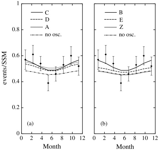
Figure 3: Ratio of predicted rate to SSM prediction versus time of year in Super–Kamiokande for (a) models favored by a global fit, C (solid curve), D (dashed), and A (dotted), and (b) models disfavored a by global fit, B (solid), E(dashed), and Z (dashed). Results for no oscillations with ⁸B normalization of 0.47 are shown by the dash-dotted curves.

Results for the seasonal variation of the solutions in Table 1 are shown in Fig. 3, along with the latest SuperK data [6]. Also shown is the best fit for no oscillations with arbitrary ⁸B neutrino normalization; the latter has a small seasonal dependence due to the variation of the Earth-Sun distance. Current seasonal data do not provide a strong constraint, but clearly solutions A, C, and D fit the data better than the no–oscillation curve.

Also included in Table 1 is a solution with very low $\delta m^{2}$, which we call solution Z, that was pointed out in Ref. [14]. It is excluded at 95% C.L., but marginally allowed at 99% C.L. (as is solution B). It corresponds roughly to a mean Earth–Sun distance equal to ${1\over 2}$ of the oscillation wavelength (maximal supression) for ⁷Be neutrinos. Although it does very well in suppressing the ⁷Be neutrinos (by about 94% after accounting for seasonal averaging), it does not show a significant seasonal effect beyond that provided by the variation of the Earth-Sun distance (see Fig. 3b).

4 Solutions with oscillations to a sterile neutrino

A similar analysis may be made with solar $\nu_{e}$ oscillating into a sterile neutrino species. Since the sterile neutrino does not interact in any of the detectors, it is harder to reconcile the differing rates of the ³⁷Cl and SuperK experiments [7]. The best fit parameters in each of the regions are shown in Table 2. For sterile neutrinos the overall best fit parameter is again in region C with $\chi^{2}/DOF=42.4/26$, which is excluded at 97.7% C.L. Therefore oscillations to sterile neutrinos are highly disfavored. Interestingly, the fit for solution Z is comparable to the other best–fit solutions in the sterile case because its strong suppression of ⁷Be neutrinos helps account for the difference between the ³⁷Cl and SuperK rates (note the $\chi^{2}$ values for the ³⁷Cl data in Table 2).

5 Solutions with non-standard contributions from $hep$ neutrinos

Recently it has been speculated that the rise in the SuperK $E_{e}$ spectrum at higher energies could be due to a larger than expected $hep$ neutrino flux contribution [15, 16]. While the maximum energy of the ⁸B neutrinos is about 15 MeV, the $hep$ neutrinos have maximum energy of 18.8 MeV. In the SSM the total flux of ⁸B neutrinos is about 2000 times that of the $hep$ neutrinos [3], and the $hep$ contribution to the SuperK experiment is negligible. However, there is a large uncertainty in the low energy cross section for the reaction ${}^{3}He+p\rightarrow^{4}He+e^{+}+\nu_{e}$ in which the $hep$ neutrinos are produced, and an $hep$ flux much larger than the SSM value may not be unreasonable [15, 16]. A large enhancement of the $hep$ contribution could in principle account for the rise in the $E_{e}$ spectrum at higher energies seen by SuperK. The $hep$ flux normalization $\gamma$ can be determined once there are sufficient events in the region $E_{e}>15$ MeV. SuperK measurements of the $E_{e}$ spectrum in the range 17–25 MeV already place the upper limit $\gamma<8$ at 90% C.L. [6], assuming no oscillations.

It should first be noted that although an enhanced $hep$ contribution without neutrino oscillations can provide a good fit to the SuperK data for $5.5<E_{e}<14$ MeV, it cannot also account for the ³⁷Cl and ⁷¹Ga rates even with arbitrary ⁸B, $hep$, and ⁷Be neutrino flux normalizations. The overall best fit in this case occurs with no ⁷Be contribution, and has $\chi^{2}/DOF=53.7/26$, which is excluded at 99.9% C.L. The contributions of the $pp$ neutrinos, plus the reduced amount of ⁸B neutrinos needed to explain SuperK, give a rate for the radiochemical experiments that is too high, even when the ⁷Be contribution is ignored.

One can also ask what happens if an enhanced $hep$ contribution is combined with neutrino oscillations [16], although the motivation for enhancing the $hep$ neutrino flux is not strong here since vacuum oscillations already can explain the rise in the SuperK $E_{e}$ spectrum. Table 3 shows the best fits in each region when an arbitrary $\gamma$ is allowed. The overall best fit parameters in this case are again in region C with $\chi^{2}/DOF=32.8/25$, which corresponds to a goodness–of–fit of 14%. The fits for most of the regions are not significantly improved from the standard $hep$ flux case, and the fitted oscillation parameters are little changed. The only exceptions are solutions E and Z, which originally could not explain the SuperK spectrum as well, but with the addition of extra $hep$ neutrinos can now also provide a reasonable fit to all of the data. Regions A, C, D, E, and Z are all allowed at 95% C.L. when an $hep$ enhancement is included. However, the preferred values of $\gamma$ exceed the current bound from SuperK, so that the role of an $hep$ flux enhancement appears to be minimal.

6 Summary and discussion

The latest SuperK solar neutrino data suggest there is a seasonal variation in the solar neutrino flux. The hypothesis that solar $\nu_{e}$ undergo vacuum oscillations to an active neutrino species provides a consistent explanation of all the solar data, with a best fit given by oscillation parameters $\delta m^{2}=4.42\times 10^{-10}$ eV² and $\sin^{2}2\theta=0.93$. Oscillations to sterile neutrinos are ruled out at 97.7% C.L., and fits with an enhanced $hep$ neutrino flux do not significantly alter the fit results.

The existence of vacuum neutrino oscillations can be confirmed with more data from SuperK on the seasonal variation of the ⁸B neutrino flux. The spectrum and seasonal variations of ⁸B neutrinos can also be measured in the Sudbury Neutrino Observatory (SNO) [17] and ICARUS [18] experiments. The line spectrum of the ⁷Be neutrinos gives larger seasonal variations than ⁸B [7, 8] and these may be observable with increased statistics in ⁷¹Ga experiments, or in the BOREXINO experiment[19], for which ⁷Be neutrinos provide the dominant signal. Accurate measurements of the seasonal variation in these experiments should be able to distinguish between the different vacuum oscillation scenarios [9], providing a unique solution to the solar neutrino problem.

Table 1: Best fit parameters and $\chi^{2}$ for various vacuum oscillation solutions with $\nu_{e}$ oscillations to an active neutrino.

	Parameters					$\chi^{2}$		$\chi^{2}$
Solution	$\delta m^{2}$	$\sin^{2}2\theta$	$\beta$	37Cl	71Ga	spectrum	seasonal	total
	($10^{-10}$ eV2)
A	0.65	0.70	0.95	4.7	1.2	25.8	6.7	38.4
B	2.49	0.80	0.79	8.9	1.1	30.4	5.4	45.8
C	4.42	0.93	0.78	6.7	4.4	17.4	5.3	33.8
D	6.44	1.00	0.80	7.5	5.2	17.6	6.4	36.7
E	8.61	1.00	0.81	7.7	5.3	20.4	8.7	42.1
Z	0.06	1.00	0.47	5.0	2.5	24.8	13.3	45.6

Table 2: Best fit parameters and $\chi^{2}$ for various vacuum oscillation solutions with $\nu_{e}$ oscillations to a sterile neutrino.

	Parameters					$\chi^{2}$		$\chi^{2}$
Solution	$\delta m^{2}$	$\sin^{2}2\theta$	$\beta$	37Cl	71Ga	spectrum	seasonal	total
	($10^{-10}$ eV2)
A	0.64	0.62	0.96	18.9	1.4	29.3	6.7	56.3
B	2.49	0.73	0.82	21.2	1.4	33.1	5.3	61.0
C	4.42	0.89	0.84	15.8	2.7	18.5	5.4	42.4
D	6.42	0.97	0.88	15.3	5.2	17.3	5.9	43.7
E	8.62	1.00	0.91	15.7	5.5	19.2	8.1	48.5
Z	0.06	1.00	0.48	6.2	2.4	25.5	11.5	45.6

Table 3: Best fit parameters and $\chi^{2}$ for various vacuum oscillation solutions with $\nu_{e}$ oscillations to an active neutrino and a non–standard $hep$ contribution $\gamma$ times the SSM prediction.

	Parameters						$\chi^{2}$		$\chi^{2}$
Solution	$\delta m^{2}$	$\sin^{2}2\theta$	$\beta$	$\gamma$	37Cl	71Ga	spectrum	seasonal	total
	($10^{-10}$ eV2)
A	0.65	0.70	0.94	7	4.4	1.3	26.0	6.7	38.3
B	2.50	0.76	0.74	38	8.5	1.1	27.9	5.8	43.2
C	4.42	0.90	0.74	35	6.2	3.4	17.6	5.6	32.8
D	6.44	0.98	0.76	50	6.2	4.5	17.4	7.1	33.2
E	8.61	0.97	0.75	66	5.9	4.3	18.4	10.3	38.9
Z	0.06	0.98	0.44	52	2.7	2.2	19.3	14.9	39.1

References

- [1] B.T. Cleveland et al., Nucl. Phys. B (Proc. Suppl.) 38, 47 (1995); GALLEX collaboration, W. Hampel et al., Phys. Lett. B388, 384 (1996); SAGE collaboration, J.N. Abdurashitov et al., Phys. Rev. Lett. 77, 4708 (1996).
- [2] Kamiokande collaboration, Y. Fukuda et al., Phys. Rev. Lett, 77, 1683 (1996); Super–Kamiokande collaboration, Y. Suzuki, talk at Neutrino–98, Takayama, Japan, June 1998.
- [3] See, e.g., J.N. Bahcall, S. Basu, and M.H. Pinsonneault, Phys. Lett. B 433, 1 (1998), and references therein.
- [4] V. Barger, R.J.N. Phillips, and K. Whisnant, Phys. Rev. D 24, 538 (1981).
- [5] S.L. Glashow and L.M. Krauss, Phys. Lett. B190, 199 (1987).
- [6] M.B. Smy, talk at DPF-99, Los Angeles, California, January 1999; G. Sullivan, talk at Aspen Winter Conference, January, 1999.
- [7] V. Barger, R.J.N. Phillips, and K. Whisnant, Phys. Rev. Lett. 65, 3084 (1990); ibid. 69, 3135 (1992); P.I. Krastev and S.T. Petcov, Phys. Lett. B 285, 85 (1992); Nucl. Phys. B449, 605 (1995);
- [8] S. Pakvasa and J. Pantaleone, Phys. Rev. Lett. 65, 2479 (1990); A. Acker, S. Pakvasa, and J. Pantaleone, Phys. Rev. D 43, 1754 (1991); S.P. Mikheyev and A.Yu. Smirnov, Phys. Lett. B429, 343 (1998); B. Faid, G.L. Fogli, E. Lisi, and D. Montanino, Astropart. Phys. 10, 93 (1999); S.L. Glashow, P.J. Kernan, and L.M. Krauss, Phys. Lett. B445, 412 (1999); J.M. Gelb and S.P. Rosen, hep-ph/9809508; V. Berezinsky, G. Fiorentini, and M. Lissia, hep-ph/9811352;
- [9] V. Barger and K. Whisnant, hep/ph-9812273, to appear in Phys. Rev. D.
- [10] J.N. Bahcall, P.I. Krastev, and A.Yu. Smirnov, Phys. Rev. D 58, 096016 (1998).
- [11] V. Barger, S. Pakvasa, T.J. Weiler, and K. Whisnant, Phys. Lett. B 437, 107 (1998); A.J. Baltz, A. Goldhaber, and M. Goldhaber, Phys. Rev. Lett. 81, 5730 (1998); M. Jezabek and Y. Sumino, Phys. Lett. B 440, 327 (1998); Y. Nomura and T. Yanagida, Phys. Rev. D 59, 017303 (1999); G. Altarelli and F. Feruglio, Phys. Lett. B439, 112 (1998); JHEP 11, 021 (1998); H. Georgi and S. Glashow, hep-ph/9808293; S. Davidson and S.F. King, Phys. Lett. B 445, 191 (1998); R.N. Mohapatra and S. Nussinov, Phys. Lett. B441, 299 (1998); hep-ph/9809415; S.K. Kang and C.S. Kim, hep-ph/9811379; C. Jarlskog, M. Matsuda, S. Skadhauge, and M. Tanimoto, hep-ph/9812282; E. Ma, hep-ph/9812344.
- [12] H. Fritzsch and Z. Xing, Phys. Lett. B372, 265 (1996); 440, 313 (1998); E. Torrente-Lujan, Phys. Lett. B389, 557 (1996); M. Fukugita, M. Tanimoto, and T. Yanagida, Phys. Rev. D57, 4429 (1998); M. Tanimoto, Phys. Rev. D 59, 017304 (1999).
- [13] J.N. Bahcall and H. Bethe, Phys. Rev. 47, 1298 (1993); P. Rosen and W. Kwong, Phys. Rev. Lett. 73, 369 (1994); J.N. Bahcall, Phys. Lett. B 338, 276(1994); S. Parke, Phys. Rev. Lett. 74, 839 (1995); N. Hata and P. Langacker, Phys. Rev. D 52, 420 (1995); H. Minakata and H. Nunokawa, hep-ph/9902460.
- [14] P.I. Krastev and S.T. Petcov, Phys. Rev. D 53, 1665 (1996).
- [15] R. Escribano, J.M. Frere, A. Gevaert, and D. Monderen, Phys. Lett. B 444, 397 (1998).
- [16] J.N. Bahcall and P.I. Krastev, Phys. Lett. B 436, 243 (1998).
- [17] A. McDonald, Solar Neutrino Observatory (SNO) collaboration, talk at Neutrino–98, Takayama, Japan, June 1998.
- [18] ICARUS collaboration, F. Arneodo et al., Nucl. Phys. Proc. Suppl. 70, 453 (1999).
- [19] L. Oberauer, BOREXINO Collaboration, talk at Neutrino–98, Takayama, Japan, June 1998.