CERN-TH/99-57

DTP/99/26

hep-ph/9903260

March 1999

Top quark production near threshold
and the top quark mass
M. Beneke Theory Division, CERN, CH-1211 Geneva 23, Switzerland
A. Signer Department of Physics, University of Durham,
Durham DH1 3LE, England
V.A. Smirnov Nuclear Physics Institute, Moscow State University,
119889 Moscow, Russia

We consider top-anti-top production near threshold in $e^{+}e^{-}$ collisions, resumming Coulomb-enhanced corrections at next-to-next-to-leading order (NNLO). We also sum potentially large logarithms of the small top quark velocity at the next-to-leading logarithmic level using the renormalization group. The NNLO correction to the cross section is large, and it leads to a significant modification of the peak position and normalization. We demonstrate that an accurate top quark mass determination is feasible if one abandons the conventional pole mass scheme and if one uses a subtracted potential and the corresponding mass definition. Significant uncertainties in the normalization of the $t\bar{t}$ cross section, however, remain.

1. Introduction. The top quark mass is now known to be around $175\,$GeV with an accuracy of $5\,$GeV from the direct measurement at the Fermilab Tevatron Collider [1]. Accurate mass determinations (with errors below 1-2 GeV) are difficult at hadron colliders. Despite the fact that orders of magnitudes more top quarks will be produced at the CERN Large Hadron Collider, a precision measurement is reserved for a future lepton collider. In this case the method of choice relies on scanning the top quark pair production threshold. From an experimental point of view, an error in the $100\,$MeV range is conceivable [2]; the limiting factor is the accuracy to which the cross section can be predicted theoretically as a function of the top quark mass.

The literature on top quark physics near threshold in $e^{+}e^{-}$ collisions is substantial [3, 4]. Perturbative calculations in the threshold region require that either the toponium Rydberg energy scale $m_{t}\alpha_{s}^{2}\gg\Lambda_{\rm QCD}$ or that the top quark decay width $\Gamma_{t}\gg\Lambda_{\rm QCD}$. Both conditions are satisfied and since $\Gamma_{t}\sim m_{t}\alpha_{s}^{2}\sim 1.5\,$GeV, narrow toponium resonances do not exist [5]. In the kinematic region of interest, the top quarks are slow, with typical velocities $v\sim 1/10$. As a consequence methods familiar from non-relativistic bound state calculations in QED can be used to compute the $t\bar{t}$ cross section. In particular, the dominant interaction between the $t$ and $\bar{t}$ can be described by the colour-singlet Coulomb potential, which has to be treated non-perturbatively [3]. Corrections are computed in the background of this strong Coulomb interaction.

Recently, the 2-loop QCD correction to the Coulomb potential [6] (correcting an earlier result [7]) and the 2-loop relativistic correction to the $t\bar{t}$ vector coupling to the initial virtual photon or $Z$ boson [8, 9] have been computed. With these two inputs at hand, we can compute the next-to-next-to-leading order (NNLO) QCD correction to the top quark pair production cross section. (The precise meaning of ‘NNLO’ in the present context is given below.) In the following, we first compute the NNLO QCD correction in the conventional pole mass scheme, i.e. the threshold cross section is expressed in terms of the top quark pole mass. Comparable calculations, with some technical and implementational differences, have already been completed by several groups [10, 11, 12]. We find that the NNLO correction is substantial and leads to an uncomfortably large shift in the top quark mass, raising questions as to the stability of the theoretical prediction. In [13], one of us suggested that such shifts could occur as a consequence of on-shell mass renormalization, which is particularly (and in the case at hand, artificially) sensitive to non-perturbative, long-distance effects. This sensitivity to non-perturbative effects can be removed by using a different mass renormalization scheme (called the potential subtraction (PS) scheme in [13]) with the additional benefit that the new mass definition can also be related more reliably to short-distance masses (such as the $\overline{\rm MS}$ mass), which are ultimately of more interest for high-energy processes and Yukawa coupling unification relations (should they exist).

The main result of this letter is to demonstrate that this procedure works. We show that the mass shifts become small in the PS scheme, and that the PS mass can also be accurately related to the $\overline{\rm MS}$ mass. However, the normalization uncertainty of the cross section remains large, and is larger than could have been anticipated from the earlier next-to-leading order (NLO) calculations. The second improvement which we suggest in this letter is to use renormalization group equations to sum large logarithms, $\ln v$ and $\ln v^{2}$ to all orders in perturbation theory. The consideration of logarithms is important to identify correctly the scales of the various subprocesses, but not restricted to the scale of the QCD coupling only. In the present work, we complete this program (almost trivially) to the next-to-leading logarithmic (NLL) order. The step to NNLL is substantially more complicated and we will discuss it, together with the details of the present calculation, in a future publication [14].

Before proceeding, let us emphasize that ‘NLO’, ‘NNLO’ etc. do not refer to a conventional loop expansion in $\alpha_{s}$, because the Coulomb interaction cannot be treated perturbatively in the threshold region. To be precise, a LO, NLO, … approximation to the normalized cross section takes into account all terms of order

$$R\equiv\sigma_{t\bar{t}}/\sigma_{\mu^{+}\mu^{-}}=v\,\sum_{k}\left(\frac{\alpha_{s}}{v}\right)^{k}\cdot\left\{1\,\mbox{(LO)};\,\alpha_{s},v\,\mbox{(NLO)};\,\alpha_{s}^{2},\alpha_{s}v,v^{2}\,\mbox{(NNLO)};\,\ldots\right\},$$ (1)

where logarithms of $v$ are suppressed. The renormalization group improved treatment extends this to the summation of logarithms such that a LL, NLL, … approximation accounts for all terms of order

$$R=v\,\sum_{k}\left(\frac{\alpha_{s}}{v}\right)^{k}\sum_{l}\left(\alpha_{s}\ln v\right)^{l}\cdot\left\{1\,\mbox{(LL)};\,\alpha_{s},v\,\mbox{(NLL)};\,\alpha_{s}^{2},\alpha_{s}v,v^{2}\,\mbox{(NNLL)};\,\ldots\right\}.$$ (2)

The result discussed here is complete at ‘NNLO’ and ‘NLL’. Furthermore, near the would-be toponium poles another resummation is necessary, which we discuss below.

We also emphasize that the NNLO QCD correction is defined as above in the limit $\Gamma_{t}\ll m_{t}\alpha_{s}^{2}$. When $\Gamma_{t}\sim m_{t}\alpha_{s}^{2}$, as we expect, further corrections arise from so-called non-factorizable contributions [15], which have not been calculated so far with the Coulomb interaction treated non-perturbatively. Electroweak corrections also enter and the entire concept of a $t\bar{t}$ cross section has to be revised, since single resonant contributions are expected to contribute at NNLO (in the above power counting scheme with $\Gamma_{t}\sim m_{t}\alpha_{s}^{2}$) to the $WWb\bar{b}$ final state. These are interesting issues to be studied, but we expect them to bear little on the issue of an accurate top mass determination which we address in this letter. Hence, we will keep the top quark width only in the form of an imaginary mass term $i\Gamma_{t}\psi^{\dagger}\psi$ for the non-relativistic top quarks; this amounts to evaluating the $t\bar{t}$ Green function at energy $E+i\Gamma_{t}$ as familiar from LO and NLO calculations [3, 4]. As a final (trivial) simplification, we restrict our attention to $t\bar{t}$ pairs produced through the vector coupling to a virtual photon. The vector coupling to a $Z$ boson can be accommodated by a trivial replacement of the electric charge. The axial vector coupling is suppressed by a factor of $v^{2}$ near threshold; no QCD corrections to it are needed at NNLO.

2. Derivation of the cross section. With the treatment of the top quark width as specified above, and neglecting the axial-vector coupling, the $t\bar{t}$ production cross section is obtained from the correlation function

$$\Pi_{\mu\nu}(q^{2})=(q_{\mu}q_{\nu}-q^{2}g_{\mu\nu})\,\Pi(q^{2})=i\int d^{4}x\,e^{iq\cdot x}\,\langle 0|T(j_{\mu}(x)j_{\nu}(0))|0\rangle,$$ (3)

where $j^{\mu}(x)=[\bar{t}\gamma^{\mu}t](x)$ is the top quark vector current and $s=q^{2}$ the centre-of-mass energy squared. Defining the usual $R$-ratio $R=\sigma_{t\bar{t}}/\sigma_{0}$ ($\sigma_{0}=4\pi\alpha_{em}^{2}/(3s)$, where $\alpha_{em}$ is the electromagnetic coupling at the scale $2m_{t}$), the relation is

$$R=\frac{4\pi e_{t}^{2}}{s}\,\mbox{Im}\,\Pi^{ii}(s+i\epsilon),$$ (4)

where $e_{t}=2/3$ is the top quark electric charge in units of the positron charge. Only the spatial components of the currents contribute up to NNLO. In the following, $m_{t}$ refers to the top quark pole mass.

According to (1), at NNLO, we have to extract, to all orders in $\alpha_{s}$, the first three terms of the expansion of any Feynman diagram in $v=((\sqrt{s}-2m_{t})/m_{t})^{1/2}$. The expansion in $v$ is constructed [16] by dividing the loop integral into terms related to hard ($l_{0}\sim m_{t}$, $\mbox{\boldmath${l}$}\sim m_{t}$ – referring to a frame where $\mbox{\boldmath${q}$}=0$), soft ($l_{0}\sim m_{t}v$, $\mbox{\boldmath${l}$}\sim m_{t}v$), potential ($l_{0}\sim m_{t}v^{2}$, $\mbox{\boldmath${l}$}\sim m_{t}v$) and ultrasoft ($l_{0}\sim m_{t}v^{2}$, $\mbox{\boldmath${l}$}\sim m_{t}v^{2}$) momentum. This split-up requires a regularization to deal with divergent integrals that appear in intermediate expressions and we use dimensional regularization with $\overline{\rm MS}$ subtractions. This procedure has already been used to obtain the cross section at threshold up to order $\alpha_{s}^{2}$. By expanding the all-order result presented below up to order $\alpha_{s}^{2}$, we reproduced the result of [9], which has been used as a common input to the previous [10, 11, 12] NNLO $t\bar{t}$ cross section calculations.

We begin with integrating out the hard modes, commonly termed ‘relativistic corrections’. The effective $\gamma^{*}t\bar{t}$ coupling seen by the non-relativistic quarks (described by two-spinor fields $\psi$ for $t$ and $\chi$ for $\bar{t}\,$) after integrating out the hard modes is given by

$$\bar{t}\gamma^{i}t=c_{1}\,\psi^{\dagger}\sigma^{i}\chi-\frac{c_{2}}{6m_{t}^{2}}\,\psi^{\dagger}\sigma^{i}(i\mbox{\boldmath${D}$})^{2}\chi+\ldots,$$ (5)

where the ellipsis refers to terms not needed for $\Pi(q^{2})$ and at NNLO. At NNLO, we can use $c_{2}=1$, while $c_{1}$ is needed at order $\alpha_{s}^{2}$. The expression for $c_{1}$ is

$$c_{1}(\mu)=1+\left[(c_{1}^{(1)}+\delta_{1})\,\frac{\alpha_{s}(\mu_{h})}{\alpha_{s}(\mu)}-\delta_{1}\right]\frac{\alpha_{s}(\mu)}{4\pi}+c_{1}^{(2)}\frac{\alpha_{s}^{2}}{(4\pi)^{2}}+\ldots$$ (6)

where $\delta_{1}$, related to the 2-loop anomalous dimension of the non-relativistic current $\psi^{\dagger}\sigma^{i}\chi$, is given by $\delta_{1}=-560\pi^{2}/(27b_{0})$ ($b_{0}=11-2n_{f}/3$, $n_{f}=5$) and $c_{1}$ at the scale $\mu_{h}$, at which QCD is matched onto a non-relativistic effective theory, is given by

$$c_{1}(\mu_{h}) = 1-\frac{8\alpha_{s}(\mu_{h})}{3\pi}+\Bigg{[}\left\{\frac{2}{3}\,b_{0}+\frac{35\pi^{2}}{27}\right\}\ln\frac{m_{t}^{2}}{\mu_{h}^{2}}$$ (7)

$$-\,\frac{89}{54}-\frac{511\pi^{2}}{324}-\frac{14\pi^{2}}{9}\ln 2-\frac{125\zeta(3)}{9}+\frac{11}{27}\,n_{f}\Bigg{]}\frac{\alpha_{s}(\mu_{h})^{2}}{\pi^{2}}+\ldots.$$

The first order result is well known [17]; the second order contribution is from [8, 9]. Eq. (6) follows from solving the renormalization group equation for $c_{1}$ with the 2-loop anomalous dimension. When evaluated at a scale $\mu$ of order $mv$, this expression sums next-to-leading logarithms of the form $\alpha_{s}(\alpha_{s}\ln v)^{l}$ to all orders. This is in fact the only source of next-to-leading logarithms in the problem (there are no leading logarithms), and (6) is sufficient to obtain a NLL approximation. There is an ambiguity in the scale of $\alpha_{s}^{2}$ in (6). In our numerics, we actually choose the expression for the NNLL-improved coefficient function, setting the (unknown) 3-loop anomalous dimension of the current to zero.

The correlation function (3) is now expressed in terms of the effective current (5). (This leaves out a hard correction from the region $x\sim 1/m_{t}$ in the integral (3). However, in this region the top quarks are far off-shell and no contribution to the imaginary part of $\Pi$ is obtained.) The correlation functions of the non-relativistic current are then computed with the non-relativistic effective Lagrangian. It is a straightforward matter of counting powers of velocity (using the momentum scaling rules given above) to show that the following terms in the effective Lagrangian are sufficient at NNLO:

$${\cal L}_{\rm NRQCD} = \psi^{\dagger}\left(iD^{0}+\frac{\mbox{\boldmath${D}$}^{2}}{2m_{t}}+i\Gamma_{t}\right)\psi+\frac{1}{8m_{t}^{3}}\,\psi^{\dagger}\mbox{\boldmath${D}$}^{4}\psi-\frac{d_{1}\,g_{s}}{2m_{t}}\,\psi^{\dagger}\mbox{\boldmath${\sigma}$}\cdot\mbox{\boldmath${B}$}\psi$$ (8)

$$+\,\frac{d_{2}\,g_{s}}{8m_{t}^{2}}\,\psi^{\dagger}\left[D^{i},E^{i}\right]\psi+\frac{d_{3}\,ig_{s}}{8m_{t}^{2}}\,\psi^{\dagger}\sigma^{ij}\left[D^{i},E^{j}\right]\psi+\mbox{antiquark terms }+\,{\cal L}_{\rm light}.$$

Because we use dimensional regularization, some care is needed to define the algebra of Pauli matrices in $3-2\epsilon$ dimensions as well as anti-symmetric products. We use $\sigma^{ij}\equiv[\sigma^{i},\sigma^{j}]/(2i)$ (equal to $\epsilon^{ijk}\sigma^{k}$ in three dimensions) and $\mbox{\boldmath${\sigma}$}\cdot\mbox{\boldmath${B}$}$ must be interpreted as $-\sigma^{ij}G^{ij}/2$ in terms of the gluon field strength tensor. The last term in (8), ${\cal L}_{\rm light}$, denotes the QCD Lagrangian of the massless fields, i.e. the QCD Lagrangian with the top quark part omitted. The coefficient functions $d_{1}$, $d_{2}$, $d_{3}$ can be set to 1 at NNLO. Their leading logarithmic renormalization would be required for a NNLL approximation. In that case, further operators, notably four-fermion operators (of heavy-heavy and heavy-light type) would have to be added to the effective Lagrangian. We discuss this extension in [14]. The unconventional term involving the top quark width accounts for the fast top quark decay as discussed in the introduction. (We should emphasize again that the Lagrangian is not complete to NNLO as far as the treatment of the width is concerned. The term we added is the leading order term, but further terms exist which are suppressed by two powers of velocity.)

The loop integrals constructed with the non-relativistic Lagrangian still contain soft, potential and ultrasoft modes. Near threshold, where energies are of order $m_{t}v^{2}$, only potential top quarks and ultrasoft gluons (light quarks) can appear as external lines of a physical scattering amplitude. Hence, we integrate out soft gluons and quarks and potential gluons (light quarks) and construct the effective Lagrangian for the potential top quarks and ultrasoft gluons (light quarks). Because the modes that are integrated out have large energy but not large momentum compared to the modes we keep, the resulting Lagrangian contains instantaneous, but spatially non-local interactions. In the simplest case, these reduce to what is commonly called the ‘heavy quark potential’. We refer to this theory as potential non-relativistic QCD (PNRQCD), adapting the term PNRQED introduced in [18] to the QCD case.

The derivation of the potentials in the framework of the threshold expansion [16] will be presented elsewhere [14]. The following result has been obtained by matching the on-shell $t\bar{t}$ scattering amplitude in NRQCD onto its PNRQCD counterpart. We verified that the potential is gauge-independent for a general covariant gauge and the Coulomb gauge. (To obtain a gauge invariant result one has to combine the contribution from the soft modes with the one from potential gluons.) The resulting momentum space potential, after carrying out a colour and spin projection on the components relevant to the calculation of $\Pi$, is

$$\tilde{V}(\mbox{\boldmath${p}$},\mbox{\boldmath${q}$}) = -\frac{4\pi C_{F}\alpha_{s}}{\mbox{\boldmath${q}$}^{2}}+\delta\tilde{V}(\mbox{\boldmath${p}$},\mbox{\boldmath${q}$}),$$ (9)

$$\delta\tilde{V}(\mbox{\boldmath${p}$},\mbox{\boldmath${q}$}) = -\frac{4\pi C_{F}\alpha_{s}}{\mbox{\boldmath${q}$}^{2}}\Bigg{[}\left(a_{1}-b_{0}\ln\frac{\mbox{\boldmath${q}$}^{2}}{\mu^{2}}\right)\frac{\alpha_{s}}{4\pi}$$ (10)

$$+\,\left(a_{2}-(2a_{1}b_{0}+b_{1})\ln\frac{\mbox{\boldmath${q}$}^{2}}{\mu^{2}}+b_{0}^{2}\ln^{2}\frac{\mbox{\boldmath${q}$}^{2}}{\mu^{2}}\right)\frac{\alpha_{s}^{2}}{(4\pi)^{2}}$$

$$+\,\frac{\pi\alpha_{s}|\mbox{\boldmath${q}$}|}{4m_{t}}\left(\frac{\mbox{\boldmath${q}$}^{2}e^{-\gamma_{E}}}{\mu^{2}}\right)^{\!-\epsilon}\frac{\Gamma(1/2-\epsilon)^{2}\Gamma(1/2+\epsilon)}{\pi^{3/2}\Gamma(1-2\epsilon)}\left(-\frac{C_{F}}{2}(1-2\epsilon)+C_{A}(1-\epsilon)\right)$$

$$+\,\frac{\mbox{\boldmath${p}$}^{2}}{m_{t}^{2}}+\frac{\mbox{\boldmath${q}$}^{2}}{m_{t}^{2}}\left\{\frac{d^{2}-7d+10}{4(d-1)}\,d_{1}^{\,2}-\frac{1}{4}(1+d_{2})\right\}\Bigg{]},$$

where $d=4-2\epsilon$, $C_{F}=4/3$, $C_{A}=3$, $d_{1}=d_{2}=1$ in the present NNLO/NLL approximation, and $b_{1}=102-38n_{f}/3$ the two-loop coefficient of the QCD $\beta$-function. (Always $\alpha_{s}=\alpha_{s}(\mu)$.) The loop corrections to the Coulomb potential are $a_{1}=(31C_{A}/9-10n_{f}/9)$ [19] and [6]

$$a_{2} = C_{A}^{2}\left[\frac{4343}{162}+\frac{22\zeta(3)}{3}+4\pi^{2}-\frac{\pi^{4}}{4}\right]-\,C_{A}n_{f}\left[\frac{899}{81}+\frac{28\zeta(3)}{3}\right]$$ (11)

$$-\,C_{F}n_{f}\left[\frac{55}{6}-8\zeta(3)\right]+\frac{100n_{f}^{2}}{81}.$$

The potential (10) differs from the potential used in [10, 11, 12]. Firstly, we need the potential in $d$ space-time dimensions, because the terms in the last two lines generate ultraviolet divergent integrals, which we regularize dimensionally. The divergences cause a factorization scale dependence which cancels with the factorization scale dependence in the coefficient function (6) of the non-relativistic current. (The Coulomb potential does not generate divergences and we can use $a_{1,2}$ in four dimensions.) Secondly, our potential contains a $C_{F}^{2}\alpha_{s}^{2}/(m_{t}\,|\mbox{\boldmath${q}$}|)$ term, which is absent in [10, 11, 12]. Nevertheless, both potentials (in four dimensions) are in fact equivalent [14].

Having integrated out soft modes and potential gluons, the correlation functions of non-relativistic currents are computed with the Lagrangian

$${\cal L}_{\rm PNRQCD} = \psi^{\dagger}\left(i\partial^{0}+\frac{\mbox{\boldmath${\partial}$}^{2}}{2m_{t}}+i\Gamma_{t}\right)\psi+\chi^{\dagger}\left(i\partial^{0}-\frac{\mbox{\boldmath${\partial}$}^{2}}{2m_{t}}+i\Gamma_{t}\right)\chi$$ (12)

$$+\,\int d^{d-1}r\left[\psi^{\dagger}\psi\right](r)\left(-\frac{C_{F}\alpha_{s}}{r}\right)\left[\chi^{\dagger}\chi\right](0)$$

$$+\,\frac{1}{8m_{t}^{3}}\,\psi^{\dagger}\mbox{\boldmath${\partial}$}^{4}\psi-\frac{1}{8m_{t}^{3}}\,\chi^{\dagger}\mbox{\boldmath${\partial}$}^{4}\chi+\int d^{d-1}r\left[\psi^{\dagger}\psi\right](r)\,\delta V(r)\,\left[\chi^{\dagger}\chi\right](0)$$

The terms in the last line are treated as perturbations. However, velocity power counting reproduces the well known fact that the leading order Coulomb potential in the second line is not suppressed compared to the free non-relativistic Lagrangian in the first line. Consequently perturbation theory in PNRQCD implies that instead of freely propagating, a $t\bar{t}$ pair propagates according to the Coulomb Green function, which satisfies

$$\left(\frac{\mbox{\boldmath${p}$}^{2}}{m_{t}}-\bar{E}\right)\tilde{G}_{c}(\mbox{\boldmath${p}$},\mbox{\boldmath${p}$}^{\prime};\bar{E})+\int\!\frac{d^{d-1}\mbox{\boldmath${k}$}}{(2\pi)^{d-1}}\left(\frac{-4\pi C_{F}\alpha_{s}}{\mbox{\boldmath${k}$}^{2}}\right)\tilde{G}_{c}(\mbox{\boldmath${p}$}-\mbox{\boldmath${k}$},\mbox{\boldmath${p}$}^{\prime};\bar{E})=(2\pi)^{d-1}\,\delta^{(d-1)}(\mbox{\boldmath${p}$}-\mbox{\boldmath${p}$}^{\prime})$$ (13)

with $\bar{E}=E+i\Gamma_{t}$ and $E=\sqrt{s}-2m_{t}$. Because we use dimensional regularization, all quantities are defined a priori in momentum space; the above equation defines the Coulomb Green function in $d$ dimensions. The PNRQCD Lagrangian (12) does not contain any gluon fields any more. This is so, because at NNLO the top quarks interact only through potentials. Counting powers of velocity for the leading ultrasoft interactions, we find that they are of NNNLO and higher order, i.e. beyond the accuracy of the present calculation.

To complete the calculation, we compute with PNRQCD the correlation functions of the non-relativistic currents. For the power-suppressed term in (5) the LO Lagrangian suffices. For the current $\chi^{\dagger}\sigma^{i}\psi$ we need the kinetic energy correction to first order, the potentials suppressed by one power of $\alpha_{s}$ or $v$ relative to the Coulomb potential to second order, and the potential suppressed by two powers of $\alpha_{s}$ or $v$ to first order. The explicit result for the cross section is lengthy and will be given in [14]. We have checked this result by expanding it to order $\alpha_{s}^{2}$, confirming the result of [9] in this limit. This gives us confidence that the factorization in dimensional regularization has been done correctly. The Coulomb Green function contains bound state poles at $E_{n}^{\rm LO}=-m_{t}(C_{F}\alpha_{s})^{2}/(4n^{2})$ for positive integer $n$. The location and residues of the bound state poles are modified by QCD corrections. We computed the bound state energies to order $\alpha_{s}^{4}$ and residues to order $\alpha_{s}^{5}$ and find agreement with the results of [20] and [21], respectively.

The calculation described so far sums correctly all terms at NNLO and NLL, as defined in (1) and (2). However, the result contains terms of the schematic form

$$\left[\frac{\alpha_{s}E_{n}^{\rm LO}}{E_{n}^{\rm LO}-(E+i\Gamma_{t})}\right]^{k}$$ (14)

which become large in the vicinity of $E=E_{n}^{\rm LO}$, if $\Gamma_{t}$ is not much larger than $E_{n}^{\rm LO}$. For top quarks $\Gamma_{t}\sim E_{1}^{\rm LO}$ and it is necessary to sum singular terms of the form (14) to all orders. This is easily done by adding the expression with the exact bound state energy denominator at NNLO and by subtracting the same expression but expanded and truncated at NNLO. That is, we add:

$$\frac{F_{n}^{\rm LO}\left(1+f_{1}\alpha_{s}+f_{2}\alpha_{s}^{2}\right)}{E_{n}^{\rm LO}\left(1+e_{1}\alpha_{s}+e_{2}\alpha_{s}^{2}\right)-\bar{E}}-\Bigg{\{}\frac{F_{n}^{\rm LO}}{E_{n}^{\rm LO}-\bar{E}}+\alpha_{s}\left[-\frac{F_{n}^{\rm LO}E_{n}^{\rm LO}e_{1}}{(E_{n}^{\rm LO}-\bar{E})^{2}}+\frac{F_{n}^{\rm LO}f_{1}}{E_{n}^{\rm LO}-\bar{E}}\right]$$

$$+\,\alpha_{s}^{2}\left[\frac{F_{n}^{\rm LO}(E_{n}^{\rm LO})^{2}e_{1}^{2}}{(E_{n}^{\rm LO}-\bar{E})^{3}}-\frac{F_{n}^{\rm LO}E_{n}^{\rm LO}(e_{2}+e_{1}f_{1})}{(E_{n}^{\rm LO}-\bar{E})^{2}}+\frac{F_{n}^{\rm LO}f_{2}}{E_{n}^{\rm LO}-\bar{E}}\right]\Bigg{\}}.$$ (15)

This procedure (also discussed in [11, 22]) is essentially equivalent (near the bound state poles) to solving the Schrödinger equation exactly with the potential $\delta V(r)$, rather than treating it perturbatively as we have done so far. In practice, we implement this resummation for the first two bound state poles. The correction for the remaining ones is tiny, because the residues decrease as $1/n^{3}$. It is worth noting that even after this resummation, one would not be able to compute the $t\bar{t}$ cross section in the threshold region, if the width of the top quark were smaller than about two times the error that remains in the location of the 1S bound state pole at NNLO. In the conventional pole mass scheme this requires $\Gamma_{t}$ to be larger than roughly $1\,$GeV, a constraint which is satisfied but not by a large margin.

3. Top quark mass definitions, the PS scheme. The top quark cross section at LO, NLO and NNLO (including the summation of logarithms at NLL) is shown in Fig. 1a. (To be precise, the NLO curves include the second iterations of the NLO potentials.) The NNLO correction is seen to modify the line shape at the level of 20%. It also shifts the position of the peak by approximately $600\,$MeV. This conclusion is in qualitative agreement with the results of [10, 11, 12]. We should note, however, that our result is implemented in a different way: for instance, we do not keep the short-distance coefficient $c_{1}(\mu)^{2}$ as an overall factor, but multiply it out, keeping all terms to NNLO. Furthermore, we prefer to choose a different renormalization scale (equivalent to the ‘soft scale’ in [10, 11, 12]), typically of order $30\,$GeV, compared to the central value $75\,$GeV chosen in previous works. This choice is motivated by the fact that the typical momentum transfer in the instantaneous interactions is of this order, or, if anything, smaller.

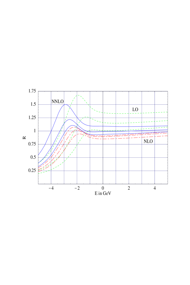
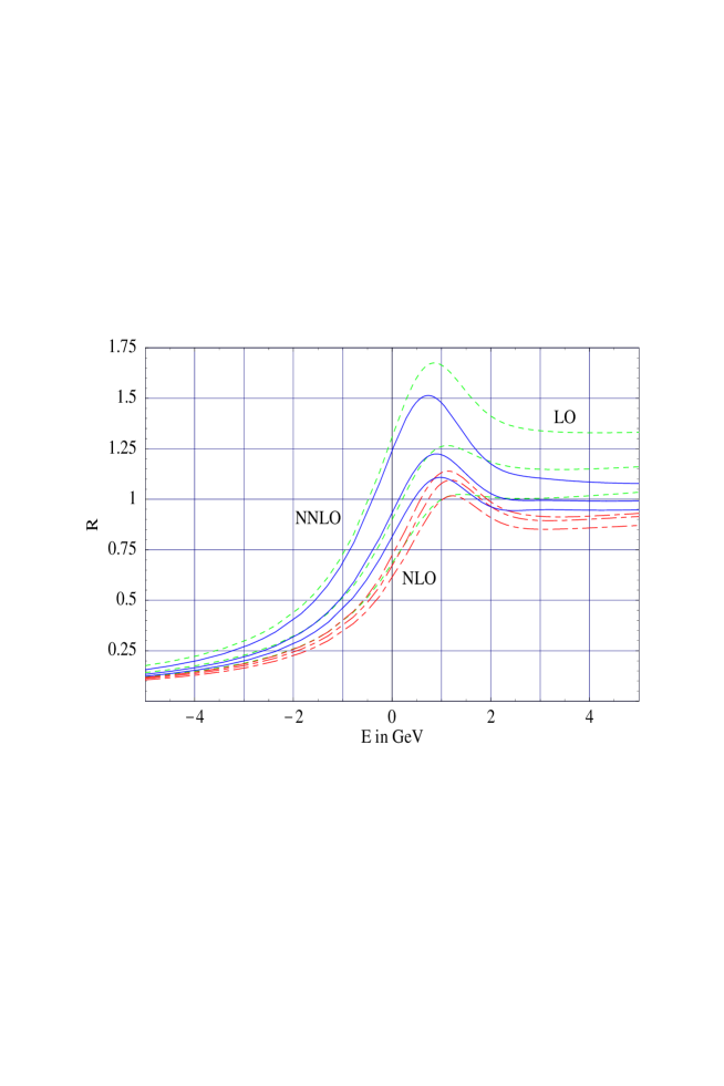
Figure 1: (a) [upper panel]: The normalized $\bar{t}t$ cross section (virtual photon contribution only) in LO (short-dashed), NLO (short-long-dashed) and NNLO (solid) as function of $E=\sqrt{s}-2m_{t}$ (pole mass scheme). Parameters: $m_{t}=\mu_{h}=175\,$GeV, $\Gamma_{t}=1.40\,$GeV, $\alpha_{s}(m_{Z})=0.118$. The three curves for each case refer to $\mu=\left\{15(\mbox{upper});30(\mbox{central});60(\mbox{lower})\right\}\,$GeV. (b) [lower panel]: As in (a), but in the PS mass scheme with $\mu_{f}=20\,$GeV. Hence $E=\sqrt{s}-2m_{t,\rm PS}(20\,\mbox{GeV})$. Other parameters as above with $m_{t}\to m_{t,\rm PS}(20\,\mbox{GeV})$.

The significant shift in the location of the peak impacts directly on the top quark mass measurement. There is no unique choice of the concept of the top quark mass. The top quark pole mass definition has been universally assumed in previous cross section calculations near the threshold; this is indeed an intuitively plausible choice as top quarks do not hadronize. However, the top quark pole mass definition is known to be more sensitive to non-perturbative effects [23] than other mass definitions and the finite width of the top makes no difference in this respect. (The difference is, that the top quark pole mass is irrelevant, because a top quark is always off-shell by an amount $\sqrt{m_{t}\Gamma_{t}}$.). In [13] we argued that the shift of the peak position is related to large perturbative corrections which appear only, when the cross section is expressed in terms of the pole mass, and which have their origin in the sensitivity to distances larger than the toponium Bohr radius. The point is that the Coulomb potential in coordinate space and the pole mass receive the same large corrections [13, 24]. We therefore perform a subtraction on the potential such that the subtracted terms are absorbed into a mass redefinition and at the same time cancel the large corrections to the pole mass. This leads to the ‘potential subtraction (PS) scheme’ and the corresponding mass definition. For further details of the argument we refer to [13]. The PS mass at the subtraction scale $\mu_{f}$ is defined by

$$m_{t,\rm PS}(\mu_{f})=m_{t}-\delta m_{t}(\mu_{f}),$$ (16)

where

$$\delta m_{t}(\mu_{f}) = -\frac{1}{2}\int\limits_{|\vec{q}\,|<\mu_{f}}\!\!\!\frac{d^{3}\mbox{\boldmath${q}$}}{(2\pi)^{3}}\,[\tilde{V}(q)]_{\rm Coulomb}=\Delta(\mu_{f})\Bigg{[}1+\frac{\alpha_{s}}{4\pi}\left(a_{1}-b_{0}\left(\ln\frac{\mu_{f}^{2}}{\mu^{2}}-2\right)\right)$$ (17)

$$+\,\frac{\alpha_{s}^{2}}{(4\pi)^{2}}\Bigg{(}a_{2}-\left\{2a_{1}b_{0}+b_{1}\right\}\left(\ln\frac{\mu_{f}^{2}}{\mu^{2}}-2\right)+b_{0}^{2}\left(\ln^{2}\frac{\mu_{f}^{2}}{\mu^{2}}-4\ln\frac{\mu_{f}^{2}}{\mu^{2}}+8\right)\Bigg{)}\Bigg{]},$$

and $\Delta(\mu_{f})=C_{F}\alpha_{s}\mu_{f}/\pi$. In the following, we re-express the $t\bar{t}$ cross section in terms of the PS mass. We suppose that $\mu_{f}$ scales as $m_{t}\alpha_{s}$ and count $\Delta(\mu_{f})$ as order $m_{t}v^{2}$. Then all terms are re-expanded and terms beyond NNLO are dropped (modulo the resummation near the bound state poles discussed above). Note that $\Delta(\mu_{f})$ is not expanded when it occurs in the combination $\sqrt{s}-2(m_{t,\rm PS}(\mu_{f})+\Delta(\mu_{f}))$. It should also not dominate this combination and this is why we do not use the $\overline{\rm MS}$ mass directly, which would lead to $\Delta\sim m_{t}\alpha_{s}$.

The peak in the $t\bar{t}$ cross section profile is, roughly speaking, the remnant of the first bound state pole (the ‘1S pole’). To understand the effect of the mass redefinition on the cross section qualitatively, it is useful to compute the correction to the 1S pole in terms of both mass definitions. The dominant correction in the pole mass scheme is related to the running coupling in the LO Coulomb potential. So let us take

$$\delta\tilde{V}_{k}(\mbox{\boldmath${q}$})=\frac{-4\pi C_{F}\alpha_{s}}{\mbox{\boldmath${q}$}^{2}}\left(-\frac{b_{0}\alpha_{s}}{4\pi}\ln\frac{\mbox{\boldmath${q}$}^{2}}{\mu^{2}}\right)^{\!k}$$ (18)

to compute the energy level shift

$$\delta E_{k} = \int\!\frac{d^{3}\mbox{\boldmath${q}$}}{(2\pi)^{3}}\frac{d^{3}\mbox{\boldmath${p}$}}{(2\pi)^{3}}\Psi_{\rm 1S}^{*}(\mbox{\boldmath${p}$}+\mbox{\boldmath${q}$}/2)\,\delta\tilde{V}_{k}(\mbox{\boldmath${q}$})\,\Psi_{\rm 1S}(\mbox{\boldmath${p}$}-\mbox{\boldmath${q}$}/2)$$ (19)

$$= \int\!\frac{d^{3}\mbox{\boldmath${q}$}}{(2\pi)^{3}}\left(1+\frac{\mbox{\boldmath${q}$}^{2}}{(m_{t}C_{F}\alpha_{s})^{2}}\right)^{\!-2}\,\delta\tilde{V}_{k}(\mbox{\boldmath${q}$}).$$

The mass of the 1S bound state, including only the leading order Coulomb interaction and the above perturbation, is given by

$$M_{\rm 1S}=2m_{t}+E_{1}^{\rm LO}+\delta E_{k}=2m_{t,\rm PS}(\mu_{f})+E_{1}^{\rm LO,PS}(\mu_{f})+\left[\delta E_{k}+2\delta m_{t}(\mu_{f})\right].$$ (20)

Comparing (19) with (17), we see that the integrands in $\delta E_{k}+2\delta m_{t}(\mu_{f})$ cancel each other for $|\mbox{\boldmath${q}$}|<m_{t}C_{F}\alpha_{s}$ and $|\mbox{\boldmath${q}$}|<\mu_{f}$. At the same time the integral (19) is dominated by the contribution from small ${q}$ quickly as $k$ increases. The result of this exercise for $\mu=30\,$GeV (in which case $m_{t}C_{F}\alpha_{s}(\mu)$ is also about $30\,$GeV) and $\mu_{f}=20\,$GeV is shown in the following table:

$$\begin{array}[]{c|c|c|c|c|c|c|c|c}\hline\cr\hline\cr k&1&2&3&4&5&6&7&8\\ \hline\cr\delta E_{k}/\mbox{MeV}&-489&-214&-109&-78&-67&-70&-85&-118\\ \hline\cr(\delta E_{k}+2\delta m_{t})/\mbox{MeV}&+97&+0.8&+3.5&+0.1&+0.3&0&0&0\\ \hline\cr\hline\cr\end{array}\vspace*{-0.2cm}$$

This shows that the prediction for the mass of the 1S state is stable in terms of the PS mass, and we expect a qualitatively similar conclusion for the top quark cross section. (The same observation can also be used to determine the bottom quark $\overline{\rm MS}$ mass from the $\Upsilon$ resonances accurately [25].) To demonstrate that the PS mass can also be related more accurately to the $\overline{\rm MS}$ mass $\bar{m}_{t}=m^{\overline{\rm MS}}_{t}(m^{\overline{\rm MS}})$, we assume $\bar{m}_{t}=165\,$GeV and obtain, adding loop corrections consecutively,

$$m_{t} = \left[165.0+7.6+1.6+0.6\,(\mbox{est.})\right]\,\mbox{GeV}$$ (21)

$$m_{t,\rm PS}(20\,\mbox{GeV}) = \left[165.0+6.7+1.2+0.3\,(\mbox{est.})\right]\,\mbox{GeV}.$$ (22)

The 2-loop correction follows from [26] and (17) and the 3-loop correction is based on an estimate in the so-called ‘large-$\beta_{0}$-limit’ [27]. Hence, the present uncertainty in the relation of the PS mass to the $\overline{\rm MS}$ mass is about $300\,$MeV.

4. Discussion. The $t\bar{t}$ cross section expressed in terms of $m_{t,\rm PS}(\mu_{f})$ with $\mu_{f}=20\,$GeV is shown in the lower panel of Fig. 1. Since the horizontal scale $E$ is now defined as $\sqrt{s}-2m_{t,\rm PS}(20\,\mbox{GeV})$, we observe an overall, but trivial shift, related to the fact that $m_{t}-m_{t,\rm PS}(20\,\mbox{GeV})=1.75\,$GeV for $\mu=30\,$GeV. The important change is that in the PS scheme the location of the peak moves little as we go from LO to NLO to NNLO. Furthermore, the scale dependence of the peak location under variations of $\mu$ between $15$ and $60\,$ GeV is reduced by a factor of 2. The transition from the pole to the PS scheme has little effect on the shape and overall normalization of the cross section as expected. In particular a significant uncertainty of about $\pm 20\%$ in the normalization remains, larger than at NLO.

The strong enhancement of the peak for the small scale $\mu=15\,$GeV is a consequence of the fact that the perturbative corrections to the residue of the 1S pole (see (S0.Ex9)) become uncontrollable at scales not much smaller than $15\,$GeV. We find that these large corrections are mainly associated with the logarithms that make the coupling run in the Coulomb potential. This could be interpreted either as an indication that higher order corrections are still important (at such low scales) or that the terms associated with $b_{0}$ should be treated exactly, because they are numerically (but not parametrically) large. (If the Schrödinger equation with the potential (10) is solved exactly by numerical methods, the scale dependence of the peak height is indeed smaller [28].) Inspecting the logarithms in the result for the cross section, choosing an energy-dependent scale $\mu=2\,(m_{t}\,(E^{2}+\Gamma_{t}^{2})^{1/2})^{1/2}$ would be most appropriate. Although this choice is our preferred one, we refrained from using it for the comparison of the pole and PS scheme, since the peak positions are at different energies in the two schemes.

The uncertainties due to other parameters turn out to be less than the uncertainty due to the variation of the scale $\mu$. The dependence on $\alpha_{s}(m_{Z})$ is discussed below. Varying $\mu_{h}$ by a factor of two around $m_{t}$ changes the cross section by a few percent near the peak. The effect of summing logarithms to NLL is of the same order. We have also checked the effect of some NNLL logarithms on the calculation and find a variation of the order of $\pm 5\%$. The relatively small effect of renormalization group improvement is a consequence of the absence of leading logarithms. We also checked the effect of varying $\mu_{f}$ between 5 and $40\,$GeV. From a purely pragmatic point of view, values of $\mu_{f}$ around $40\,$GeV lead to the most stable result. However, since $\mu_{f}<m_{t}C_{F}\alpha_{s}(\mu)\approx 30\,$ GeV is required from a conceptual point of view, we have chosen $\mu_{f}=20\,$GeV as our preferred setting. (From the point of view of non-perturbative infrared cancellations, it would be sufficient to choose $\mu_{f}$ larger than the strong interaction scale $1\,$GeV. However, from (19) we see that the cancellation becomes effective – and the perturbative correction universal – as soon as the integrand is dominated by $|\mbox{\boldmath${q}$}|<m_{t}C_{F}\alpha_{s}$. For this reason it is legitimate and advantageous to choose $\mu_{f}$ significantly larger than the strong interaction scale.)

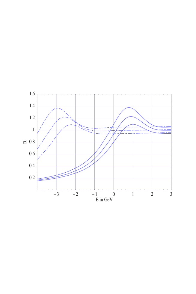
Figure 2: Dependence of the NNLO $t\bar{t}$ cross section on $\alpha_{s}(m_{Z})$ in the PS scheme (solid) and the pole scheme (long-short-dashed). The three curves in each scheme refer to $\alpha_{s}(m_{Z})=0.113$ (lower), $\alpha_{s}(m_{Z})=0.118$ (middle) and $\alpha_{s}(m_{Z})=0.123$ (upper). Recall that $E=\sqrt{s}-2m_{t}$ in the pole scheme but $E=\sqrt{s}-2m_{t,\rm PS}(20\,\mbox{GeV})$ in the PS scheme. Other parameters: $m_{t}=\mu_{h}=175\,$GeV, $\Gamma_{t}=1.40\,$GeV, $\mu=30\,$GeV.

If we take (naively) the change in the peak position under scale variations as a measure of the uncertainty of the top mass measurement, we conclude that a determination of the PS mass with an error of about $100\,$-$150\,$MeV is possible. Given that the uncertainty in relating the PS mass to the $\overline{\rm MS}$ mass is about $300\,$MeV, this accuracy seems to be sufficient. We emphasize that it is not sufficient to invent an ad hoc mass definition in terms of which the peak position is stable empirically. In addition, such a mass definition needs to have a well-behaved relation order by order in perturbation theory to a mass definition relevant to top quark processes far away from threshold. For a realistic assessment of the error in the mass measurement, the theoretical line shape has to be folded with initial state radiation, beamstrahlung and beam energy spread effects. Since these effects are well understood, the main question that needs to be addressed is whether the normalization uncertainty leads to a degradation of the mass measurement after these sources of smearing are taken into account. This should be studied in a collider design specific setting.

In the PS scheme the correlation of the top quark mass with $\alpha_{s}$ is also strongly reduced, mainly because the perturbative corrections to the 1S pole are small in this scheme. This is indicated by Fig. 2, which shows the dependence of the line shape on the value of $\alpha_{s}(m_{Z})$. One can therefore rely less on input from top quark momentum distributions, which have been used in the pole scheme to constrain $m_{t}$ and $\alpha_{s}(m_{Z})$ simultaneously. Since momentum distributions are more sensitive to non-perturbative effects than the inclusive cross section, this is another advantage of the PS scheme.

In conclusion, we evaluated the next-to-next-to-leading order QCD correction to top quark production near threshold in the conventional pole scheme and in the PS scheme [13]. We employed factorization in dimensional regularization and summed next-to-leading logarithms in the top quark velocity. We find that the cross section expressed in the PS scheme allows us to determine the top PS mass more accurately than the top pole mass. The PS mass, in turn, can also be related more accurately to the top quark $\overline{\rm MS}$ mass.

Acknowledgements. We thank A.H. Hoang for extensive discussions and for comparing numerical results of their calculation [28] prior to publication. The work of M.B. is supported in part by the EU Fourth Framework Programme ‘Training and Mobility of Researchers’, Network ‘Quantum Chromodynamics and the Deep Structure of Elementary Particles’, contract FMRX-CT98-0194 (DG 12 - MIHT). The work of V.S. has been supported by the Volkswagen Foundation, contract No. I/73611, the Russian Foundation for Basic Research, project 98–02–16981 and by INTAS, grant 93–0744.

References

- [1] CDF collaboration (F. Abe et al.), Phys. Rev. Lett. 80 (1998) 2767; CDF collaboration (F. Abe et al.), FERMILAB-PUB-98-319-E [hep-ex/9810029]; D0 Collaboration (B. Abbott et al.), Phys. Rev. D58 (1998) 052001.
- [2] ECFA/DESY LC Physics Working Group (E. Accomando et al.), Phys. Rep. 299 (1998) 1.
- [3] V.S. Fadin and V.A. Khoze, Pis’ma Zh. Eksp. Teor. Fiz. 46, 417 (1987) [JETP Lett. 46, 525 (1987)]; Yad. Fiz. 48, 487 (1988) [Sov. J. Nucl. Phys. 48(2), 309 (1988)].
- [4] M.J. Strassler and M.E. Peskin, Phys. Rev. D43 (1991) 1500; W. Kwong, Phys. Rev. D43 (1991) 1488; M. Jezabek, J.H. Kühn and T. Teubner, Z. Phys. C56 (1992) 653; M. Jezabek and T. Teubner, Z. Phys. C59 (1993) 669; Y. Sumino, K. Fujii, K. Hagiwara, H. Murayama and C.-K. Ng, Phys. Rev. D47 (1993) 56; K. Fujii, T. Matsui and Y. Sumino, Phys. Rev. D50 (1994) 4341; R. Harlander, M. Jezabek, J.H. Kühn and T. Teubner, Phys. Lett. B346 (1995) 137; M. Jezabek et al., Phys. Rev. D58 (1998) 014006.
- [5] I.I. Bigi et al., Phys. Lett. B181 (1986) 157.
- [6] Y. Schröder, [hep-ph/9812205].
- [7] M. Peter, Phys. Rev. Lett. 78 (1997) 602; Nucl. Phys. B501 (1997) 471.
- [8] M. Beneke, A. Signer and V.A. Smirnov, Phys. Rev. Lett. 80 (1998) 2535.
- [9] A. Czarnecki and K. Melnikov, Phys. Rev. Lett. 80 (1998) 2531.
- [10] A.H. Hoang and T. Teubner, Phys. Rev. D58 (1998) 114023.
- [11] K. Melnikov and A. Yelkhovsky, Nucl. Phys. B528 (1998) 59.
- [12] O. Yakovlev, [hep-ph/9808463].
- [13] M. Beneke, Phys. Lett. B434 (1998) 115.
- [14] M. Beneke, A. Signer and V.A. Smirnov, in preparation.
- [15] K. Melnikov and O. Yakovlev, Phys. Lett. B324 (1994) 217; V.S. Fadin, V.A. Khoze and A.D. Martin, Phys. Rev. D49 (1994) 2247; W. Beenakker, F.A. Berends, A.P. Chapovsky, [hep-ph/9902304].
- [16] M. Beneke and V.A. Smirnov, Nucl. Phys. B522 (1998) 321.
- [17] R. Barbieri, R. Gatto, R. Körgerler and Z. Kunszt, Phys. Lett. 57B (1975) 455.
- [18] A. Pineda and J. Soto, Nucl. Phys. Proc. Suppl. 64 (1998) 428 [hep-ph/9707481]; Phys. Rev. D59 (1999) 016005.
- [19] L. Susskind, Les Houches lectures 1976, in: Weak and electromagnetic interactions at high energies, R. Balian et al. (eds.) (North-Holland, Amsterdam, 1977); W. Fischler, Nucl. Phys. B129 (1977) 157; A. Billoire, Phys. Lett. B92 (1980) 343.
- [20] A. Pineda and F.J. Yndurain, Phys. Rev. D58 (1998) 094022.
- [21] K. Melnikov and A. Yelkhovsky, TTP98-17 [hep-ph/9805270].
- [22] A.A. Penin and A.A. Pivovarov, INR-0991-98 [hep-ph/9810496].
- [23] M. Beneke and V.M. Braun, Nucl. Phys. B426 (1994) 301; I.I. Bigi, M.A. Shifman, N.G. Uraltsev and A.I. Vainshtein, Phys. Rev. D50 (1994) 2234; M. Beneke, Phys. Lett. B344 (1995) 341; M.C. Smith and S.S. Willenbrock, Phys. Rev. Lett. 79 (1997) 3825.
- [24] A.H. Hoang, M.C. Smith, T. Stelzer and S. Willenbrock, UCSD/PTH 98-13 [hep-ph/9804227].
- [25] M. Beneke, A. Signer and V.A. Smirnov, in: Proceedings of RADCOR98, Barcelona, September 1998.
- [26] N. Gray, D.J. Broadhurst, W. Grafe and K. Schilcher, Z. Phys. C48 (1990) 673.
- [27] M. Beneke and V.M. Braun, Phys. Lett. 348 (1995) 513; P. Ball, M. Beneke and V.M. Braun, Nucl. Phys. B452 (1995) 563.
- [28] A.H. Hoang and T. Teubner, in preparation.