Neutrino oscillations and mixings with three flavors

Abstract

Global fits to all data of candidates for neutrino oscillations are presented in the framework of a three-flavor model. The analysis excludes mass regions where the MSW effect is important for the solar neutrino problem. The best fit gives $\theta_{1}\approx 28.9^{\circ}$, $\theta_{2}\approx 4.2^{\circ}$, $\theta_{3}\approx 45.0^{\circ}$, $m_{2}^{2}-m_{1}^{2}\approx 2.87\times 10^{-4}\;{\rm eV}^{2}$, and $m_{3}^{2}-m_{2}^{2}\approx 1.11\;{\rm eV}^{2}$ indicating essentially maximal mixing between the two lightest neutrino mass eigenstates.

I Introduction

Neutrino oscillations were reported last year by the Super-Kamiokande Collaboration [1] to have been convincingly seen by the Super-Kamiokande detector in Kamioka, Japan, in the study of the atmospheric neutrino problem. This has rekindled interest to explain also other deviations from expected results in neutrino physics in terms of neutrino oscillations. There are at present essentially four different types of experiments looking for neutrino oscillations: solar neutrino experiments, atmospheric neutrino experiments, accelerator neutrino experiments, and reactor neutrino experiments.

Most analyses of neutrino data so far have been performed in two-flavor models. Although this is quite illustrative, it can lead to wrong conclusions concerning the necessary number of degrees of freedom to explain data. It is, e.g., possible that the four neutrino scenario, advocated by several authors, is an artifact of this simplification.

Recently, several papers [2, 3, 4, 5, 6, 7, 8, 9] have been published pertaining at demonstrating the possibility to obtain an overall description in terms of a three-flavor model. Most of these investigations have focused on demonstrating the plausibility of the scenario, without truly fitting all the data.

Here we would like to report on the first stage of a global analysis of all the neutrino oscillation data in a three-flavor model. We will assume that $CP$ nonconservation is negligible at the present level of experimental accuracy. Thus, the Cabibbo-Kobayashi-Maskawa (CKM) mixing matrix for the neutrinos is real. There are then in principle five parameters that can be fitted in this model: Three mixing angles and two mass squared differences. (This is in contrast with two two-flavor models, which give only four parameters: Two mixing angles and two mass squared differences.) The two mass squared differences in the three-flavor model enter the argument of the sinodial function in combination with the ratio $L/E$, where $L$ is the source-detector distance and $E$ is the neutrino energy. The argument of the sinodial functions related to the energy dependence can then be treated as yet another angle. In this case, the probability function can be seen as given by a rotation of the flavor states by five angles. This is in analogy to the two-flavor case, which can be seen as a rotation by two angles, one of which is given by $\Delta m^{2}L/4E$, $\Delta m^{2}$ being the mass squared difference of the two neutrino masses.

In the present analysis, we will make the simplifying assumption that the relevant ranges of mass squared differences are such that the Mikheyev-Smirnov-Wolfenstein (MSW) effect [10] in the Sun is negligible. This excludes essentially the sensitivity region $10^{-6}$–$10^{-5}$ eV². The absence of any day-night variation in the Super-Kamiokande and Kamiokande data is also consistent with neglecting the MSW resonance effect in the Earth for the electron-neutrino data.

The differing results for the solar neutrino experiments present another problem. Since the Super-Kamiokande and Kamiokande experiments can resolve the energy for the solar neutrinos, these experiments are of a rather different and more detailed kind than the radio-chemical experiments. It is possible to vary the disappearance rate by going to a mass squared realm, where the arguments, i.e., the angles that depend on the mass squared differences, are sensitive to the energy of the neutrinos, since this is different for the different detection methods. However, in this case, the energy domains for the different experiments do not vary in the way expected, making the Cl experiment the smallest ($\approx 0.33$) and the Ga experiments the largest ($\approx 0.6$) of the expected rate. One would, in fact, expect the Super-Kamiokande experiment, with the highest mean energy for the neutrinos, to give the smallest result, whereas in reality it is in between.

Confronting this with the apparent lack of variation in the experimental solar neutrino detection probability with energy, at least up to approximately 13 MeV, in the Super-Kamiokande data, we will adopt the point of view that the mass squared differences are in a range that leads to the solar neutrino oscillations being averaged out to their classical values. By fitting the three mixing angles, we then account for the weighted mean of all the solar neutrino experiments. By nature of the sensitivity level of the accelerator and atmospheric neutrino experiments, we will choose the mass squared difference ranges as $0.2\;{\rm eV^{2}}\leq\Delta M^{2}\leq 2\;{\rm eV^{2}}$ and $10^{-4}\;{\rm eV^{2}}\leq\Delta m^{2}\leq 10^{-3}$ eV². Here $\Delta M^{2}$ will regulate the accelerator experiments and the multi-GeV atmospheric neutrino data, whereas $\Delta m^{2}$ regulates the low energy atmospheric experiments. This choice is thus not inherited from two-flavor model analyses, but arises from the sensitivity of the different types of experiments.

It is in principle possible that there would be a resonance effect for the atmospheric electron-neutrinos passing through Earth. Our chosen ranges for the mass squared differences exclude this effect in the present fit, since $\Delta m^{2}\geq 10^{-4}$ eV².

Since the reactor experiments are disappearance experiments with no signal seen, they can at best exclude certain ranges for the mass squared differences due to their sensitivity level. The two ranges of mass squared differences chosen here respect this sensitivity level.

The paper is organized as follows. In Sec. II, we briefly discuss the formalism used in our analysis including notations, Gaussian averaging, and minimization. In Sec. III, we discuss the choice of data from different experiments used in the minimization procedure. Sec. IV describes the minimization procedure and includes the results thereof. We also show that our results are consistent with the experimental data, assuming that all of the deviations from the expected values are indeed related to the physics of neutrino oscillations. Finally, Sec. V presents a discussion of the results and also our main conclusions.

II Formalism

A Notations

In the present analysis, we will use the plane-wave approximation to describe neutrino oscillations. In this approximation, a neutrino state $|\nu_{\alpha}\rangle$ with flavor $\alpha$ is a linear combination of neutrino mass eigenstates $|\nu_{a}\rangle$ such that

$$|\nu_{\alpha}\rangle=\sum_{a=1}^{3}U_{\alpha a}^{\ast}|\nu_{a}\rangle,\quad\alpha=e,\mu,\tau,$$ (1)

where the $U_{\alpha a}$’s are entries in a unitary $3\times 3$ matrix $U$.

The unitary matrix $U$ is given by

$$U=(U_{\alpha a})=\left(\begin{array}[]{ccc}U_{e1}&U_{e2}&U_{e3}\\ U_{\mu 1}&U_{\mu 2}&U_{\mu 3}\\ U_{\tau 1}&U_{\tau 2}&U_{\tau 3}\end{array}\right).$$ (2)

A convenient parametrization for $U$ is [11]

$$U=\left(\begin{array}[]{ccc}c_{2}c_{3}&s_{3}c_{2}&s_{2}\\ -s_{3}c_{1}-s_{1}c_{3}s_{2}&c_{1}c_{3}-s_{1}s_{2}s_{3}&s_{1}c_{2}\\ s_{1}s_{3}-s_{2}c_{1}c_{3}&-s_{1}c_{3}-s_{2}s_{3}c_{1}&c_{1}c_{2}\end{array}\right),$$ (3)

where $s_{i}\equiv\sin\theta_{i}$ and $c_{i}\equiv\cos\theta_{i}$ for $i=1,2,3$. This is the so called standard representation of the CKM mixing matrix. We have here put the $CP$ phase equal to zero in the CKM matrix. This means that $U^{\ast}_{\alpha a}=U_{\alpha a}$ for $\alpha=e,\mu,\tau$ and $a=1,2,3$.

The probability of transition from a neutrino flavor state $\alpha$ to a neutrino flavor state $\beta$ is given by

$$P_{\alpha\beta} \equiv P(\nu_{\alpha}\to\nu_{\beta})$$ (4)

$$= \delta_{\alpha\beta}-4\;\underset{a<b}{\sum_{a=1}^{3}\sum_{b=1}^{3}}U_{\alpha a}U_{\beta a}U_{\alpha b}U_{\beta b}$$ (5)

$$\times \sin^{2}\frac{\Delta m_{ab}^{2}L}{4E},\quad\alpha,\beta=e,\mu,\tau,$$ (6)

where $\delta_{\alpha\beta}$ is Kronecker’s delta and $\Delta m_{ab}^{2}\equiv m_{a}^{2}-m_{b}^{2}$. The three mass squared differences $\Delta m_{21}^{2}$, $\Delta m_{32}^{2}$, and $\Delta m_{13}^{2}$ are not linearly independent, since they satisfy the relation

$$\Delta m_{21}^{2}+\Delta m_{32}^{2}+\Delta m_{13}^{2}=0.$$ (7)

Therefore, we will define

$$\Delta m^{2} \equiv \Delta m_{21}^{2}=m_{2}^{2}-m_{1}^{2},$$ (8)

$$\Delta M^{2} \equiv \Delta m_{32}^{2}=m_{3}^{2}-m_{2}^{2},$$ (9)

and thus $\Delta m_{31}^{2}=-\Delta m_{13}^{2}=\Delta m^{2}+\Delta M^{2}$.

From Eq. (6) it is clear that $P({\bar{\nu}}_{\beta}\to{\bar{\nu}}_{\alpha})=P(\nu_{\alpha}\to\nu_{\beta})$ and since we have assumed that $CP$ is conserved, i.e., the CKM mixing matrix $U$ is real, it holds that $P(\nu_{\beta}\to\nu_{\alpha})=P(\nu_{\alpha}\to\nu_{\beta})$. This implies that

$$P({\bar{\nu}}_{\alpha}\to{\bar{\nu}}_{\beta})=P(\nu_{\alpha}\to\nu_{\beta}).$$ (10)

B Gaussian averaging

Since in practice the neutrino wave is neither detected nor produced with sharp energy or with well defined propagation length, we have to average over the $L/E$ dependence and other uncertainties in the detection and emission of the neutrino wave. We will here use the Gaussian average, which is defined by

$$\langle P\rangle=\int_{-\infty}^{\infty}P(x)f(x)\,dx,$$ (11)

where

$$f(x)=\frac{1}{\gamma\sqrt{2\pi}}e^{-(x-l)^{2}/2\gamma^{2}}.$$

Here $l$ and $\gamma$ are the expectation value and standard deviation, respectively.

By taking the Gaussian average of Eq. (6), we obtain the average transition probabilities from flavor $\nu_{\alpha}$ to flavor $\nu_{\beta}$ as

$$\langle P_{\alpha\beta}\rangle = \delta_{\alpha\beta}-2\;\underset{a<b}{\sum_{a=1}^{3}\sum_{b=1}^{3}}U_{\alpha a}U_{\beta a}U_{\alpha b}U_{\beta b}$$ (12)

$$\times \left[1-\cos\left(2l\Delta m_{ab}^{2}\right)e^{-2\gamma^{2}(\Delta m_{ab}^{2})^{2}}\right],$$ (14)

$$\alpha,\beta=e,\mu,\tau.$$

The physical interpretations of the parameters $l$ and $\gamma$ are the following: The parameter $l$ deals with the sensitivity of an experiment and is given by $l\simeq 1.27\langle L/E\rangle$, where $\langle L/E\rangle$ should be given in km/GeV or m/MeV, and $\Delta m_{ab}^{2}$ should be measured in ${\rm eV}^{2}$. Note that we will here use $\langle L/E\rangle=\langle L\rangle/\langle E\rangle$. The parameter $\gamma$ is a so called damping factor. For large values of $\gamma$, the dependence on the mass squared differences will be completely washed out, since $1-\cos\left(2l\Delta m_{ab}^{2}\right)e^{-2\gamma^{2}(\Delta m_{ab}^{2})^{2}}\to 1$ when $\gamma\to\infty$, and the transition probabilities $\langle P_{\alpha\beta}\rangle$ will just be dependent on the mixing angles $\theta_{i}$, where $i=1,2,3$. This corresponds to the classical limit. In the other limit, $\gamma\to 0$, we will just regain Eq. (6) from Eq. (14), i.e., $\lim_{\gamma\to 0}\langle P_{\alpha\beta}\rangle=P_{\alpha\beta}$.

C Minimization

In order to obtain the mixing angles $\theta_{i}$, where $i=1,2,3$, and the mass squared differences $\Delta m^{2}$ and $\Delta M^{2}$, we minimize the following object function

$$F \equiv F(\theta_{1},\theta_{2},\theta_{3},\Delta m^{2},\Delta M^{2})$$ (15)

$$= \frac{1}{w}\sum_{i=1}^{N_{\rm exp}}w_{i}\frac{1}{{P^{\rm exp}_{i}}^{2}}\left(P_{i}-P^{\rm exp}_{i}\right)^{2},$$ (16)

where $w=\sum_{i=1}^{N_{\rm exp}}w_{i}$ and $N_{\rm exp}$ is the number of neutrino oscillation experiments. The function $F$ is a least square method error function for the relative errors of the neutrino oscillation experiments with weights $w_{i}\geq 0$, where $i=1,2,\ldots,N_{\rm exp}$. The quantities $P_{i}=\langle P_{\alpha\beta}\rangle_{i}$ and $P^{\rm exp}_{i}$ are the theoretical (model) and experimental transition probabilities for the $i$th experiment, respectively. The reason why we are using relative errors in the error function and not absolute errors (as is usually done) is due to the fact that the different categories of experiments have rather different numerical ranges for the experimental transition probabilities. In the rest of this paper, we will write $P_{\alpha\beta}$, $L$, and $E$ instead of $\langle P_{\alpha\beta}\rangle$, $\langle L\rangle$, and $\langle E\rangle$, respectively, to keep the notations simpler.

In accordance with the discussion in the Introduction, the following constraints will be used in the minimization procedure

$$0\leq\theta_{i}\leq\frac{\pi}{2},\quad\mbox{where $i=1,2,3,$}$$ (17)

$$10^{-4}\;{\rm eV}^{2}\leq\Delta m^{2}\leq 10^{-3}\;{\rm eV}^{2},$$ (18)

$$0.2\;{\rm eV}^{2}\leq\Delta M^{2}\leq 2\;{\rm eV}^{2}.$$ (19)

The weights in the object function (16) will be chosen as

$$w_{i}\sim\frac{1}{n\epsilon_{i}},$$ (20)

where $n$ is the number of experiments used in the minimization of the same category (solar, atmospheric, accelerator, or reactor) and $\epsilon_{i}=\Delta P_{i}/P^{\rm exp}_{i}$ is the relative error in the $i$th experiment.

Our choice for the weights is motivated by our wish to treat all categories of experiments on the same footing (the factor $1/n$), and enhance experiments with small relative errors (the factor $1/\epsilon_{i}$). Here again, relative errors are used, since the range of values of the probabilities are rather different. However, in all our cases, $\epsilon_{i}<1$. Higher powers of $1/\epsilon_{i}$ would enhance the good experiments too much. Since $\Delta P_{i}$ is a sum of the statistical and systematical errors, an underestimation of the latter will, of course, also overemphasize the relative weight of a certain experiment.

For the damping factor of an experiment, we will use

$$\gamma\sim\frac{L}{E}\left(\frac{\Delta L}{L}+\frac{\Delta E}{E}\right),$$ (21)

where $\Delta L$ is a combination of the uncertainties coming from (a) the length of the detector and (b) the distance between the detector and the neutrino source and $\Delta E$ is the uncertainty in the mean neutrino energy. In Table I, we have listed all the experiments, which we have used in the minimization procedure.

III Choice of Data

Most of the data used in our analysis are taken directly from the quoted publications. (See Table I for the references to each experiment.) We have chosen in this first analysis not to discriminate between the various experiments in any other way than by their experimental uncertainties.

A Solar neutrino experiments

For the chlorine (Cl) and gallium (Ga) experiments, we will define the mean neutrino energy as

$$E=\frac{1}{S}\sum_{r}\langle E\rangle_{r}S^{(r)},$$ (22)

where $S=\sum_{r}S^{(r)}$. The index $r$ labels the different solar neutrino sources. In the case of a Cl experiment (Homestake), $r$ can be pep, ⁷Be, ⁸B, hep, ¹⁵O, or ¹⁷F, and similarly for a Ga experiment (SAGE or GALLEX), $r$ can be pp, pep, ⁷Be, ⁸B, hep, ¹³N, ¹⁵O, or ¹⁷F. The quantities $\langle E\rangle_{r}$ and $S^{(r)}$ are the average neutrino energy and standard solar model (SSM) prediction for the neutrino capture rates of the solar neutrino source $r$, respectively. Using the values given by the Bahcall-Basu-Pinsonneault 1998 (BBP98) SSM [12, 13], we obtain the mean neutrino energy to be $E_{\rm Ga}\approx 1.1\;{\rm MeV}$ for the SAGE and GALLEX experiments and $E_{\rm Cl}\approx 5.5\;{\rm MeV}$ for the Homestake experiment.

As for the water-Cherenkov detector experiments (Super-Kamiokande and Kamiokande), we have chosen the mean energy of the neutrinos to be $E_{\rm w-C}\approx 10\;{\rm MeV}$. We will assume that the uncertainty in the energy is $\Delta E\sim E$, respecting the threshold energy for detection. For the Super-Kamiokande and Kamiokande experiments, the energy resolution is taken to be $\Delta E\sim 2$ MeV.

For solar neutrino experiments, the path length for the neutrinos is given by the mean Sun-Earth distance. The length of the detector, the deviation in the Earth’s orbit around the Sun, and the solar radius are all small in this connection, giving $\Delta L/L\sim 0$ for solar neutrinos.

B Atmospheric neutrino experiments

The path length of the atmospheric neutrinos is given by

$$L\equiv L(\vartheta)=\sqrt{R^{2}\cos^{2}\vartheta+2Rd+d^{2}}-R\cos\vartheta,$$ (23)

where $\vartheta$ is the so called zenith angle, $R$ is the radius of the Earth, and $d$ is the altitude of the production point of atmospheric neutrinos. We have taken $R\approx 6400\;{\rm km}$ and $d\approx 10\;{\rm km}$, which gives $L\approx 1.22\times 10^{4}\;{\rm km}$ for the bin mean value $\cos\vartheta=-0.95$ (MACRO and Kamiokande) and $L\approx 1.03\times 10^{4}\;{\rm km}$ for bin mean value $\cos\vartheta=-0.8$ (Soudan, Super-Kamiokande, and IMB). The bins $-1\leq\cos\vartheta\leq-0.9$ and $-1\leq\cos\vartheta\leq-0.6$ have $\Delta L/L\sim 0.10$ and $\Delta L/L\sim 0.50$, respectively.

The atmospheric neutrino experiments present a special problem, since they are not entirely comparable to each other. The Super-Kamiokande experiment measures several parameters and has presented the “ratio of ratios” integrated over the energy (actually $L/E$) as does also the Kamiokande experiment. Other experiments can only measure the ratio of observed neutrino flux and expected neutrino flux. The double ratio eliminates most of the uncertainty in the muon-neutrino flux. However, this function is also more complicated to fit, and has lost much of the information of path length and energy of the neutrinos. We have therefore used the directly measured disappearance rates evaluated from the data for upward-going events given in the tables and figures of Refs. [1, 7, 14, 15, 16, 17]. This makes it possible to use several of the other atmospheric neutrino experiments on the same footing. The disadvantage is the uncertainty in the expected neutrino flux. This uncertainty is claimed to be of the order of $20\%$ [1].

The main uncertainty of the neutrino flux comes from the uncertainty in the primary cosmic radiation flux giving rise to the pions and kaons responsible for the muon and (later) electron neutrinos. Let the overall factor of flux uncertainty be denoted by $\eta_{\alpha}$ for neutrino flavor $\nu_{\alpha}$. Thus, e.g., the actual muon-neutrino flux is $\tilde{\Phi}_{\mu}=\eta_{\mu}\Phi_{\mu}$, where $\Phi_{\mu}$ is the theoretical muon-neutrino flux calculated in Ref. [18]. Then, in the absence of neutrino oscillations, the ratio of measured and theoretical flux is just $R_{\mu}=\eta_{\mu}$. In the presence of neutrino oscillations, on the other hand, we instead obtain

$$R_{\alpha}=\frac{\tilde{\Phi}_{e}P_{e\alpha}+\tilde{\Phi}_{\mu}P_{\mu\alpha}+\tilde{\Phi}_{\tau}P_{\tau\alpha}}{\Phi_{\alpha}},$$ (24)

for any flavor $\alpha=e,\mu,\tau$. Here $P_{\alpha\beta}$ is the probability of oscillation from flavor $\alpha$ to flavor $\beta$. Since the ratio $R=\Phi_{\mu}/\Phi_{e}$ is considered to be quite well determined theoretically, perhaps even to $5\%$, due to known branching ratios of the pions [18] and their decays, we conclude that the various factors $\eta_{\alpha}$ are essentially the same for $\alpha=e,\mu$. This is consistent with the picture, which says that the uncertainty is due to uncertainty in the primary cosmic ray flux. We will further also neglect contributions from the $\tau$ leptons in what follows. They should come from production of $c$ or $b$ mesons, but the relevant cross sections are small compared to the pion cross sections.

For the muon-neutrino ratio measured by several experiments, we obtain

$$R_{\mu}=\eta\left(P_{\mu\mu}+\frac{1}{R}P_{e\mu}\right).$$ (25)

At $E\approx 10$ GeV (Super-Kamiokande), we have $R\simeq 3$ [1, 18], and the last term can be neglected if $P_{e\mu}$ is small, which turns out to be the case. Thus, we obtain $P_{\mu\mu}\simeq\eta^{-1}R_{\mu}$. We will therefore calculate the solution with the overall factor $\eta$ varying from $0.8$ to $1.2$ in the experimental values for $R_{\mu}$ of upward-going events with $\cos\vartheta\leq-0.6$.

For the electron-neutrino ratio $R_{e}=\eta(P_{ee}+RP_{\mu e})$, the term $RP_{\mu e}$ is not negligable compared to the term $P_{ee}$, and can therefore not be neglected. Instead of using $R_{e}$ as input, we will analyze $R_{e}$ as an outcome of the optimization process, i.e., in terms of the fitted parameters.

Finally, the sensitivity for the atmospheric neutrinos can be divided into two groups. The first group (Soudan and Super-Kamiokande) is sensitive to the small mass squared difference only, whereas the second group (MACRO, Kamiokande, and IMB) is sensitive both to the large and (slightly) to the small mass squared differences. Changing the ratio from $0.8$ to $1.2$ times the quoted ones (Table I), will therefore influence the determination of the mass squared differences.

C Accelerator neutrino experiments

The mean energies and path lengths for the accelerator neutrino experiments are all given in Refs. [19, 20, 21, 22]. In most cases, a measure of $\Delta L$ is given by half the length of the detector, giving $\Delta L/L$ in the range $0.15$–$0.35$. For the transition probabilities, we have used the presented $90\%$ C.L. upper bounds, except for the Liquid Scintillator Neutrino Detector (LSND) experiment, for which we have used their quoted $\nu_{\mu}\rightarrow\nu_{e}$ transition probability.

D Reactor neutrino experiments

The reactor neutrino experiments are all disappearance experiments with no signal detected. We have used the published $90\%$ C.L. bounds on disappearance signals mainly to limit the mass squared ranges. Once these are outside the sensitivities of the reactor experiments, the solution will automatically reproduce these. For the reactor experiments, the uncertainties in $L$ are all small compared to the uncertainties in energy determination.

IV Numerical Analysis

To be able to minimize Eq. (16) we have to use numerical methods, since there is no successful way to do this with analytical methods, the present function being to large and we have far too many variables. Our procedure will be as follows. First, we will use a very simple stochastic procedure. We choose some number ($n$) of random points in the specified domain and evaluate the object function (16). We simply take the point which gives the smallest value of this function. To obtain good statistics we repeat this procedure $N$ times. Including all 16 experiments, discussed in the previous section, and choosing $n=10^{6}$ and $N=20$, we obtained

$$\theta_{1}=28.7^{\circ}\pm 0.7^{\circ},$$ (26)

$$\theta_{2}=4.4^{\circ}\pm 0.1^{\circ},$$ (27)

$$\theta_{3}=45.1^{\circ}\pm 0.3^{\circ},$$ (28)

$$\Delta m^{2}=(2.89\pm 0.21)\times 10^{-4}\;{\rm eV}^{2},$$ (29)

$$\Delta M^{2}=1.12\pm 0.04\;{\rm eV}^{2},$$ (30)

where we have used

$$x=\bar{x}\pm\frac{1}{\sqrt{N}}\sigma_{N-1}.$$

The quantities $\bar{x}$ and $\sigma_{N-1}$ are the sample mean value and sample standard deviation, respectively. The point which generated the smallest value of the object function (16) in our simulation was

$$\theta_{1}\approx 27.97^{\circ},\quad\theta_{2}\approx 4.45^{\circ},\quad\theta_{3}\approx 43.92^{\circ},$$ (31)

$$\Delta m^{2}\approx 2.84\times 10^{-4}\;{\rm eV}^{2},\quad\Delta M^{2}\approx 1.14\;{\rm eV}^{2}.$$ (32)

Having these $20$ data points, we can now use them as initial points in a deterministic minimization procedure. We will use a sequential quadratic programming (SQP) method. The results obtained are

$$\theta_{1}=28.7^{\circ}\pm 0.5^{\circ},$$ (33)

$$\theta_{2}=4.2^{\circ}\pm 0.1^{\circ},$$ (34)

$$\theta_{3}=45.0^{\circ}\pm 0.1^{\circ},$$ (35)

$$\Delta m^{2}=(2.87\pm 0.22)\times 10^{-4}\;{\rm eV}^{2},$$ (36)

$$\Delta M^{2}=1.12\pm 0.02\;{\rm eV}^{2}$$ (37)

for the mean value and

$$\theta_{1}\approx 28.9^{\circ},\quad\theta_{2}\approx 4.2^{\circ},\quad\theta_{3}\approx 45.0^{\circ},$$ (38)

$$\Delta m^{2}\approx 2.87\times 10^{-4}\;{\rm eV}^{2},\quad\Delta M^{2}\approx 1.11\;{\rm eV}^{2}$$ (39)

for the best point.

Finally, we have evaluated the theoretically expected probabilities for the different experiments, using the best point solution, to demonstrate that they are indeed consistent with experimental data. This is shown in Table II.

Upon varying $\eta$, we have made an analysis to see the effect on the different parameters in the model. The parameters then vary as is shown in Fig. 1. The stability of $\theta_{3}=45^{\circ}$ is to be noted. The mixing angle $\theta_{2}$ varies only slowly around $5^{\circ}$. The mixing angle $\theta_{1}$ varies from $15^{\circ}$ up to $45^{\circ}$ in the interval of $\eta$ investigated. Just as expected, the mass squared differences change slowly to compensate for this change in the atmospheric values. As mentioned earlier, the reason for this is that the two first of the atmospheric experiments are sensitive to the small mass squared difference and the three others to the large mass squared difference.

V Discussion and Conclusions

From the results in Table II, we see that the parameter set given as best point is indeed consistent with most of the experiments. It is clear from the beginning that the solar neutrino experiments cannot all be reproduced with the parameter range used here, as was mentioned in the Introduction. The more detailed Super-Kamiokande and Kamiokande results, that include energy resolution of the solar neutrinos, are very well fitted by this solution. The GALLEX and Homestake experiments are not so well fitted. In the case of GALLEX, the fit is within two standard deviations, whereas the Homestake result is several standard deviations off.

For the atmospheric neutrino experiments, the MACRO and Kamiokande results are not so well fitted. For the others, the agreement is excellent.

The accelerator neutrino experiments are all well accounted for. It remains to be seen if further sampling of statistics in the LSND experiment will confirm its present value for $P_{\mu e}$. Finally, both reactor experiments are very well reproduced by the best point solution.

The solution to the experimental constraints all give $\theta_{2}\approx 5^{\circ}$ and $\theta_{3}\approx 45^{\circ}$. The mixing angle $\theta_{1}$ varies from $15^{\circ}$ to $45^{\circ}$ as the flux factor $\eta$ varies from $0.8$ to $1.2$ times its nominal value of 1.

Since the CKM matrix can be written as $U=U_{23}(\theta_{1})U_{13}(\theta_{2})U_{12}(\theta_{3})$, where $U_{ij}(\theta)$ is a rotation by an angle $\theta$ in the $ij$ plane, it is clear that $\theta_{3}=45^{\circ}$ corresponds to maximal mixing between the two lightest neutrinos, $\nu_{1}$ and $\nu_{2}$. There are two particularly simple “solutions” more or less in the ranges of the mixing angles: (a) bimaximal mixing [23] with $\theta_{1}=45^{\circ}$, $\theta_{2}=0$, and $\theta_{3}=45^{\circ}$ and (b) single maximal mixing with $\theta_{1}=30^{\circ}$, $\theta_{2}=0$, and $\theta_{3}=45^{\circ}$. These two “solutions” both reproduce data quite well (apart from the LSND experiment) the atmospheric ones with the appropriate factor $\eta$ included. The CKM matrices for the simple “solutions” are given by

$$U_{a}=\left(\begin{array}[]{ccc}\frac{1}{\sqrt{2}}&\frac{1}{\sqrt{2}}&0\\ -\frac{\sqrt{3}}{2\sqrt{2}}&\frac{\sqrt{3}}{2\sqrt{2}}&\frac{1}{2}\\ \frac{1}{2\sqrt{2}}&-\frac{1}{2\sqrt{2}}&\frac{\sqrt{3}}{2}\end{array}\right)$$

and

$$U_{b}=\left(\begin{array}[]{ccc}\frac{1}{\sqrt{2}}&\frac{1}{\sqrt{2}}&0\\ -\frac{1}{2}&\frac{1}{2}&\frac{1}{\sqrt{2}}\\ \frac{1}{2}&-\frac{1}{2}&\frac{1}{\sqrt{2}}\end{array}\right)$$

to be compared with the CKM matrix for the best point solution

$$U\simeq\left(\begin{array}[]{ccc}0.7052&0.7052&0.0732\\ -0.6441&0.5940&0.4820\\ 0.2964&-0.3871&0.8731\end{array}\right).$$

Note that the matrix element $U_{e3}$ is small compared to all the other matrix elements, in agreement with earlier suggestions [24]. For the simple “solutions,” it becomes identically equal to zero.

For the double ratio, we obtain approximately

$${\cal R}\equiv R_{\mu}/R_{e}\simeq\frac{1}{R}\frac{RP_{\mu\mu}+P_{e\mu}}{P_{ee}+RP_{\mu e}}.$$ (40)

In our case, the CKM matrix is real so $P_{e\mu}=P_{\mu e}$. Using the published [18] values for the theoretical $\nu_{e}/\nu_{\mu}$ flux ratio for the upward-going muon-neutrinos $(\cos\vartheta\leq-0.6)$, we have calculated the ratio of ratios for the solution obtained with $\eta=1$. This ratio also eliminates the uncertainty in the muon-neutrino flux from the atmosphere. The result is ${\cal R}=0.51\pm 0.02$, in good agreement with the value given by the Super-Kamiokande Collaboration of ${\cal R}=0.41\pm 0.12$ for multi-GeV data. This indicates that the electron-neutrino ratio $R_{e}$ is also in agreement with data. See Fig. 2 for the $L/E$ dependence of ${\cal R}$.

Our solution is also consistent with the $({\rm UP}/{\rm DOWN})_{\mu}$ asymmetry measured by the Super-Kamiokande Collaboration [1], as well as with the corresponding $({\rm UP}/{\rm DOWN})_{e}$ asymmetry. With our approximations, the $({\rm UP}/{\rm DOWN})_{\mu}$ asymmetry is given by

$$U_{\mu}/D_{\mu}\simeq P_{\mu\mu}+\frac{1}{R}P_{e\mu}\approx P_{\mu\mu},$$ (41)

where $U_{\mu}$ is the number of $\mu$-like upward-going events and $D_{\mu}$ is the number of $\mu$-like downward-going events. The measured value for multi-GeV events is $U_{\mu}/D_{\mu}=0.54\pm 0.07$ [1], which is consistent with the value $P_{\mu\mu}=0.56\pm 0.07$ obtained from our analysis when $\eta=1$.

In the present analysis, we have deliberately considered mass ranges for the solution that avoid the region where the solar (and atmospheric) neutrinos could be affected by the MSW effect. We plan to address this question specifically in a future analysis. The mass range for the solar neutrino problem will then interfere with the analysis of atmospheric neutrinos.

TABLE I.: Neutrino experiments. The abbreviations SBL and LBL stand for short-baseline and long-baseline, respectively.

Experiment	Type	Reaction	$L$ (m)	$E$ (MeV)	$E/L$ (${\rm eV}^{2}$)	$P_{\rm exp}$
SAGE [25]	solar	$\nu_{e}\to\nu_{e}$	$1.496\times 10^{11}$	$\approx 1.1$	$10^{-12}$–$10^{-10}$	$0.52\pm 0.06$ a
GALLEX [26]	solar	$\nu_{e}\to\nu_{e}$	$1.496\times 10^{11}$	$\approx 1.1$	$10^{-12}$–$10^{-10}$	$0.60\pm 0.06$ a
Homestake [27]	solar	$\nu_{e}\to\nu_{e}$	$1.496\times 10^{11}$	$\approx 5.5$	$10^{-11}$–$10^{-10}$	$0.33\pm 0.029$ a
Super-Kamiokande [28]	solar	$\nu_{e}\to\nu_{e}$	$1.496\times 10^{11}$	$\approx 10$	$10^{-11}$–$10^{-10}$	$0.474\pm 0.020$ a
Kamiokande [29]	solar	$\nu_{e}\to\nu_{e}$	$1.496\times 10^{11}$	$\approx 10$	$10^{-11}$–$10^{-10}$	$0.54\pm 0.07$ a
Soudan [30]	atmospheric	$\nu_{\mu}\to\nu_{\mu}$	$1.03\times 10^{7}$	$\approx 1~{}000$	$\sim 10^{-4}$	$\sim 0.45\pm 0.15$ [14]
Super-Kamiokande [1, 31, 32]	atmospheric	$\nu_{\mu}\to\nu_{\mu}$	$1.03\times 10^{7}$	$\approx 10~{}000$	$\sim 10^{-3}$	$0.56\pm 0.07$ [1, 7]
MACRO [33]	atmospheric	$\nu_{\mu}\to\nu_{\mu}$	$1.22\times 10^{7}$	$\approx 100~{}000$	$\sim 10^{-2}$	$\sim 0.5\pm 0.1$ [15]
Kamiokande [34]	atmospheric	$\nu_{\mu}\to\nu_{\mu}$	$1.22\times 10^{7}$	$\approx 100~{}000$	$\sim 10^{-2}$	$\sim 0.85\pm 0.15$ [16]
IMB [35]	atmospheric	$\nu_{\mu}\to\nu_{\mu}$	$1.03\times 10^{7}$	$\approx 250~{}000$	$10^{-1}$–$10^{2}$	$\sim 0.7\pm 0.1$ [17]
LSND [19]	accelerator (SBL)	$\nu_{\mu}\to\nu_{e}$	$30$	$48$	$1$–$2$	$0.0026\pm 0.0010\pm 0.0005$
KARMEN [20]	accelerator (SBL)	$\nu_{\mu}\to\nu_{e}$	$17.7$	$\approx 40$	$1$–$4$	$\leq 0.0031$
NOMAD [21]	accelerator (SBL)	$\nu_{\mu}\to\nu_{\tau}$	$625$	$24000$	$\sim 10$	$\leq 0.0021$
CHORUS [22]	accelerator (SBL)	$\nu_{\mu}\to\nu_{\tau}$	$600$	$26620$	$10$–$100$	$\leq 0.0006$
CHOOZ [36]	reactor (LBL)	$\nu_{e}\to\nu_{e}$	$1030$	$3$	$\sim 10^{-3}$	$0.98\pm 0.04\pm 0.04$
Bugey [37]	reactor (SBL)	$\nu_{e}\to\nu_{e}$	$40$	$3$	$10^{-2}$–$10^{-1}$	$0.99\pm 0.01\pm 0.05$

TABLE II.: Probabilities. The best point solution obtained in our simulation, using first stochastic (s.) and then deterministic (d.) minimization, is compared to other “solutions.” For comparison of the different solutions, the $\chi^{2}$ values have also been listed.

Experiment	$P_{\rm exp}$	$P$ (best; s. + d.)	$P$ a	$P$ b
SAGE	$0.52\pm 0.06$	0.49	0.50	0.50
GALLEX	$0.60\pm 0.06$	0.49	0.50	0.50
Homestake	$0.33\pm 0.029$	0.49	0.50	0.50
Super-Kamiokande	$0.474\pm 0.020$	0.49	0.50	0.50
Kamiokande	$0.54\pm 0.07$	0.49	0.50	0.50
Soudan	$\sim 0.45\pm 0.15$	0.45	0.27	0.35
Super-Kamiokande	$0.56\pm 0.07$	0.56	0.45	0.54
MACRO	$\sim 0.5\pm 0.1$	0.64	0.50	0.62
Kamiokande	$\sim 0.85\pm 0.15$	0.64	0.50	0.62
IMB	$\sim 0.7\pm 0.1$	0.64	0.50	0.62
LSND	$0.0026\pm 0.0015$	0.0030	$3.8\times 10^{-8}$	$4.2\times 10^{-8}$
KARMEN	$\leq 0.0031$	0.0017	$1.9\times 10^{-8}$	$2.1\times 10^{-8}$
NOMAD	$\leq 0.0021$	$9.5\times 10^{-4}$	$1.1\times 10^{-3}$	$9.9\times 10^{-4}$
CHORUS	$\leq 0.0006$	$7.1\times 10^{-4}$	$8.2\times 10^{-4}$	$7.4\times 10^{-4}$
CHOOZ	$0.98\pm 0.08$	0.97	0.98	0.98
Bugey	$0.99\pm 0.06$	0.99	1.00	1.00
$\chi^{2}=F$		$3.48\times 10^{-2}$	$6.22\times 10^{-2}$	$6.14\times 10^{-2}$

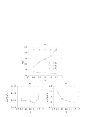
FIG. 1.: The dependence on $\eta$ of the mixing angles (a) and mass squared differences (b) and (c). For all data points except $\eta=1.0$, we have used $N=10$ instead of $N=20$.

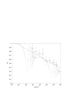
FIG. 2.: The “ratio of ratios” ${\cal R}$ as a function of $l\simeq 1.27L/E$. The data points are obtained from Fig. 4 in Ref. [32]. The dotted curve is a theoretical curve using the best point solution. The dashed and solid curves are obtained from the theoretical curve by using running average with different averaging lengths. The solid curve uses a larger averaging length than the dashed curve.