Imaging the Space-Time Evolution of High Energy Nucleus-Nucleus Collisions with Bremsstrahlung

Abstract

The bremsstrahlung produced when heavy nuclei collide is estimated for central collisions at the Relativistic Heavy Ion Collider. Bremsstrahlung photons with energies below 100 to 200 MeV are sufficient to discern the gross features of the space-time evolution of electric charge, if they can be separated from other sources of photons experimentally. This is illustrated explicitly by considering two very different models, one Bjorken-like, the other Landau-like, both of which are constructed to give the same final charge rapidity distribution.

             PACS numbers: 25.75.-q, 13.40.-f                                        preprint NUC-MINN-99/3-T

I Introduction

The Relativistic Heavy Ion Collider (RHIC) at Brookhaven National Laboratory (BNL) will have its first beam available for experiments by the end of 1999. A basic quantity of interest is the initial energy density of hot matter whose study is the ultimate physics goal. Hadronic measurements may not illuminate the state of the system at maximum density for two reasons: First, the system must expand and cool to a sufficiently low density before quarks and gluons can bind into independent color singlet hadrons. Second, even after hadronization or confinement phase transition the hadrons can scatter among themselves, changing their momentum distributions. For these reasons hard photons and lepton pairs have been considered better probes of the high temperature plasma of quarks and gluons since the production rate of such radiation increases dramatically with temperature. However, high transverse momentum photons and lepton pairs can also originate from the lower temperature hadronic phase due to hadron-hadron collisions and decays coupled with collective transverse expansion. (Focussing on high mass pairs negates this to some extent but eventually the Drell-Yan mechanism will overwhelm these at very high mass.) If it was only possible to see these nuclear collisions with the human eye! This is not possible, of course, leaving the next best option: Measurement of the electromagnetic bremsstrahlung produced by the massive deceleration of the nuclear electric charge.

The first theoretical study of nucleus-nucleus bremsstrahlung at relativistic energies, of order 1 GeV per nucleon, was carried out by one of the authors [1]. This was followed by Bjorken and McLerran who were interested in much higher beam energies [2], and then by Dumitru, McLerran and Stöcker [3]. Most recently Jeon, Kapusta, Chikanian and Sandweiss [4] studied bremsstrahlung photons with energies less than 5 MeV and a detector design to measure them at RHIC. Such an observation would allow for a determination of the final rapidity distribution of the net electric charge, which is one measure of transparency and stopping, obviously important for the initial energy density and the formation of quark-gluon plasma. It may be argued that a direct observation of all electrically charged hadrons would yield the same information, albeit at much higher cost. Nevertheless a cross check would be valuable.

In this paper, we wish to determine whether it is possible to discern the gross features of the space-time evolution of the electric charge using bremsstrahlung photons with energies up to 100 or 200 MeV in the lab frame of RHIC (which is also the center-of-mass frame for a collider). Generally a photon of energy 200 MeV would allow one to probe distances on the scale of 1 fm and times on the scale of 1 fm/c. At ultrarelativistic beam energies this is not quite true due to the extreme forward focussing of the bremsstrahlung. Nevertheless the answer to the question posed at the beginning of this paragraph is yes. In section 2, we work out the necessary formulas for bremsstrahlung. In section 3, we apply it to two extreme models: the first is Bjorken-like, which has considerable nuclear transparency, and the second is Landau-like, which has maximum nuclear stopping. Both models are tuned to produce a flat rapidity distribution for the net electric charge so that measurement of hadrons alone could not distinguish them. Section 4 contains concluding remarks.

II Calculation of Bremsstrahlung

Consider a central collision of two equal mass nuclei of charge $Z$ in their center of momentum frame. Denote the speed of each beam by $v_{0}$ and the corresponding rapidity by $y_{0}$, so that the rapidity gap between projectile and target nuclei is 2$y_{0}$. Velocity and rapidity are related by $v=\tanh y$. Before collision each nucleus may be viewed as a flattened pancake with negligible thickness since the photons we are considering cannot probe distances smaller than 1 fm. For example, with a RHIC beam energy of 100 GeV per nucleon the Lorentz $\gamma$ = 106 so that the diameter of a gold nucleus is contracted to 0.13 fm!

The formula for computing the classical bremsstrahlung from accelerated charges is well-known [5]. For charges $q_{i}$ with coordinates ${\bf r}_{i}(t)$, velocities ${\bf v}_{i}(t)$ and accelerations ${\bf a}_{i}(t)$ the intensity and number of photons emitted with frequency $\omega$ in the direction ${\bf n}$ are

$$\frac{d^{2}I}{d\omega d\Omega}=\omega\frac{d^{2}N}{d\omega d\Omega}=|{\bf A}|^{2}$$ (1)

where the amplitude is

$${\bf A}=\sum_{i}q_{i}\int_{-\infty}^{\infty}\frac{dt}{2\pi}\exp\left\{i\omega\left(t-{\bf n}\cdot{\bf r}_{i}(t)\right)\right\}\frac{{\bf n}\times\left[\left({\bf n}-{\bf v}_{i}(t)\right)\times{\bf a}_{i}(t)\right]}{\left(1-{\bf n}\cdot{\bf v}_{i}(t)\right)^{2}}\,.$$ (2)

The sum over charges may of course be replaced by an integral when the charge distribution is viewed as continuous.

A Soft bremsstrahlung

For low frequency photons, the nucleus-nucleus collision appears almost instantaneous. To the extent that the transverse rapidities of the outgoing charged particles are small compared to the beam rapidity one may then derive the formula [4]:

$$\frac{d^{2}I}{d\omega d\Omega}=\frac{\alpha}{4\pi^{2}}\sin^{2}\theta\left|\int d^{2}r_{\perp}\sigma(r_{\perp})e^{-i\omega{\bf n}\cdot{\bf r}_{\perp}}\left[\int dy\frac{v(y)\rho(r_{\perp},y)}{1-v(y)\cos\theta}-\frac{2v_{0}^{2}\cos\theta}{1-v_{0}^{2}\cos^{2}\theta}\right]\right|^{2}\,.$$ (3)

Here it is convenient to take ${\bf n}=\left(\sin\theta,0,\cos\theta\right)$. The function $\rho$ represents the charge rapidity distribution at a distance $r_{\perp}$ from the beam axis $z$ and is normalized as:

$$\int_{-\infty}^{\infty}dy\rho(r_{\perp},y)=2\,,$$ (4)

the 2 arising because the total charge is 2$Z$. We cannot go further without some knowledge of the distribution $\rho(r_{\perp},y)$.

It is advantageous to have a simple analytic model with a variable charge rapidity distribution. To this end, suppose that $\rho(r_{\perp},y)$ is independent of $r_{\perp}$. Then

$$\frac{d^{2}I}{d\omega d\Omega}=\frac{\alpha Z^{2}}{4\pi^{2}}\sin^{2}\theta\left|F(\omega\sin\theta)\right|^{2}\left|\left[\int dy\frac{v(y)\rho(y)}{1-v(y)\cos\theta}-\frac{2v_{0}^{2}\cos\theta}{1-v_{0}^{2}\cos^{2}\theta}\right]\right|^{2}\,,$$ (5)

where $F$ is a transverse nuclear form factor:

$$F=\frac{1}{Z}\int d^{2}r_{\perp}\,\sigma\left(r_{\perp}\right)e^{-i\omega{\bf n}\cdot{\bf r}_{\perp}}\,,$$ (6)

where $\sigma$ is the charge per unit area of the nucleus. A solid sphere approximation should be adequate for large nuclei, in which case

$$F(q)=\frac{3}{q^{2}}\left(\frac{\sin q}{q}-\cos q\right)\,,$$ (7)

where $q=\omega R\sin\theta$ and $R$ is the nuclear radius. For small angles and low frequencies the nuclear form factor is practically equal to one.

The integral over rapidity can easily be performed for a flat rapidity distribution: $\rho(y)=1/y_{0}$ for $-y_{0}<y<y_{0}$. Then the photon distribution is:

$$\frac{d^{2}I}{d\omega d\Omega} = \frac{\alpha Z^{2}}{4\pi^{2}}\sin^{2}\theta\left|F(\omega R\sin\theta)\right|^{2}$$ (8)

$$\times \left[\frac{2\cos\theta}{\sin^{2}\theta}-\frac{1}{y_{0}\sin^{2}\theta}\ln\left(\frac{1+v_{0}\cos\theta}{1-v_{0}\cos\theta}\right)-\frac{2v_{0}^{2}\cos\theta}{1-v_{0}^{2}\cos^{2}\theta}\right]^{2}\,.$$ (9)

Because $v_{0}$ is close to 1 the distribution deviates strongly from the quadrupole form, peaking near small but nonzero $\theta$. At RHIC the peak occurs at $\theta\sim 1^{\circ}$. The distribution is plotted in Fig. 1 for central gold collisions at RHIC with $\omega<<1/R=30$ MeV.

FIG. 1.: The intensity as a function of angle for very soft photons which results from a flat charge rapidity distribution. The intensity is independent of frequency for $\omega\ll 1/R$.

B Hard bremsstrahlung

All the results above were already reported in [4] and are applicable for very soft photons. Here we will consider photons with energies up to 100 to 200 MeV with the expectation that they will reveal the spatial and temporal development of the nuclear collision. We will consider only central collisions which can be triggered on experimentally with hadronic detectors, such as a calorimeter.

For this purpose one can certainly invoke specific space-time models of nuclear collisions at RHIC. In this paper we will consider simple parameterizations of such collisions which represent extreme limits of such models. The general formulas will be worked out here, in this section, and then applied to these models in the next section.

We will represent a large nucleus, such as gold, by a uniform spherical distribution of nucleons with proper density $n_{0}=0.155$ nucleons/fm³. An infinitesimal unit of charge will have a coordinate specified by $r_{\perp}$ and by the distance $l$ parallel to the $z$-axis as measured from the backside of the nucleus. For given $r_{\perp}$ the allowed value of $l$ ranges from 0 to $l_{max}(r_{\perp})=2\sqrt{R^{2}-r_{\perp}^{2}}$. Summation over all charges $i$ in eq. (2) is then replaced by an integral over ${\bf r}_{\perp}$ and $l$. See Fig. 2.

Each charge element undergoes some deceleration to a final rapidity y. This deceleration will take a finite time and can vary from one element to another. In this paper we will fix the final observed charge rapidity distribution and vary the space-time evolution to see whether hard bremsstrahlung can provide information not obtainable by measuring hadrons only. For definiteness we shall fix the final charge rapidity distribution to be flat. In individual nucleon–nucleon collisions it is known to be approximately proportional to $\cosh y$ in the center-of-momentum frame [6]. In order to obtain a flat rapidity distribution in a central nucleus-nucleus collision different charge elements must have a rapidity that depends on $r_{\perp}$. The assumed relationship among these variables is

$$l=f(r_{\perp})y+g(r_{\perp})\sinh y$$ (10)

where $f$ and $g$ are functions yet to be specified. This means that the last charge element in line will eventually come to rest in the center-of-momentum frame.

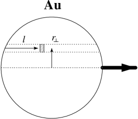
FIG. 2.: The charge element coordinate labels in the rest frame of the nucleus.

The charge per unit area per unit rapidity is:

$$\frac{d^{3}Q}{d^{2}r_{\perp}dy}=n_{0}\frac{Z{\rm e}}{A}\frac{dl(r_{\perp},y)}{dy}=n_{0}\frac{Z{\rm e}}{A}\left[f(r_{\perp})+g(r_{\perp})\cosh y\right]\,.$$ (11)

To have a net flat rapidity distribution requires that

$$\int_{0}^{R}dr_{\perp}r_{\perp}g(r_{\perp})=0\,.$$ (12)

As $r_{\perp}\rightarrow R$ the distribution should have a minimum at $y=0$, in accord with proton-proton scattering, whereas when $r_{\perp}\rightarrow 0$ the distribution must have a maximum at $y=0$ to produce a distribution that is flat overall. This is physically sensible because there ought to be significantly more deceleration in the central core of the nucleus than at its outer periphery. A linear extrapolation of nucleon-nucleon scattering to central collisions of gold nuclei at RHIC [4, 6] produces just such a behavior with a net distribution that is approximately flat in rapidity. We choose the parameterization $g(r_{\perp})=g_{1}l_{max}(r_{\perp})-g_{2}l^{2}_{max}(r_{\perp})$ where $g_{1}$ and $g_{2}$ are positive constants. The requirement of a net rapidity distribution which is flat results in $g_{2}=2g_{1}/3R$. The physically sensible requirement that the leading charge elements emerge from the collision with the original beam rapidity determines the function $f(r_{\perp})$ via $l_{max}(r_{\perp})=f(r_{\perp})y_{0}+g(r_{\perp})\sinh y_{0}$. Finally, the requirement that the charge rapidity distribution be non–negative for all allowable $y$ leads to the condition $g_{1}\leq 3/(y_{0}\cosh y_{0}-\sinh y_{0})$. For definiteness we choose the upper limit $g_{1}=3/(y_{0}\cosh y_{0}-\sinh y_{0})$ since this value brings the rapidity distribution as close to $\cosh y$ as $r_{\perp}\rightarrow R$ as possible, consistent with free space nucleon-nucleon scattering. The resulting $d^{3}Q/d^{2}r_{\perp}dy$ is plotted in Fig. 3, and is very similar to what is obtained in LEXUS (see Fig. 1 of [4]).

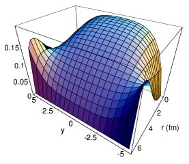
FIG. 3.: The charge rapidity distribution, $d^{3}Q/d^{2}r_{\perp}dy$, as it depends on the transverse coordinate $r_{\perp}$.

For a central collision of equal mass nuclei at RHIC the primary accelerations occur along the direction of the beam axis. By azimuthal symmetry the transverse accelerations will, in addition, tend to cancel in the expression for the amplitude. The contribution to the amplitude from the projectile will then be:

$$A_{+} = \sin\theta\frac{Z{\rm e}}{A}n_{0}\int_{0}^{R}dr_{\perp}r_{\perp}J_{0}(r_{\perp}\omega\sin\theta)\int_{0}^{l_{max}(r_{\perp})}dl$$ (13)

$$\times \int_{-\infty}^{\infty}dt\exp\{i\omega\left(t-z(l,t)\cos\theta\right)\}\frac{a(l,t)}{(1-v(l,t)\cos\theta)^{2}}\,.$$ (14)

The expression for the contribution from the target nucleus $A_{-}$ will be the same except for the reversal of sign of the position, velocity, and acceleration. Since there is a one-to-one relation between the longitudinal label $l$ and the rapidity $y$ this amplitude may be written as an integral over $y$ instead of over $l$ as:

$$A_{+} = \sin\theta\frac{Z{\rm e}}{A}n_{0}\int_{0}^{R}dr_{\perp}r_{\perp}J_{0}(r_{\perp}\omega\sin\theta)\int_{0}^{y_{0}}dy\frac{dl(y,r_{\perp})}{dy}$$ (15)

$$\times \int_{-\infty}^{\infty}dt\exp\{i\omega\left(t-z(y,t)\cos\theta\right)\}\frac{a(y,t)}{(1-v(y,t)\cos\theta)^{2}}\,.$$ (16)

For a specified model of the deceleration this three-dimensional integral must be evaluated numerically.

III Two Extreme Models

In this section we will describe two extreme models for the space-time evolution of a central nucleus-nucleus collision at RHIC. The real world will undoubtedly be different than either of these. However, our point is that hard bremsstrahlung may be used to discern the gross features of the evolving charged matter, something that hadron detection alone cannot do because the final charge rapidity distribution in these two models is the same (by construction).

A A Bjorken-like model

This model assumes that the nucleons undergo a constant deceleration upon nuclear overlap. It essentially assumes transparency [7] of electric charge although the final charge rapidity distribution is assumed to be flat. Because the nuclei are so highly Lorentz contracted initially it is an excellent approximation to assume that all charge elements are located at $z=0$ at the moment $t=0$ of complete nuclear overlap. A photon with energy less than 200 MeV would never be able to distinguish this from a Lorentz contracted pancake of thickness 0.13 fm! For a projectile charge element with nuclear coordinates $l,r_{\perp}$ the position as a function of time is:

$${z(l,r_{\perp},t)\,=\,\left\{\begin{array}[]{ll}v_{0}t&t<0\\ v_{0}t+a(l,r_{\perp})t^{2}/2&0<t<t_{f}\\ z(l,r_{\perp},t_{f})+v_{f}(t-t_{f})&t_{f}<t\,.\end{array}\right.}$$ (20)

The deceleration is

$$a(l,r_{\perp})=\frac{v_{f}-v_{0}}{t_{f}}=\frac{\tanh y-\tanh y_{0}}{t_{f}}\,.$$ (21)

Remember that $l$ and $v_{f}=\tanh y$ are related by eq. (9). The trajectory of a target charge element is obtained symmetrically. Note that the charges continue to decelerate even after the nuclei have passed through each other. This may be thought of as strings connecting projectile and target charges causing them to decelerate at a distance, or by the finite time necessary for particle production.

The deceleration time $t_{f}$ is allowed to depend on the length of the tube as follows:

$$t_{f}(r_{\perp})=t_{0}+l_{max}(r_{\perp})/c_{0}$$ (22)

where $t_{0}$ and $c_{0}$ are constants. Several choices of these parameters will be considered.

B A Landau-like model

This model assumes that the nuclei stop each other within a distance of one Lorentz contracted nuclear diameter, then accelerate longitudinally due to the high pressure [8]. The deceleration occurs over such a short time interval that photons of 200 MeV or less cannot resolve it. Thereafter our variation of Landau’s model assumes that the charge elements accelerate uniformly to their final velocities. The trajectories are parameterized as:

$$a(l,r_{\perp})=-v_{0}\delta(t)+\frac{v_{f}}{t_{f}}\theta(t)\theta(t_{f}-t)\,.$$ (23)

The relationship among $l$, $v_{f}$ and $y$ is as above. In a hydrodynamical approach the final time $t_{f}$ is expected to be independent of $r_{\perp}$ but it can be left as a parameter, just as in the Bjorken-like model.

C Comparison of models

Before comparing the bremsstrahlung produced in these two models let us compare the space-time evolutions. In Fig. 4 we plot cells bounded by lines of constant $l$ and $r_{\perp}$ in the $x-z$ plane as a function of time. Each cell contains the same amount of charge. The left panel shows the Bjorken-like model and the right panel shows the Landau-like model. Both models have $t_{f}=1$ fm/c; that is, the acceleration time is independent of $r_{\perp}$. There are several noteworthy features: The Bjorken-like model always has a gap in the beam direction because it takes a finite time for the charges to decelerate. The charges that finally come to rest in this frame of reference require 1 fm/c to decelerate from $v=\pm v_{0}$ to $v=0$ and by then they have traveled 0.5 fm. In contrast, the charges in the Landau-like model stop instantaneously and then accelerate to their final velocities. Therefore there is no gap in the beam direction. Note that the shaded regions indicate where the net charge is nonzero. The gap in the central region in the Bjorken-like model does not signify empty space but rather a region where there is zero net charge; it may be occupied by quark-gluon plasma or hadronic matter or strings or something else.

                 

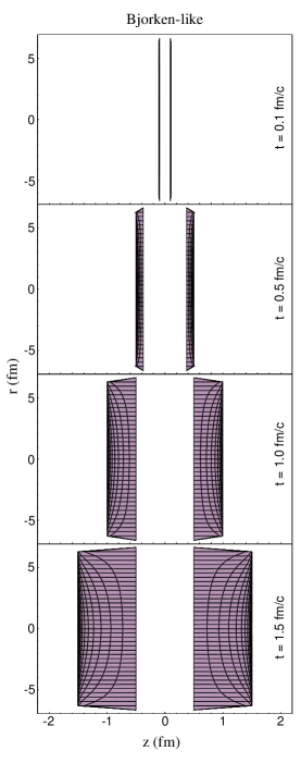
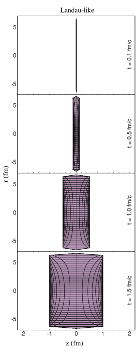
FIG. 4.: Space-time evolution in a Bjorken-like model compared to that of a Landau-like model both with $t_{f}=1$ fm/c. The curves indicate contours of constant $l$ and $r_{\perp}$ and so each cell, as delineated this way, contains the same amount of electric charge.

In Fig. 5 we show the space-time evolution for $t_{0}=0.5$ fm/c and $c_{0}=1$ in the Bjorken-like model and for $t_{0}=10$ fm/c and $c_{0}=\infty$ in the Landau-like model. We chose the acceleration time in the Landau-like model to be independent of $r_{\perp}$ because this seems more relevant for a hydrodynamical model. In the Bjorken-like model we chose the minimum time $t_{0}=0.5$ fm/c because, even in free space, nucleon-nucleon collisions must occur over some finite time interval. The value of 0.5 fm/c is suggested by the analysis of Gale, Jeon and Kapusta [9] of Drell-Yan and $J/\psi$ production in very high energy proton-nucleus collisions. The central cores of the gold nuclei then require 13.9 fm/c to decelerate to their final velocities. Hence the average deceleration time ought to be comparable to the 10 fm/c chosen for the Landau-like model. Apart from the quantitative difference in the space-time evolution, the gap in the Bjorken-like model is now more like an ellipse than a slab.

                 

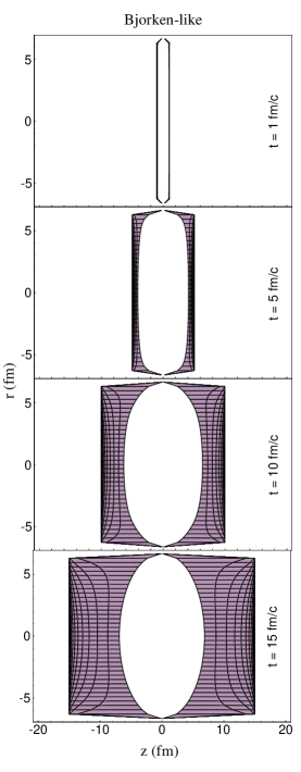
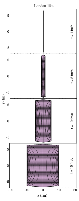
FIG. 5.: Same as Fig. 4 except that the Bjorken-like model has a $t_{f}$ varying from 0.5 fm/c at $r_{\perp}=R$ to 13.9 fm/c at $r_{\perp}=0$, and the Landau-like model has fixed $t_{f}=10$ fm/c.

The intensity distribution in the Bjorken-like model is plotted in Fig. 6 for the angles 1^o, 5^o, 10^o and 20^o. Three values of $c_{0}$ have been chosen for display: 0.5, 1 and $\infty$. The value of $t_{0}$ has been fixed at 0.5 fm/c in all cases, although the results are practically the same with any $t_{0}<1$ fm/c. The three values of $c_{0}$ correspond to final times for the central cores of 27.3, 13.9 and 0.5 fm/c, respectively. (Be careful to note the false zeroes in three of the four panels.) The dependence on $c_{0}$ is very weak considering the wide range of resulting $t_{f}$. This may be understood as a relativistic effect. Because of the relation $v=\tanh y$, most of the outgoing charges still move with a speed nearly equal to that of light. Therefore the phase in eqs. (12-13) is approximately $i\omega t(1-\cos\theta)$, and for it to become comparable to 1 requires an $\omega$ much bigger than naively expected. The separation of the curves increases with $\theta$ following this phase factor. The primary falloff of the intensity with increasing photon energy is caused by the transverse form factor described by eq. (7). The falloff increases with angle because the argument of the form factor is $q=\omega R\sin\theta$.

The intensity distribution in the Landau-like model is plotted in Fig. 7 for the same set of angles. Four illustrative values of $t_{f}$ have been chosen: 1, 2, 10 and 20 fm/c. In this model there is a striking dependence on $t_{f}$. The oscillatory behavior for large $t_{f}$ is due to the interference between the initial instantaneous stopping with the subsequent acceleration to the final velocities. At 10^o and with $t_{f}=20$ fm/c, for example, the enhancement due to constructive interference is an order of magnitude at $\omega=60$ MeV as compared to the soft photon limit.

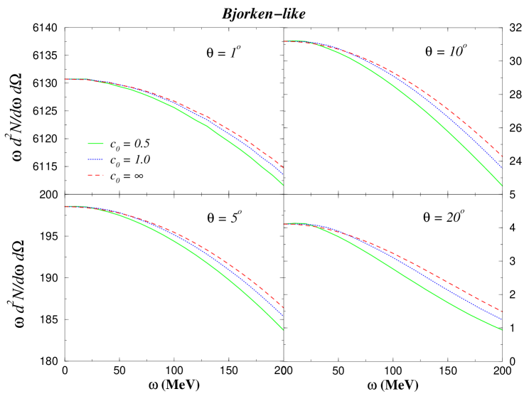
FIG. 6.: The intensity distribution in the Bjorken-like model as a function of photon energy for various angles. The three curves correspond to different acceleration times.

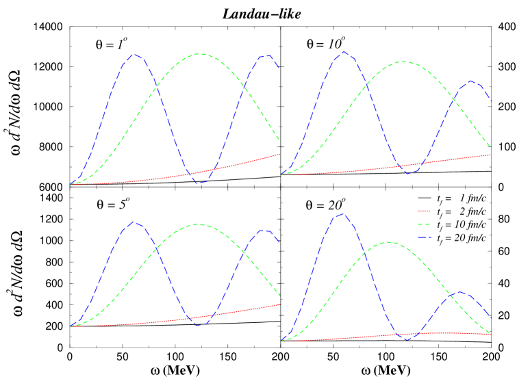
FIG. 7.: The intensity distribution in the Landau-like model as a function of photon energy for various angles. The four curves correspond to different acceleration times.

The oscillatory behavior which arises in the Landau-like model but not in the Bjorken-like model is easy to understand in a simplified version of these models. Let us shrink each nucleus to a point charge. In the Bjorken-like version, assume that the charges decelerate from $\pm v_{0}$ to $\pm v_{f}$ instantaneously. The intensity distribution is:

$$\frac{d^{2}I}{d\omega d\Omega}=\frac{Z^{2}\alpha}{\pi^{2}}\sin^{2}\theta\cos^{2}\theta\frac{(v_{0}^{2}-v_{f}^{2})^{2}}{(1-v_{0}^{2}\cos^{2}\theta)^{2}(1-v_{f}^{2}\cos^{2}\theta)^{2}}\,,$$ (24)

which has no frequency dependence. In the Landau-like version assume that the charges stop instantaneously, remain at rest for a time $\tau$, then instantly accelerate to final velocities $\pm v_{f}$. This intensity distribution is:

$$\frac{d^{2}I}{d\omega d\Omega} = \frac{Z^{2}\alpha}{\pi^{2}}\sin^{2}\theta\cos^{2}\theta\left\{\frac{[v_{0}^{2}-v_{f}^{2}\cos\omega\tau-v_{0}^{2}v_{f}^{2}(1-\cos\omega\tau)\cos^{2}\theta]^{2}}{(1-v_{0}^{2}\cos^{2}\theta)^{2}(1-v_{f}^{2}\cos^{2}\theta)^{2}}\right.$$ (25)

$$+ \left.\frac{v_{f}^{4}\sin^{2}\omega\tau}{(1-v_{f}^{2}\cos^{2}\theta)^{2}}\right\}\,.$$ (26)

The period of oscillation is just the time delay between stopping and sudden acceleration. This is essentially what happens in the Landau-like model, modified by the smearing which follows from a continuous acceleration rather than a time delayed one, and by the relativistic effect in the phase factor as mentioned before.

IV Conclusion

In this paper we have studied two very different and extreme models of the space-time evolution of the charges in central nucleus-nucleus collisions at a RHIC energy of 100 GeV per nucleon in the center of mass frame. The models were constructed to yield the same final rapidity distribution of the net outgoing electric charge. This means that measurement of hadron spectra alone cannot discern them. Very low energy bremsstrahlung cannot discern them either because it depends only on the difference between the incoming and outgoing currents, which are identical. Bremsstrahlung photons of higher energy can distinguish these extreme models. For the Landau-like model photons of energy 100 MeV or so is quite sufficient to infer the time scale for expansion. Bremsstrahlung photons with energy up to 200 MeV may be able to infer the deceleration time in Bjorken-like models but one needs to look at angles much greater than where the peak of the spectrum occurs, which is 1 degree. Whether it is really possible to design a detector that can separate other sources of photons of this energy is an open question, but at least we have shown that the physics to be learned is interesting, perhaps justifying an experimental effort [10].

REFERENCES

- [1] J. Kapusta, Phys. Rev. C 15, 1580 (1977).
- [2] J. D. Bjorken and L. McLerran, Phys. Rev. D 31, 63 (1985).
- [3] A. Dumitru, L. McLerran, H. Stocker and W. Greiner, Phys. Lett. B 318, 583 (1993).
- [4] S. Jeon, J. Kapusta, A. Chikanian and J. Sandweiss, Phys. Rev. C 58, 1666 (1998).
- [5] J. D. Jackson, Classical Electrodynamics, 2nd ed. (Wiley, N.Y. 1975). Note that our paper follows this text in defining .
- [6] S. Jeon and J. Kapusta, Phys. Rev. C 56, 468 (1997).
- [7] J. D. Bjorken, Phys. Rev. D 27, 140 (1983).
- [8] L. D. Landau, Izv. Akad. Nauk SSSR (Physics Series) 17, 51 (1953); S. Z. Belenkij and L. D. Landau, Uspekhi Fiz. Nauk, 56, 309 (1955) and Nuovo Cimento Suppl. 3, 15 (1956).
- [9] C. Gale, S. Jeon and J. Kapusta, Phys. Rev. Lett. 82, 1626 (1999); ibid. preprint nucl-th/9812056, submitted to Phys. Lett. B.
- [10] Jack Sandweiss, private communication.