Abstract

The production of a Higgs boson in association with a $W$-boson is the most likely process for the discovery of a light Higgs at the Fermilab Tevatron. Since it decays primarily to $b$-quark pairs, the principal background for this associated Higgs production process is $Wb\bar{b}$, where the $b\bar{b}$ pair comes from the splitting of an off mass shell gluon. In this paper we investigate whether the spin angular correlations of the final state particles can be used to separate the Higgs signal from the $Wb\bar{b}$ background. We develop a general numerical technique which allows one to find a spin basis optimized according to a given criterion, and also give a new algorithm for reconstructing the $W$ longitudinal momentum which is suitable for the $WH$ and $Wb\bar{b}$ processes.

1 Introduction

At present, the existence of a neutral Higgs boson is certainly the largest unresolved problem in the standard model (SM). Its mass is a priori unknown, but direct searches and precision electroweak measurements constrain it to be $90<M_{H}<280{\;\rm GeV}$ at 95% confidence level [1]. At the Tevatron collider there is a possibility to search for the SM Higgs using the decay mode $H\rightarrow b\bar{b}$ [2], and the most promising process is the associated Higgs production

$$p\bar{p}\rightarrow W(\rightarrow e\nu)H(\rightarrow b\bar{b})\ .$$ (1)

The Fermilab search is extremely important, especially because the mass range which can be covered at the Tevatron ($100<M_{H}<130{\;\rm GeV}$) is also one of the most challenging regions for the LHC to look for the SM Higgs [3]. With sufficiently large data sample the Higgs signal could be extracted from the background by analyzing the $b\bar{b}$ mass distribution. However, given the fact that there are several large backgrounds to process (1), any technique which can provide additional handles on distinguishing the signal from the background would be useful.

In this paper we investigate the possibility of using the spin angular correlations for separating the associated Higgs production from its principal background at the Tevatron, the $Wb\bar{b}$ process

$$p\bar{p}\rightarrow W(\rightarrow e\nu)g^{*}(\rightarrow b\bar{b})\ .$$ (2)

In the case of $e^{+}e^{-}\rightarrow ZH/ZZ$ in [4] it was shown that spin angular correlations can provide useful information if good spin bases are chosen. Since the $q\bar{q}\rightarrow WH/Wb\bar{b}$ processes have the same spin structure, it is natural for one to ask a question whether a similar analysis would be useful for distinguishing (1) and (2) at the Tevatron. However, due to the hadronic collider environment, and also to the complexity of the $Wb\bar{b}$ amplitudes, it is obvious that in this case a numerical approach for finding the best spin basis is more appropriate than the approach used in [4]. For that reason we develop here a new method which allows one to find a spin basis optimized according to a given criterion. This technique is completely general in the sense that it can be used for optimizing spin basis regardless of which or how many processes are being considered. We apply our method to $WH$ and $Wb\bar{b}$ processes, and suggest several possible strategies which could add new information in an experimental analysis. We also discuss one of the major uncertainties related to our analysis, and that is the $W$ momentum reconstruction. Our results indicate that the method which has been used in the literature can distort angular distributions considerably, and is therefore inadequate for our purposes. Because of that we propose a new $W$ reconstruction algorithm whose effects on angular distributions are significantly less destructive.

The remainder of the paper is organized as follows: in Section 2 we give all relevant definitions, describe numerical method and suggest possible strategies for finding the optimal spin basis. In Section 3 we present our results for angular distributions, and show the effects which $W$ reconstruction algorithm has on those. Conclusions are contained in Section 4.

2 Angular correlations

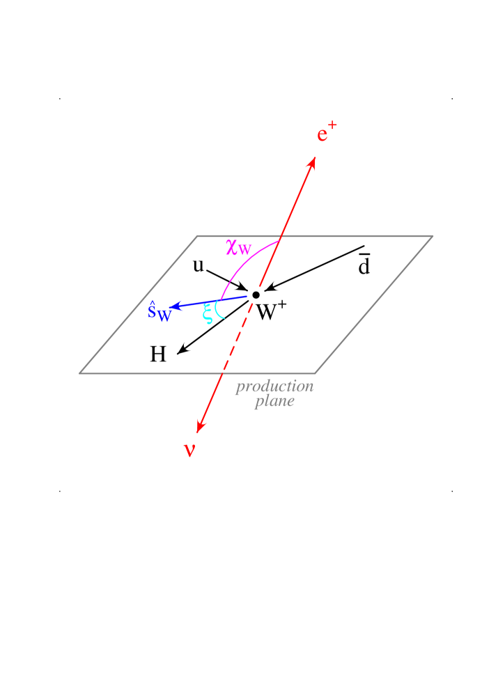
Figure 2: Definitions for angles $\xi$ and $\chi_{W}$ in the $W$ rest frame.

In order to apply the generalized spin-basis analysis [5] to processes (1) and (2) we first define the zero momentum frame (ZMF) production angle $\theta^{*}$ ($0\leq\theta^{*}<\pi$) as the angle between the incoming up-quark and the $W$-boson produced in the $q\bar{q}^{\prime}\rightarrow WX$ process (see Figure 1), where $X$ is either $H$ or $g^{*}$. The spin states for $W$ are defined in its rest frame, where we decompose its spin along the vector $\hat{s}_{W}$, which makes an angle $\xi$ with the $X$ particle momentum in the clockwise direction. The $X$ particle’s spin can be decomposed in a similar way. Relationship between $\xi$ and $\theta^{*}$ determines specific spin basis in which one can calculate angular correlations among the $WH$ and $Wg^{*}$ decay products in (1) and (2). These correlations involve distributions of the angle $\chi_{W}$ ($\chi_{b\bar{b}}$) that the charged lepton ($b$-quark) makes with the spin vector of the $W$-boson ($b\bar{b}$ system). Figure 2 illustrates the definitions for angles $\xi$ and $\chi_{W}$.

In the case of $e^{+}e^{-}\rightarrow ZH/ZZ\rightarrow l\bar{l}\;jets$ the procedure for finding the optimal spin basis was based on separating the polarized amplitudes for $e^{+}e^{-}\rightarrow ZH/ZZ$ [4]. In particular, it was shown that very good separation between the $ZH$ and $ZZ$ events can be obtained in the transverse basis, in which the longitudinal component of the $ZH$ matrix element is zero by construction.

Since the amplitude for the process $q\bar{q}^{\prime}\rightarrow WH$ has the same spin structure as the one for $e^{+}e^{-}\rightarrow ZH$, the transverse basis is also a good starting point for examining the $\cos{\chi}$ distributions in the $WH$ and $Wb\bar{b}$ processes. It is defined by

$$\tan{\xi}={\tan{\theta^{*}}\over\sqrt{1-\beta^{2}_{W}}}\ ,$$ (3)

where $\beta_{W}$ is the ZMF speed of the $W$-boson. Nevertheless, due to the complex nature of the $q\bar{q}^{\prime}\rightarrow Wg^{*}$ amplitudes, and also to the fact that in $p\bar{p}$ collisions the center-of-mass energy $\sqrt{\hat{s}}$ is not fixed, the approach of Ref. [4] for finding the optimal spin basis is not practical for our purposes here. Because of that, instead of trying to separate polarized cross sections for $q\bar{q}^{\prime}\rightarrow WH/Wg^{*}$, we attempt to find the best basis for processes (1) and (2) by distinguishing the $\cos{\chi}$ distributions directly, using a suitable multidimensional maximization procedure.

The basic idea of our method is to divide $\cos{\theta^{*}}-\cos{\xi}$ plane into $n\times m$ regions, and to associate with each of those a histogram containing distribution in $\cos{\chi}$. A specific spin basis is defined by choosing one of the $\cos{\xi}$ bins for all of $n$ $\cos{\theta^{*}}$ bins, while the total $\cos{\chi}$ distribution is obtained by summing contributions over the entire $\cos{\theta^{*}}$ range. In other words, if $\cos{\xi_{i}}$ describes the spin vector of $W$ (or $b\bar{b}$ system) in the $i$-th $\cos{\theta^{*}}$ bin, and $\sigma_{i}$ is the corresponding contribution to the cross section, we have

$$\frac{d\sigma}{d\cos{\chi}}=\sum_{i=1}^{n}\frac{d\sigma_{i}(\cos{\xi_{i}})}{d\cos{\chi}}\ .$$ (4)

In this way, by changing the $n$ $\cos{\xi_{i}}$ variables using multidimensional maximization algorithm, one can easily vary the definition of the spin basis until the optimal separation of the $WH$ and $Wb\bar{b}$ events is achieved.

Results of this procedure will clearly depend on which criterion is used for determining the best possible separation of the signal and the background. We investigate here two possible criteria. The first one is based on distinguishing between the shapes of the $\cos{\chi}$ distributions for the two processes, and the function which we decided to maximize is given by

$$\left|\frac{1}{\sigma_{WH}}\int d\cos{\chi}\frac{d\sigma_{WH}}{d\cos{\chi}}\cos{\chi}\right|-\left|\frac{1}{\sigma_{Wb\bar{b}}}\int d\cos{\chi}\frac{d\sigma_{Wb\bar{b}}}{d\cos{\chi}}\cos{\chi}\right|\ .$$ (5)

With this criterion the resulting spin basis tends to give $\cos{\chi}$ distributions which are asymmetric for the $WH$ signal events and symmetric for the $Wb\bar{b}$ background events.

The second criterion which we examine is based on maximizing significance $S/\sqrt{B}$, where $S$ and $B$ correspond to the number of events for the signal and background, respectively:

$$S \propto \int_{\cos{\chi_{min}}}^{\cos{\chi_{max}}}d\cos{\chi}\frac{d\sigma_{WH}}{d\cos{\chi}}\ ,$$ (6)

$$B \propto \int_{\cos{\chi_{min}}}^{\cos{\chi_{max}}}d\cos{\chi}\frac{d\sigma_{Wb\bar{b}}}{d\cos{\chi}}\ .$$ (7)

Once a particular spin basis is chosen and the $\cos{\chi}$ distribution for both processes is calculated using (4), we choose angles ${\chi_{min}}$ and ${\chi_{\max}}$ in such a way to maximize the ratio $S/\sqrt{B}$. Note that in the above coefficients of proportionality include the NLO $K$-factors, our assumptions on the integrated luminosity and double $b$-tagging efficiency, etc.

The main advantage of the method described above is that it offers a systematic approach for investigating the possibility of using the spin angular correlations to distinguish signal events from the background, regardless of which or how many processes are being considered. For example, even though we are concerned here only with the leading order $Wb\bar{b}$ process as the most important background for the associated Higgs production at the Tevatron, it would be straightforward to include other backgrounds or the next-to-leading order effects as well. Note however that calculation of angular correlations between the spin vector of an intermediate gauge boson and momenta of its decay products requires complete reconstruction of an event. That is a major difficulty in the case of the $WH/Wb\bar{b}$ production where longitudinal component of neutrino is unknown. This issue will be discussed in more details in the following section.

3 Numerical results

Since the procedure outlined above requires large statistics in order to make errors in $d\sigma/d\cos{\chi}$ distributions as small as possible, for the results presented in this paper we generated about $10^{8}$ events (for each process), using the VEGAS algorithm [7]. Calculations were done with $n=10$ bins along the $\cos{\theta^{*}}$ axis, and $m=1000$ bins along the $\cos{\xi}$ axis, while the search for the optimal basis was performed using the downhill simplex method [10, 11].

Even though the analysis described in the previous section can be performed for both $W$ and $b\bar{b}$ sides of an event, we focus here only on the $\cos{\chi_{W}}$ distributions. The reason is that the correlations on the $W$ side of an event are much stronger and provide us with more distinguishing power for separating the $WH$ and $Wb\bar{b}$ processes.

All results shown in this paper are obtained for the $W^{+}$ production in $p\bar{p}$ collisions at $\sqrt{S}=2{\;\rm TeV}$, with the MRSR1 parton distribution functions ($\alpha_{S}(M_{Z})=0.113$) [12]. In order to improve our lowest order cross sections, instead of natural scales ($\mu\approx M_{H}$) we used somewhat lower scale of $\mu=50{\;\rm GeV}$ [13]. At this scale the NLO $K$-factors are about 1.1 for both $WH$ and $Wb\bar{b}$ processes. The Higgs mass was set to $M_{H}=120{\;\rm GeV}$ and the corresponding $b\bar{b}$ mass range to $102<M_{b\bar{b}}<141{\;\rm GeV}$. In addition, we applied the following set of isolation cuts and cuts on rapidity and transverse momentum:

$$\begin{array}[]{rcl}R_{b\bar{b}},R_{eb},R_{e\bar{b}}&>&0.7\ ,\\ |y_{b}|,|y_{\bar{b}}|&<&2\ ,\\ |y_{e}|&<&2.5\ ,\\ |p^{T}_{b}|,|p^{T}_{\bar{b}}|&>&15{\;\rm GeV}\ ,\\ |p^{T}_{e}|,|p^{T}_{\nu}|&>&20{\;\rm GeV}\ .\end{array}$$ (8)

Note the $|p^{T}_{\nu}|$ cut is the missing $E_{T}$ cut and that the above cuts do not include a cut on $\cos{\theta^{*}}$ [14]. Our results indicate that imposing the $\cos{\theta^{*}}$ cut actually worsens our ability to separate the two processes based on the shape of their $\cos{\chi_{W}}$ distributions, and therefore we did not include it in the simulations based on maximization of Eq. (5). On the other hand, it is well known that this cut can improve the $S/\sqrt{B}$ ratio by about 10% [14]. Because of that, we take it into account for simulations based on the significance criterion.

We first discuss our results obtained with the shape criterion. In this case we found that the optimal basis can be well approximated by the polynomial of the form

$$\cos{\xi}=\sum_{i=1}^{k}a_{i}(\cos{\theta^{*}})^{2i-1}\ .$$ (9)

In particular, in Figure 3 we compare the exact result obtained by maximization procedure to polynomial with $k=3$ and coefficients

$$a_{1} = 0.2354\ ,$$

$$a_{2} = 0.1808\ ,$$ (10)

$$a_{3} = -1.442\ .$$

There we also show the transverse basis with specific choice of $\beta_{W}=0.67$, which is close to the averages of the $\beta_{W}$ distributions for both $WH$ and $Wb\bar{b}$ processes (0.68 and 0.66, respectively). The actual normalized $\cos{\chi_{W}}$ distributions corresponding to the polynomial approximation of the optimal basis and for the transverse basis are given in Figure 4. As expected, in the optimal basis the $Wb\bar{b}$ distribution is nearly symmetric. Figures 5 and 6 illustrate what one might expect in terms of the number of events per bin in those two bases. These results were obtained by multiplying our $W^{+}$ cross sections by four to take into account contributions from the $W^{-}$ production and the contribution from the $W^{\pm}$ decays into muons, by taking into account the NLO $K$-factor of 1.1 for both $WH$ and $Wb\bar{b}$ processes, and also by assuming the double $b$-tagging efficiency of $\epsilon_{b}^{2}=0.45$ and integrated luminosity of $10{\rm\;fb}^{-1}$. We would like to point out here that the shape of the $Wb\bar{b}$ $\cos{\chi_{W}}$ distribution is significantly different in the two bases being discussed. On the other hand, this is not the case for the $WH$ process. Clearly, the difference in the shape of the $\cos{\chi_{W}}$ distributions under the change of spin basis may provide an additional handle for separating the two processes.

Another interesting possibility of using angular correlations for distinguishing between the signal and the background is illustrated in Figures 7 through 9. Instead of looking at $d\sigma/d\cos{\chi_{W}}$ directly, we investigate the $M_{b\bar{b}}$ distributions of the quantity $\sigma\cos{\chi_{W}}$. Those distributions vanish in the spin basis in which $d\sigma/d\cos{\chi_{W}}$ is perfectly symmetric, because in evaluating $d(\sigma\cos{\chi_{W}})/dM_{b\bar{b}}$ one effectively integrates over $\cos{\chi_{W}}$. This is precisely the reason why our optimal basis reduces the background in $\sigma\cos{\chi_{W}}$ much more efficiently than the transverse basis, as can be seen by comparing Figures 8 and 9. However, at this point one should also observe that the main disadvantage of analyzing quantities such as $\sigma\cos{\chi_{W}}$ is the inclusion of the statistical errors of the entire $\cos{\chi_{W}}$ distribution, which may limit its potential usefulness in an experimental analysis with small statistics.

In our simulations based on maximizing significance the number of events for both signal and background was obtained by summing all decay channels, and under the same assumptions as before ($K$-factors of 1.1, $\epsilon_{b}^{2}=0.45$, and $\int{\cal L}\;dt=10{\rm\;fb}^{-1}$). As mentioned earlier, besides cuts given in (8), here we also take into account a cut on $\cos{\theta^{*}}$ [14],

$$|\cos{\theta^{*}}|\leq\cos{\theta^{*}_{max}}\ ,$$ (11)

which can increase the ratio $S/\sqrt{B}$ by about 10% (see Table 1). Using the method described in Section 2, and for any given value of $\cos{\theta^{*}_{max}}$, we were able to find a spin basis (and a set of cuts on $\cos{\chi}$) in which one could further improve this ratio by additional 2-3%.

Our results with $\cos{\theta_{max}}=0.8$ are shown in Figures 10 through 13. Figure 10 shows the optimal basis definition. In this case we found that it can be approximated by

$$\cos{\xi}=-0.857\;{\rm sign}(\cos{\theta^{*}})+0.391\cos{\theta^{*}}\ .$$ (12)

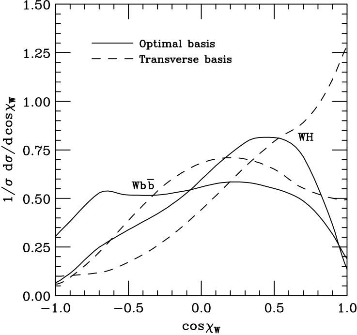
Figure 11: Normalized $\cos{\chi_{W}}$ distributions for the basis optimized according to the significance criterion with $\cos{\theta_{max}}=0.8$ (solid lines), and corresponding results for the transverse basis (dashed lines).

Normalized $\cos{\chi_{W}}$ distributions corresponding to the optimal basis are compared in Figure 11 to the results obtained using the transverse basis. Figures 12 and 13 illustrate what can be expected in terms of the number of events per bin in those two bases.

Due to the fact that the longitudinal momentum of the neutrino is unknown, reconstruction of an event involving $W$-boson is the most important problem related to the calculation of the spin angular correlations which we discussed in this paper. By assuming that $W$ is on shell, and using $p_{e}$ and $p^{T}_{\nu}$ which are actually measured, this component can be reconstructed up to a two-fold ambiguity for a solution of a quadratic equation. The algorithm for choosing the correct solution which has been used in the literature [14] is based on the asymmetry of the neutrino rapidity distribution. From Figure 14 it can be readily seen that by choosing the larger (smaller) solution for $p^{z}_{\nu}$ in the case of $W^{+}$ ($W^{-}$), one can improve the probability of finding the correct $W$ momentum. Nevertheless, we propose here that for the $WH$ and $Wb\bar{b}$ processes reconstruction algorithm is based on the distribution of the difference between the $W$ rapidity and the rapidity of the $b\bar{b}$ system (see Figure 15). Since this distribution is peaked at zero, our prescription consists of choosing the solution for $p^{z}_{\nu}$ which results in a smaller absolute value for $\eta_{W}-\eta_{b\bar{b}}$. The advantage of using $\eta_{W}-\eta_{b\bar{b}}$ instead of $\eta_{\nu}$ is that its distribution is narrower. Furthermore, unlike the $\eta_{\nu}$ distribution, it is almost identical for $WH$ and $Wb\bar{b}$, which means that our algorithm will work equally well for both processes.

In order to investigate the effect that $W$ reconstruction algorithm has on $\cos{\chi_{W}}$ distributions, we have repeated calculations shown on Figure 4 (without cuts on $\cos{\theta^{*}}$) for the polynomial approximation of the optimal basis (Eqs. (9) and (10)), and for the transverse basis. Results given in Figures 16 through 19 show that the $\cos{\chi_{W}}$ distributions obtained using our prescription for reconstructing the $W$ momentum are much more closer to the exact curves than are the ones obtained using the $\eta_{\nu}$ algorithm. Note that one of the reasons for distortion of the reconstructed $\cos{\chi_{W}}$ distributions is the fact that in our calculations the $W$ width is taken into account, while the reconstruction algorithms assume the on-shell $W$.

Besides the issues related to reconstruction of the $W$ momentum, another problem which might affect experimental analysis of the $\cos{\chi_{W}}$ distributions is the mismeasurement of the $b$-quark momenta. We have simulated that by imposing a Gaussian distribution of relative errors (with the variance of 5%) on both $b$ and $\bar{b}$ momenta, and our results indicate that these effects are small.

4 Conclusions

In this paper we investigated the possibility of using the spin angular correlations for distinguishing between the $WH$ and $Wb\bar{b}$ processes at the Fermilab Tevatron. We developed a general numerical method for finding the spin basis optimized according to a given criterion, and also suggested several possible strategies for utilizing this technique in the Higgs search at the Tevatron.

Our simulations indicate that the spin angular correlations may provide additional handle on separating the signal from the background. Still, there are several problems that would have to be solved for a successful experimental analysis, and the largest one is certainly the event reconstruction. In this regard we proposed a new $W$ reconstruction algorithm which significantly reduces effects related to the $W$ momentum ambiguities. We hope that this algorithm can be further improved upon.

The obvious extension of this work would involve including the NLO corrections, as well including the other background processes. However, these calculations would be numerically quite challenging, and before they are attempted a feasibility study of their usefulness should be completed.

Table 1: Expected number of events at $10{\rm\;fb}^{-1}$ for the signal ($WH$) and the background ($Wb\bar{b}$) as a function of the $\cos{\theta^{*}}$ cut. Results shown are obtained for a 120 GeV Higgs.

$\cos{\theta^{*}_{\max}}$	$S$	$B$	$S/\sqrt{B}$
1.0	75	260	4.65
0.9	70	198	4.97
0.8	65	161	5.12
0.7	58	131	5.07
0.6	51	107	4.93
0.5	44	87	4.71

 

Figure 1: Scattering angle $\theta^{*}$ in the zero momentum frame. The up-quark comes from the proton beam more than 95% of the time at the Fermilab Tevatron.

 

Figure 3: The optimal basis for the shape criterion (points), together with its $k=3$ polynomial approximation (solid line) and with the transverse basis for $\beta_{W}=0.67$ (dashed line).

Figure 4: Normalized $\cos{\chi_{W}}$ distributions for the polynomial approximation of the optimal basis (solid lines), and for the transverse basis (dashed lines).

Figure 5: Distribution of the number of events per bin in the polynomial approximation of the optimal basis. The total number of events for $WH$ is 75, and for $Wb\bar{b}$ is 260.

Figure 6: Distribution of the number of events per bin in the transverse basis. The total number of events for $WH$ is 75, and for $Wb\bar{b}$ is 260.

Figure 7: $M_{b\bar{b}}$ distribution of the cross section. No smearing of the $b$-quark jet energies has been performed here.

Figure 8: $M_{b\bar{b}}$ distribution of $\sigma\cos{\chi_{W}}$ in the polynomial approximation of the optimal basis.

Figure 9: $M_{b\bar{b}}$ distribution of $\sigma\cos{\chi_{W}}$ in the transverse basis.

Figure 10: The optimal basis for the significance criterion with $\cos{\theta_{max}}=0.8$ (points), together with its approximation given by Eq. (12) (solid line).

Figure 12: Distribution of the number of events per bin in the optimal basis ($\cos{\theta_{max}}=0.8$). Without cuts on $\cos{\chi_{W}}$ we have 65 events for $WH$, and 161 events for $Wb\bar{b}$ ($S/\sqrt{B}=5.12$). With cuts $-0.6<\cos{\chi_{W}}<1.0$ these numbers are reduced to 60 and 131, respectively ($S/\sqrt{B}=5.24$).

Figure 13: Distribution of the number of events per bin in the transverse basis ($\cos{\theta_{max}}=0.8$). Without cuts on $\cos{\chi_{W}}$ we have 65 events for $WH$, and 161 events for $Wb\bar{b}$ ($S/\sqrt{B}=5.12$). With cuts $-0.1<\cos{\chi_{W}}<1.0$ these numbers are reduced to 54 and 110, respectively ($S/\sqrt{B}=5.15$).

Figure 14: Normalized $\eta_{\nu}$ distribution of the cross section ($W^{+}$ production).

Figure 15: Normalized $\eta_{W}-\eta_{b\bar{b}}$ distribution of the cross section ($W^{+}$ production).

Figure 16: Normalized $WH$ $\cos{\chi_{W}}$ distribution for the basis optimized according to the shape criterion. The true result is shown with the full lines, while results obtained using the $\eta_{W}-\eta_{b\bar{b}}$ and $\eta_{\nu}$ $W$ reconstruction algorithms are plotted with the dashed lines and short dashed lines, respectively.

Figure 17: Normalized $Wb\bar{b}$ $\cos{\chi_{W}}$ distribution for the basis optimized according to the shape criterion. The true result is shown with the full lines, while results obtained using the $\eta_{W}-\eta_{b\bar{b}}$ and $\eta_{\nu}$ $W$ reconstruction algorithms are plotted with the dashed lines and short dashed lines, respectively.

Figure 18: Normalized $WH$ $\cos{\chi_{W}}$ distribution for the transverse basis. The true result is shown with the full lines, while results obtained using the $\eta_{W}-\eta_{b\bar{b}}$ and $\eta_{\nu}$ $W$ reconstruction algorithms are plotted with the dashed lines and short dashed lines, respectively.

Figure 19: Normalized $Wb\bar{b}$ $\cos{\chi_{W}}$ distribution for the transverse basis. The true result is shown with the full lines, while results obtained using the $\eta_{W}-\eta_{b\bar{b}}$ and $\eta_{\nu}$ $W$ reconstruction algorithms are plotted with the dashed lines and short dashed lines, respectively.

References

-
[1]
D. Carlen, ICHEP98, Vancouver, July 1998;
D. Treille, ICHEP98, Vancouver, July 1998. -
[2]
A. Stange, W. Marciano and S. Willenbrock,
Phys. Rev. D49, 1354 (1994),
Phys. Rev. D50, 4491 (1994);
S. Kuhlmann, TeV2000 report. -
[3]
ATLAS Technical Proposal, CERN/LHCC 94-43, 1994;
CMS Technical Proposal, CERN/LHCC 94-38, 1994. - [4] G. Mahlon and S. Parke, Phys. Rev. D58, 054015 (1998).
- [5] S. Parke and Y. Shadmi, Phys. Lett. B387, 199 (1996).
- [6] Z. Kunszt and W.J. Stirling, Phys. Lett. B242, 507 (1990).
-
[7]
G.P. Lepage, J. Comput. Phys. 27, 192 (1978);
G.P. Lepage, VEGAS: An Adaptive Multidimensional Integration Program, preprint CLNS-80/447 (1980). - [8] S. Veseli, Comput. Phys. Commun. 108, 9 (1998).
- [9] R. Kreckel, Parallelization of Adaptive MC Integrators, preprint MZ-TH/97-30 (physics/9710028).
- [10] J.A. Nelder and R. Mead, Computer Journal 7, 308 (1965).
- [11] W.H. Press, S.A. Teukolsky, W.T. Vetterling and B.P. Flannery, Numerical Recipes in C, nd ed., Cambridge University Press, Cambridge, Massachusetts, 1992.
- [12] A.D. Martin, R.G. Roberts and W.J. Stirling, Phys. Lett. B387, 419 (1996).
- [13] R.K. Ellis and S. Veseli, Strong radiative corrections to production in collisions, preprint FERMILAB-PUB-98/341-T (hep-ph/9810489).
-
[14]
S. Kim, S. Kuhlmann and W.M. Yao,
presented at 1996 DPF/DPB Summer Study on New Directions
for High-energy Physics (Snowmass 96), Snowmass, CO, July 1996;
P. Agrawal, D. Bowser-Chao and K. Cheung, Phys. Rev. D51, 6114 (1995).