Abstract

We analyze the production of neutral Higgs particles in association with the supersymmetric scalar partners of the third generation quarks at future high–energy hadron colliders [upgraded Tevatron, LHC] and $e^{+}e^{-}$ linear machines [including the $\gamma\gamma$ option]. In the Minimal Supersymmetric extension of the Standard Model, the cross section for the associated production of the lightest neutral $h$ boson with the lightest top squark pairs can be rather substantial at high energies. This process would open a window for the measurement of the $h\tilde{t}\tilde{t}$ coupling, the potentially largest coupling in the supersymmetric theory.

1. Introduction

One of the firm predictions of the Minimal Supersymmetric Standard Model (MSSM) [1] is that, among the quintet of scalar [two CP–even $h$ and $H$, a pseudoscalar $A$ and two charged $H^{\pm}$] particles contained in the extended Higgs sector [2], the lightest Higgs boson $h$ should be rather light, with a mass $M_{h}\raisebox{-3.69899pt}{~{}\shortstack{$<$ \\ [-0.07cm] $\sim$}}~{}130$ GeV [3, 4]. This Higgs particle should therefore be produced at the next generation of future high–energy colliders [5, 6], or even before [7, 8], if supersymmetry (at least its minimal version) is indeed realized in Nature. At the Large Hadron Collider (LHC), the most promising channel [5] for detecting the $h$ boson is the rare decay into two photons, with the Higgs particle dominantly produced via the gluon fusion mechanism [9]; the two LHC collaborations expect to detect the narrow $\gamma\gamma$ peak for $M_{h}\raisebox{-3.69899pt}{~{}\shortstack{$<$ \\ [-0.07cm] $\sim$}}~{}130$ GeV, with an integrated luminosity $\int{\cal L}{\rm d}t\sim 300$ fb^-1 [5]. At future high–energy and high–luminosity $e^{+}e^{-}$ colliders, with center of mass energies in the range 350–500 GeV, the properties of this particle should be studied in great detail [6], to shed some light on the electroweak symmetry breaking mechanism.

In the MSSM, the genuine SUSY particles, neutralino/charginos and sfermions could have masses not too far from the electroweak symmetry breaking scale. In particular the lightest neutralino, which is expected to be the lightest SUSY particle (LSP), could have a mass in the range of $\sim 100$ GeV. Another particle which could also be light is one of the spin–zero partners of the top quark, the lightest stop $\tilde{t}_{1}$. Indeed, because of the large $m_{t}$ value, the two current stop eigenstates could strongly mix [10], leading to a mass eigenstate $\tilde{t}_{1}$ much lighter than the other squarks [which are constrained to be rather heavy [11] by the negative searches at the Tevatron] and even lighter than the top quark itself. Similar features can also occur in the sbottom sector. These particles could therefore be also easily accessible at the next generation of hadron and $e^{+}e^{-}$ colliders.

If the mixing between third generation squarks is large, stops/sbottoms can not only be rather light but at the same time their couplings to Higgs bosons can be strongly enhanced. In particular, the (normalized) $h\tilde{t}_{1}\tilde{t}_{1}$ coupling can be the largest electroweak coupling in the MSSM. This might have a rather large impact on the phenomenology of the MSSM Higgs bosons as was stressed in Ref. [13]. The measurement of this important coupling would open a window to probe directly some of the soft–SUSY breaking terms of the potential. To measure Higgs–squarks couplings directly, one needs to consider the three–body associated production of Higgs bosons with scalar quark pairs which has been studied recently in [14, 15, 16]. This is similar to the processes of Higgs boson radiation from the top quark lines at hadron [17] and $e^{+}e^{-}$ [18] colliders, which allow to probe the $t\bar{t}$–Higgs Yukawa coupling directly.

In this paper we extend our previous study [14] and discuss the production of neutral Higgs particles in association with third generation scalar quarks at future high–energy hadron and $e^{+}e^{-}$ linear machines [including the $\gamma\gamma$ option] in the unconstrained MSSM and minimal SUGRA. In the next section, we will summarize the properties of third generation squarks and their couplings [including the constraints on the latter]. In section 3 and 4, we discuss the associated production of squarks and Higgs bosons at hadron and $e^{+}e^{-}$ colliders, respectively. Section 5 is devoted to the conclusions.

2. The Physical Set–Up

There are two main reasons which make the rate for the associated production of Higgs bosons with third generation scalar quarks potentially substantial: due to the large Yukawa couplings, the lightest top and bottom squarks can have relatively small masses, and their couplings to Higgs bosons can possibly be large. In this section, we will first summarize the properties of top and bottom squarks and discuss their masses, mixing and their couplings to the MSSM neutral Higgs bosons [and to the massive gauge bosons], and then list the various experimental and theoretical constraints which will be taken into account in our analysis.

2.1 Masses and couplings

In the case of the third generation, the left– and right–handed sfermions $\tilde{q}_{L}$ and $\tilde{q}_{R}$ [the current eigenstates] can strongly mix [10]; for a given squark $\tilde{q}=\tilde{t},\tilde{b}$, the mass matrices which determine the mixing are given by

$$M_{\tilde{q}}^{2}\ =\ \left[\begin{array}[]{cc}m_{LL}^{2}+m_{q}^{2}&m_{q}\tilde{A}_{q}\\ m_{q}\tilde{A}_{q}&m_{RR}^{2}+m_{q}^{2}\end{array}\right]$$ (3)

with, in terms of the soft SUSY–breaking scalar masses $m_{\tilde{q}_{L}}$ and $m_{\tilde{q}_{R}}$, the trilinear squark coupling $A_{q}$, the higgsino mass parameter $\mu$ and $\tan\beta=v_{U}/v_{D}$, the ratio of the vacuum expectation values of the two–Higgs doublet fields:

$$m_{LL}^{2}=m_{\tilde{q}_{L}}^{2}+(I_{3}^{q}-e_{q}s_{W}^{2})\cos 2\beta\,M_{Z}^{2}\ ,\ m_{RR}^{2}=m_{\tilde{q}_{R}}^{2}+e_{q}s_{W}^{2}\,\cos 2\beta\,M_{Z}^{2}$$

$$\tilde{A}_{q}=A_{q}-\mu(\tan\beta)^{-2I_{3}^{q}}\hskip 85.35826pt$$ (4)

$I_{3}^{q}$ and $e_{q}$ are the weak isospin and electric charge (in units of the electron charge) of the squark $\tilde{q}$, and $s_{W}^{2}=1-c_{W}^{2}\equiv\sin^{2}\theta_{W}$. The mass matrices are diagonalized by $2\times 2$ rotation matrices of angle $\theta_{q}$

$$R^{\tilde{q}} = \left(\begin{array}[]{cc}c_{\theta_{q}}&-s_{\theta_{q}}\\ s_{\theta_{q}}&c_{\theta_{q}}\end{array}\right)\ \ \ \ ,\ \ c_{\theta_{q}}\equiv\cos\theta_{q}\ \ {\rm and}\ \ s_{\theta_{q}}\equiv\sin\theta_{q}$$ (7)

The mixing angles $\theta_{q}$ and the squark eigenstate masses are then given by

$$\sin 2\theta_{q}=\frac{2m_{q}\tilde{A}_{q}}{m_{\tilde{q}_{1}}^{2}-m_{\tilde{q}_{2}}^{2}}\ \ ,\ \ \cos 2\theta_{q}=\frac{m_{LL}^{2}-m_{RR}^{2}}{m_{\tilde{q}_{1}}^{2}-m_{\tilde{q}_{2}}^{2}}\hskip 22.76228pt$$ (8)

$$m_{\tilde{q}_{1,2}}^{2}=m_{q}^{2}+\frac{1}{2}\left[m_{LL}^{2}+m_{RR}^{2}\mp\sqrt{(m_{LL}^{2}-m_{RR}^{2})^{2}+4m_{q}^{2}\tilde{A}_{q}^{2}}\right]$$ (9)

Due to the large value of $m_{t}$, the mixing is particularly strong in the stop sector, unless $\tilde{A}_{t}=0$. This generates a large splitting between the masses of the two stop eigenstates, possibly leading to a lightest top squark much lighter than the other squarks and even lighter than the top quark. For large values of $\tan\beta,\mu$ and/or $A_{b}$ the mixing in the sbottom sector can also be rather large, leading in this case to a possibly light $\tilde{b}_{1}$.

In the constrained MSSM or minimal SUGRA [19], the soft SUSY breaking scalar masses, gaugino masses and trilinear couplings are universal at the GUT scale; the left– and right–handed sfermion masses are then given in terms of the gaugino mass parameter $m_{1/2}$, the universal scalar mass $m_{0}$ and $\tan\beta$. For instance in the small $\tan\beta$ regime, the two soft top scalar masses [in which we include also the D–terms] at the low energy scale obtained from the one–loop renormalization group evolution [20], are approximately given by [21]:

$$m^{2}_{\tilde{t}_{L}} = 0.51m_{0}^{2}+5.29m^{2}_{1/2}+0.35M_{Z}^{2}\cos 2\beta$$

$$m^{2}_{\tilde{t}_{R}} = 0.01m_{0}^{2}+3.68m^{2}_{1/2}+0.15M_{Z}^{2}\cos 2\beta$$ (10)

This shows that, in contrast with the first two generations, one has generically a sizeable splitting between $m^{2}_{\tilde{t}_{L}}$ and $m^{2}_{\tilde{t}_{R}}$ at the electroweak scale, due to the running of the (large) top Yukawa coupling [expect possibly in the marginal region where $m_{0}$ and $m_{1/2}$ both become very small]. Thus degenerate left and right soft stop masses [at the electroweak scale] will be considered only in the unconstrained MSSM. Note that in this case, in most of the MSSM parameter space, the mixing angle eq. (8) is either close to zero [no mixing] or to $-\pi/4$ [maximal mixing] for respectively, small and large values of the off–diagonal entry $m_{t}\tilde{A}_{t}$ of the squark mass matrix eq. (1).

The couplings of a neutral MSSM Higgs boson $\Phi=h,H,A$ to a pair of squarks $\tilde{q}_{i}\tilde{q}_{j}$ is given by

$$g_{\Phi\tilde{q}_{i}\tilde{q}_{j}}=\sum_{k,l=1}^{2}\ \left(R^{\tilde{q}}\right)_{ik}^{\rm T}\,C_{\Phi\tilde{q}\tilde{q}}^{kl}\,\left(R^{\tilde{q}}\right)_{lj}$$ (11)

with the matrices $C_{\Phi\tilde{q}\tilde{q}}$ summarizing the couplings of the Higgs bosons to the squark current eigenstates; normalized to $2(\sqrt{2}G_{F})^{1/2}M_{Z}^{2}$ they are given by

$$C_{h\tilde{q}\tilde{q}}=\left(\begin{array}[]{cc}-\left(I_{3}^{q}-e_{q}s_{W}^{2}\right)\sin(\beta+\alpha)+\frac{m_{q}^{2}}{M_{Z}^{2}}s_{1}^{q}&\frac{m_{q}}{2M_{Z}^{2}}(A_{q}s_{1}^{q}+\mu s_{2}^{q})\\ \frac{m_{q}}{2M_{Z}^{2}}(A_{q}s_{1}^{q}+\mu s_{2}^{q})&-e_{q}s_{W}^{2}\sin(\beta+\alpha)+\frac{m_{q}^{2}}{M_{Z}^{2}}s_{1}^{q}\end{array}\right)$$ (14)

$$C_{H\tilde{q}\tilde{q}}=\left(\begin{array}[]{cc}\left(I_{3}^{q}-e_{q}s_{W}^{2}\right)\cos(\beta+\alpha)+\frac{m_{q}^{2}}{M_{Z}^{2}}r_{1}^{q}&\frac{m_{q}}{2M_{Z}^{2}}(A_{q}r_{1}^{q}+\mu r_{2}^{q})\\ \frac{m_{q}}{2M_{Z}^{2}}(A_{q}r_{1}^{q}+\mu r_{2}^{q})&e_{q}s_{W}^{2}\cos(\beta+\alpha)+\frac{m_{q}^{2}}{M_{Z}^{2}}r_{1}^{q}\end{array}\right)$$ (17)

$$C_{A\tilde{q}\tilde{q}} = -\frac{1}{2}\,\left(\begin{array}[]{cc}0&\frac{m_{q}}{M_{Z}^{2}}\left[\mu+A_{q}(\tan\beta)^{-2I_{3}^{q}}\right]\\ -\frac{m_{q}}{M_{Z}^{2}}\left[\mu+A_{q}(\tan\beta)^{-2I_{3}^{q}}\right]&0\end{array}\right)$$ (20)

with $\alpha$ the mixing angle in the CP–even Higgs sector, and the coefficients $r^{q}_{1,2}$ and $s^{q}_{1,2}$ for top and bottom squarks given by

$$s_{1}^{t}=-r_{2}^{t}=\frac{\cos\alpha}{\sin\beta}\ \ ,\ \ s_{2}^{t}=r_{1}^{t}=\frac{\sin\alpha}{\sin\beta}\ \ ,\ \ s_{1}^{b}=r_{2}^{b}=-\frac{\sin\alpha}{\cos\beta}\ \ ,\ \ s_{2}^{b}=-r_{1}^{b}=\frac{\cos\alpha}{\cos\beta}$$ (21)

In the decoupling limit, $M_{A}\sim M_{H}\gg M_{Z}$, the mixing angle $\alpha$ reaches the limit $\beta-\pi/2$, and the expressions of the couplings become rather simple. One would then have for the $h\tilde{t}\tilde{t}$ couplings for instance

$$g_{h\tilde{t}_{1}\tilde{t}_{1}} = \cos 2\beta\left[\frac{1}{2}\cos^{2}\theta_{t}-\frac{2}{3}s^{2}_{W}\cos 2\theta_{t}\right]+\frac{m_{t}^{2}}{M_{Z}^{2}}+\frac{1}{2}\sin 2\theta_{t}\frac{m_{t}\tilde{A}_{t}}{M_{Z}^{2}}$$

$$g_{h\tilde{t}_{2}\tilde{t}_{2}} = \cos 2\beta\left[\frac{1}{2}\sin^{2}\theta_{t}-\frac{2}{3}s_{W}^{2}\cos 2\theta_{t}\right]+\frac{m_{t}^{2}}{M_{Z}^{2}}-\frac{1}{2}\sin 2\theta_{t}\frac{m_{t}\tilde{A}_{t}}{M_{Z}^{2}}$$

$$g_{h\tilde{t}_{1}\tilde{t}_{2}} = \cos 2\beta\sin 2\theta_{t}\left[\frac{2}{3}s^{2}_{W}-\frac{1}{4}\right]+\frac{1}{2}\cos 2\theta_{t}\frac{m_{t}\tilde{A}_{t}}{M_{Z}^{2}}$$ (22)

and involve components which are proportional to $\tilde{A}_{t}=A_{t}-\mu/\tan\beta$. For large values of the parameter $\tilde{A}_{t}$ which incidentally make the $\tilde{t}$ mixing angle almost maximal, $|\sin 2\theta_{\tilde{t}}|\simeq 1$, the last components can strongly enhance the $g_{h\tilde{t}_{1}\tilde{t}_{1}}$ coupling and make it larger than the top quark coupling of the $h$ boson, $g_{htt}\propto m_{t}/M_{Z}$. The couplings of the heavy $H$ boson to stops involve also components which can be large; in the case of the lightest stop, the coupling reads in the decoupling limit:

$$g_{H\tilde{t}_{1}\tilde{t}_{1}}=\sin 2\beta\left[\frac{1}{2}\cos^{2}\theta_{\tilde{t}}-\frac{2}{3}s^{2}_{W}\cos 2\theta_{\tilde{t}}\right]-\frac{m_{t}^{2}}{M_{Z}^{2}}\frac{1}{\tan\beta}-\frac{1}{2}\sin 2\theta_{\tilde{t}}\frac{m_{t}}{M_{Z}^{2}}(\frac{A_{t}}{\tan\beta}+\mu)$$ (23)

For large $\tan\beta$ values, the $m_{t}^{2}$ and the $A_{t}$ components of the $g_{H\tilde{t}_{1}\tilde{t}_{1}}$ coupling are suppressed; only the component proportional to $\mu$ is untouched. The pseudoscalar $A$ boson couples only to $\tilde{t}_{1}\tilde{t}_{2}$ pairs because of CP–invariance, the coupling is given by:

$$g_{A\tilde{t}_{1}\tilde{t}_{2}} = -\frac{1}{2}\frac{m_{t}}{M_{Z}^{2}}(A_{t}/\tan\beta+\mu)$$ (24)

In the maximal mixing case, $|\sin 2\theta_{\tilde{t}}|\simeq 1$, this is also the main component of the $H$ boson coupling to $\tilde{t}_{1}\tilde{t}_{2}$ pairs, except that the sign of $\mu$ is reversed.

Finally, we will need in our analysis the squark couplings to the $Z$ boson. In the presence of mixing and normalized to the electric charge, the coupling $\Gamma_{Z\tilde{t}_{i}\tilde{t}_{j}}=ea_{ij}$, are given by

$$a_{11}=\frac{2I_{3}^{q}c_{\theta_{q}}^{2}-2s_{W}^{2}e_{\tilde{q}}}{2c_{W}s_{W}}\ ,\ a_{22}=\frac{2I_{3}^{q}s_{\theta_{q}}^{2}-2s_{W}^{2}e_{\tilde{q}}}{2c_{W}s_{W}}\ ,\ a_{12}=a_{21}=-\frac{2I_{3}^{q}s_{\theta_{q}}c_{\theta_{q}}}{2c_{W}s_{W}}$$ (25)

The couplings to the photons, with the same normalization, are simply given by $e_{\tilde{q}}\delta_{ij}$. With this notation the vector and axial–vector couplings of the electron to the $Z$ boson, that we will also need later, read [with the vertex convention $e\gamma_{\mu}(v_{e}-a_{e}\gamma_{5})$]

$$v_{e}=\frac{-1+4s_{W}^{2}}{4c_{W}s_{W}}\ \ \ \ a_{e}=-\frac{1}{4c_{W}s_{W}}$$ , (26)

2.2 Constraints used in the numerical analysis

We will illustrate our numerical results in the case of the unconstrained MSSM as well as in the minimal SUGRA case. We will concentrate on the case of the lightest $h$ boson of the MSSM in the decoupling regime [22], and discuss only the production in association with light top squarks [in the case of no mixing, this corresponds to both squarks $\tilde{t}_{1},\tilde{t}_{2}$ since their masses are almost equal, while in the case of large mixing this would correspond to the lightest top squark $\tilde{t}_{1}$]. That is, we consider the range of the MSSM input parameters in such a way that $M_{h}\ll M_{H}\simeq M_{A}\simeq M_{H^{\pm}}$, which also implies for the mixing angle $\alpha$ of the neutral CP–even Higgs sector $\alpha\simeq\beta-\pi/2$. In this approximation, the behavior of the $\tilde{t}\tilde{t}h$ coupling with respect to the SUSY–breaking parameter $\tilde{A}_{t}$ is very simple, as discussed in the previous subsection.

The approximation of being close to the decoupling limit implies that we do not consider other Higgs production processes [although our analytical expressions will hold in these cases] with e.g. the heavy neutral $H$ or CP–odd $A$ bosons produced in association with top squarks. In any case, these processes would be suppressed by phase–space well before the decoupling regime is reached [this is even more legitimate in the minimal SUGRA case, where for most of the parameter space allowed by present experimental limits, the MSSM Higgs sector turns out to be in this decoupling regime; see Ref. [23] for instance.] The production of the $h$ boson in association with light sbottoms [that we will also not consider in the numerical analysis] should follow the same pattern as for the stops, except that one has to replace the $\tilde{t}_{1}\tilde{t}_{1}h$ coupling by the $\tilde{b}_{1}\tilde{b}_{1}h$ coupling; the latter being strongly enhanced for large $\tan\beta$ and $\mu$ values.

Note that, in general, we will use as input the parameters $m_{\tilde{q}},A_{t}$, $\tan\beta$ and $\mu$. The $h$ boson mass is then calculated as a function of these parameters [$M_{h}$ is only marginally affected by the variation of the parameter $\mu$] with the pseudoscalar Higgs boson mass fixed to $M_{A}=1$ TeV, and with the full radiative corrections in the improved effective potential approach [4] included.

Let us now discuss the constraints which will be used in our numerical analysis. First there are of course the experimental bounds on the top squark and Higgs boson masses. From negative searches at LEP2, a bound $m_{\tilde{t}_{1}}\raisebox{-3.69899pt}{~{}\shortstack{$>$ \\ [-0.07cm] $\sim$}}~{}80$ GeV is set on the lightest top squark mass [11]. Larger masses, up to $m_{\tilde{t}_{1}}\sim 120$ GeV, are excluded by the CDF collaboration [12] in the case where the lightest neutralino is not too heavy, $m_{\chi_{1}^{0}}\raisebox{-3.69899pt}{~{}\shortstack{$<$ \\ [-0.07cm] $\sim$}}~{}50$ GeV.

The general experimental lower bound on the lightest $h$ boson in the MSSM from LEP2 negative searches is $M_{h}\raisebox{-3.69899pt}{~{}\shortstack{$>$ \\ [-0.07cm] $\sim$}}~{}80$ GeV [11]. However, in the decoupling limit the $h$ boson will behave as the SM Higgs particle for which the lower bound is larger, $M_{h}\raisebox{-3.69899pt}{~{}\shortstack{$>$ \\ [-0.07cm] $\sim$}}~{}90$ GeV; this will be the lower bound which will be used practically in our analysis since we will work mostly in the decoupling regime. This calls for relatively large values of the parameter $\tan\beta$ [since the maximal value of $M_{h}$ increases with increasing $\tan\beta$] and/or large mixing in the top squark sector [the “maximal mixing” scenario, in which the $h$ boson mass is maximized for a given $\tan\beta$ value, is for $A_{t}\simeq\sqrt{6}m_{\tilde{q}}$].

In this paper, we will often focus on the large $A_{t}$/small $m_{\tilde{t}_{1}}$ scenario, which gives the largest $\tilde{t}_{1}\tilde{t}_{1}h$ production cross sections. However there are theoretical as well as experimental constraints on this scenario which should also be taken into account in the analysis:

$i)$ The absence of charge and color breaking minima (CCB) [24] can put rather stringent bounds on the parameter $\tilde{A}_{t}$: for the unconstrained MSSM case, a stringent CCB constraint for a large $A_{t}$ scenario reads [24]

$$A^{2}_{t}<3(m^{2}_{\tilde{t}_{L}}+m^{2}_{\tilde{t}_{R}}+\mu^{2}+m^{2}_{\Phi_{U}})$$ (27)

to be valid at the electroweak scale. [Here we only aim at a qualitative treatment and do not enter into possible improvements of condition (27), see the last reference in [24]. Note, however, that for the large $A_{t}$ values we consider, the CCB condition from the precise comparison of the actual minima is practically equivalent to (27).] This constraint involves the stop sector parameters as defined in the previous subsection, plus $m^{2}_{\Phi_{U}}$, the mass squared term of the scalar doublet $\Phi_{U}$. Since, as indicated above, we shall fix in our analysis $\mu$ and $\tan\beta$ (and $M_{A}\simeq$ 1 TeV for the decoupling regime), $m^{2}_{\Phi_{U}}$ is not an independent parameter and will be determined consistently from the electroweak breaking constraints. It can be easily seen that the constraint (27) is in fact weakly dependent on $\mu$ [and we also note as a general tendency that (27) is slightly less restrictive for relatively small $\tan\beta$ values, $\tan\beta\simeq$2–5, being however almost independent of $\tan\beta$ for $\tan\beta>5$]. Clearly thus, large values of $A_{t}$ call for larger values of $m_{\tilde{t}_{L}}$, $m_{\tilde{t}_{R}}$ and therefore generally larger values of $m_{\tilde{t}_{1}}$. For instance, in the mSUGRA case with the universality condition $m_{\tilde{t}_{L}}=m_{\tilde{t}_{R}}=m_{0}$ at the GUT scale, $A_{t}$ should be restricted to values smaller than $\sim 1.5(1.2)$ TeV for $\tan\beta\simeq 3(30)$ and $m_{\tilde{t}_{1}}\simeq 200$ GeV. In the unconstrained MSSM case, one may take relatively large $A_{t}$ values by pushing e.g. $m_{\tilde{t}_{R}}$ to larger values, while still allowing a relatively light $\tilde{t}_{1}$, depending on the values of $\mu$ and $\tan\beta$. The price to pay, however, is that the $m_{\tilde{t}_{L}}$–$m_{\tilde{t}_{R}}$ splitting increases, therefore disfavoring too large a value for the $\tilde{t}_{1}\tilde{t}_{1}h$ coupling, as is clear from eqs. (8) and (22). Eq. (27) thus serves as a relevant “garde–fou” to anticipate in which region of the parameter space we can expect the $\tilde{q}\tilde{q}\Phi$ cross sections to be substantial without conflicting with the CCB constraints. In our numerical illustrations in the next section, we shall indicate more precisely whenever the CCB constraint (27) becomes restrictive. We note however that, after having delineated the most dangerous CCB regions, quite often the CCB constraints are superseded either by the lower bound on the $h$ boson mass and/or by the present indirect experimental constraints coming from the virtual contributions of squarks to the electroweak observables at the $Z$ peak. Indeed, in general the latter also forbid very large values of the parameter $A_{t}$, as we shall discuss in more detail now.

$ii)$ Large values of $\tilde{A}_{t}$ lead to a large splitting of the top squark masses; this breaks the custodial SU(2) symmetry, generating potentially large contributions to electroweak high–precision observables, and in particular to the $\rho$ parameter [25], whose leading contributions are proportional to different combinations of the squared squark masses, and which is severely constrained by LEP1 data [26]. Since this is potentially the most restrictive constraint on a large $A_{t}$ scenario, we have thus evaluated precisely the contributions of the $(\tilde{t},\tilde{b})$ isodoublet to $\Delta\rho\equiv\rho-1$ for typical choices of the parameters corresponding to our illustrative examples [e.g. to Figs. 2 and 3 of next section]. Explicitly [25]:

$$\Delta\rho(\tilde{t},\tilde{b}) = 3\frac{G_{F}}{8\pi^{2}\sqrt{2}}\times$$ (28)

$$[c^{2}_{t}\;(c^{2}_{b}\;f(m^{2}_{\tilde{t}_{1}},m^{2}_{\tilde{b}_{1}})+s^{2}_{b}\;f(m^{2}_{\tilde{t}_{1}},m^{2}_{\tilde{b}_{2}}))+s^{2}_{t}\;(c^{2}_{b}\;f(m^{2}_{\tilde{t}_{2}},m^{2}_{\tilde{b}_{1}})+s^{2}_{b}\;f(m^{2}_{\tilde{t}_{2}},m^{2}_{\tilde{b}_{2}}))$$

$$-c^{2}_{t}s^{2}_{t}\;f(m^{2}_{\tilde{t}_{1}},m^{2}_{\tilde{t}_{2}})-c^{2}_{b}s^{2}_{b}\;f(m^{2}_{\tilde{b}_{1}},m^{2}_{\tilde{b}_{2}})]$$

where $f(x,y)=x+y-2xy/(x-y)\ln(x/y)$ and $s_{i}$, $c_{i}$ designate the sine and cosine of the mixing angles in the stop and sbottom sectors. As expected, these contributions can become unacceptably large for very large $\tilde{A}_{t}$ and small $m_{\tilde{t}_{1}}$, but stay however below the acceptable level, $\Delta\rho|_{\tilde{t},\tilde{b}}\raisebox{-3.69899pt}{~{}\shortstack{$<$ \\ [-0.07cm] $\sim$}}~{}3\cdot 10^{-3}$ [which approximately corresponds to a 2$\sigma$ deviation from the SM expectation  [26] ] for values of $\tilde{A}_{t}$ as large as 1.4–1.5 TeV and stop masses as small as $m_{\tilde{t}_{1}}\raisebox{-3.69899pt}{~{}\shortstack{$>$ \\ [-0.07cm] $\sim$}}~{}$ 130–140 GeV [those precise limit values depend also on the values of $\tan\beta$ and $\mu$]. We refrained however from making a systematic analysis of these low–energy constraints, since these effects are also quite dependent on the other parameters and in our numerical analysis we shall simply indicate whenever the contributions to the $\rho$ parameter are becoming restrictive. We note, however, that the magnitude of $\Delta\rho(\tilde{t},\tilde{b})$ in eq. (28) is essentially driven by the relative values of $m_{t}\tilde{A}_{t}$ and $m_{Q_{L}}$: $\Delta\rho(\tilde{t},\tilde{b})$ can be large when $m_{t}\tilde{A}_{t}\simeq m^{2}_{Q_{L}}$ while there is a decoupling, $\Delta\rho(\tilde{t},\tilde{b})\simeq 1/m^{2}_{Q_{L}}$, whenever $m^{2}_{Q_{L}}\gg m_{t}\tilde{A}_{t}$. (This decoupling is expected, since for very large $m_{Q_{L}}$ there is no more difference between the $W_{\pm}$ and $W_{3}$ one-loop self-energy contributions). Incidentally, our parameter choice when illustrating the unconstrained MSSM case below tends to maximize the $\rho$ contributions (due to the simplifying assumption $m_{Q_{L}}\simeq m_{t_{R}}$, corresponding to $m_{t}\tilde{A}_{t}\simeq m^{2}_{Q_{L}}$), but this is not a generic situation in the unconstrained MSSM, and can therefore be considered as conservative concerning the limitation of present $\rho$-parameter constraints on such large $A_{t}$ scenarii. Indeed, it is interesting to note that in the minimal SUGRA case, additional constraints on the soft–SUSY breaking scalar masses and trilinear couplings quite generically imply small $\Delta\rho(\tilde{t},\tilde{b})$ values. For the typical set of mSUGRA parameters chosen in the next sections, the corresponding contributions to the $\rho$ parameter are well below the present exclusion limit, often by an order of magnitude. This can be traced back to the renormalization group (RG) evolution [20] starting with mSUGRA universality conditions at the GUT scale, which indicates that in most cases $m^{2}_{Q_{L}}\gg m_{t}\tilde{A}_{t}$ at the electroweak scale, even when $\tilde{A}_{t}$ is relatively large  so that we are in the decoupling regime for $\Delta\rho(\tilde{t},\tilde{b})$.

3. Associated production at proton colliders

In this section, we examine the associated production of Higgs bosons with a squark pair at the LHC. This is an extension of the analysis presented in Ref. [14] for the associated $h$ boson production with stop pairs, with a more detailed discussion of the calculation and physics results. In particular we shall illustrate both the case of the unconstrained MSSM as well as what is expected in the more constrained minimal SUGRA case.

3.1 Analytical results

At lowest order, i.e. at ${\cal O}(G_{F}\alpha_{s}^{2})$, the final state $\tilde{q}_{i}\tilde{q}_{i}\Phi$ where $\Phi$ is a CP–even Higgs boson in $pp$ (or $p\bar{p}$) collisions is initiated by the Feynman diagrams shown in Fig. 1.

Figure 1: Feynman diagrams for the production of a CP–even Higgs boson $\Phi$ in association with a pair of squarks via $gg$ fusion and $q\bar{q}$ annihilation.

There are 10 diagrams for the $gg$ fusion mechanism [including those with the quartic gluon–squark interaction and the three–gluon vertex] once the various possibilities for emitting the Higgs boson from the squark lines and the crossing of the two gluons are added, and 2 diagrams for the $q\bar{q}$ annihilation process. The ${\cal O}(G_{F}^{3})$ contribution from $\gamma$ and $Z$–boson exchange diagrams, as well as the flavor changing contribution with a gluino exchange diagram are negligible since they are suppressed, respectively, by the additional weak coupling factor and the very small mixing between light quarks and top/bottom squarks through the gluino interaction, the mixing being due to weak interactions again.

Due to CP–invariance which forbids the $\tilde{q}_{i}\tilde{q}_{i}A$ couplings, the pseudoscalar $A$ boson can only be produced in association with $\tilde{q}_{1}\tilde{q}_{2}$ pairs; this process [which therefore should be suppressed by phase space, relative to the production in association with $\tilde{q}_{1}\tilde{q}_{1}$ pairs] has been discussed recently in Ref. [16].

Due to the larger gluon luminosity at high energies, resulting from the small values of the parton momentum fraction $x$ that can be reached and the large probability density of the gluon at small $x$, the contribution of the $gg$–fusion diagrams is much larger than the contribution of the $q\bar{q}$ annihilation diagrams at LHC energies: at least for most of the squark and Higgs boson masses considered in our analysis, it represents roughly 95% of the total contribution. In contrast, it is just the reverse at Tevatron energies, where the $q\bar{q}$ initiated process dominates and gives about 80 % of the total contribution. Apart form the reduced gluon luminosity at lower energies, this is of course also due to the fact that Tevatron being a $p\bar{p}$ collider, the $q\bar{q}$ hard process with valence quarks (antiquark) is enhanced.

In terms of the momenta $q_{1},q_{2}$ of the initial gluons or quarks, and the momenta $p_{1},p_{2},p_{3}$ of the final two squarks and Higgs boson respectively, the amplitude squared $|{\cal M}|^{2}_{gg}$ of the gluon initiated subprocesses $gg\rightarrow\tilde{q}_{i}\tilde{q}_{i}\Phi$ [averaged over color and spin], calculated with the help of Mathematica [27], is given by:

$$|{\cal M}|^{2}_{gg} = \frac{1}{64\times 4}\times(4\sqrt{2}\;G_{F}\;M_{Z}^{4}\;g^{2}_{\Phi\tilde{q}_{i}\tilde{q}_{i}}\;g_{s}^{4})\times\frac{16}{3}$$ (29)

$$\times \left[c_{1}+c_{2}A_{1}+c_{3}A_{2}+c_{4}A_{1}A_{2}+c_{5}A_{1}^{2}+c_{6}A_{2}^{2}\right]$$

where $g_{s}$ and $G_{F}$ are the strong and Fermi coupling constants, and the coefficients $c_{i}$ are given by:

$$c_{1} = \frac{1}{4\hat{s}^{2}y_{1}^{2}y_{2}^{2}}\bigg{[}-(p_{1}.p_{2}\hat{s}-2x)^{2}y_{1}y_{2}+4(m_{\tilde{q}_{i}}^{2}\hat{s}-4y_{1})(m_{\tilde{q}_{i}}^{2}\hat{s}-4y_{2})(x^{2}-2y_{1}y_{2})\bigg{]}$$

$$c_{2} = \frac{(p_{1}.p_{2}\hat{s}-2x)}{4\hat{s}^{2}y_{1}y_{2}^{2}}\bigg{[}2m_{\tilde{q}_{i}}^{2}\hat{s}(8p_{1}.q_{-}(p_{2}.q_{1})^{2}-8p_{1}.q_{1}((p_{2}.q_{+})^{2}-2y_{2})+p_{1}.q_{+}y_{2})$$

$$+y_{2}(-46p_{1}.q_{-}(p_{2}.q_{1})^{2}+7\hat{s}x+46p_{1}.q_{1}((p_{2}.q_{+})^{2}-2y_{2})+10p_{1}.q_{+}y_{2})\bigg{]}$$

$$c_{3} = \frac{(p_{1}.p_{2}\hat{s}-2x)}{4\hat{s}^{2}y_{1}^{2}y_{2}}\bigg{[}2m_{\tilde{q}_{i}}^{2}\hat{s}(8p_{2}.q_{-}(p_{1}.q_{1})^{2}-8p_{2}.q_{1}((p_{1}.q_{+})^{2}-2y_{1})+p_{2}.q_{+}y_{1})$$

$$+y_{1}(46p_{2}.q_{-}(p_{1}.q_{1})^{2}+7\hat{s}x-46p_{2}.q_{1}((p_{1}.q_{+})^{2}-2y_{1})-10p_{2}.q_{+}y_{1})\bigg{]}$$

$$c_{4} = \frac{(p_{1}.p_{2}\hat{s}-2x)^{2}}{y\hat{s}^{2}}+\frac{7}{2}p_{1}.q_{+}(-\frac{4}{\hat{s}}+\frac{m_{\tilde{q}_{i}}^{2}}{y_{1}})+\frac{1}{\hat{s}^{2}y_{2}}(9p_{1}.q_{-}p_{2}.q_{-}-\frac{7}{2}p_{2}.q_{+}\hat{s})(m_{\tilde{q}_{i}}^{2}\hat{s}-4y_{2})$$

$$+\frac{1}{\hat{s}^{2}y_{1}y_{2}}((y-8x)(p_{1}.p_{2}\hat{s}-2x)^{2}+9m_{\tilde{q}_{i}}^{2}p_{1}.q_{-}p_{2}.q_{-}\hat{s}y_{2})+7$$

$$c_{5} = \frac{1}{2\hat{s}^{2}y_{2}^{2}}\bigg{[}2m_{\tilde{q}_{i}}^{2}\hat{s}^{2}(4(p_{2}.q_{+})^{2}-9y_{2})+(92(p_{2}.q_{+})^{2}+28p_{2}.q_{+}\hat{s}+7\hat{s}^{2}-144y_{2})y_{2}^{2}$$

$$+m_{\tilde{q}_{i}}^{2}\hat{s}y_{2}(-46(p_{2}.q_{+})^{2}-7p_{2}.q_{+}\hat{s}+72y_{2})\bigg{]}$$

$$c_{6} = \frac{1}{2\hat{s}^{2}y_{1}^{2}}\bigg{[}2m_{\tilde{q}_{i}}^{2}\hat{s}^{2}(4(p_{1}.q_{+})^{2}-9y_{1})+(92(p_{1}.q_{+})^{2}-28p_{1}.q_{+}\hat{s}+7\hat{s}^{2}-144y_{1})y_{1}^{2}$$ (30)

$$+m_{\tilde{q}_{i}}^{2}\hat{s}y_{1}(-46(p_{1}.q_{+})^{2}+7p_{1}.q_{+}\hat{s}+72y_{1})\bigg{]}$$

In the previous equations, with the help of $q_{\pm}=q_{1}\pm q_{2}$, we have used the following abbreviations to simplify the result:

$$A_{1}=\frac{1}{(\hat{s}+2p_{2}.q_{+})}\ \ \ ,\ \ \ A_{2}=\frac{1}{(\hat{s}-2p_{1}.q_{+})}\hskip 28.45274pt$$

and

$$x=p_{1}.q_{2}p_{2}.q_{1}+p_{1}.q_{1}p_{2}.q_{2}\ \ ,\ \ y_{i}=p_{i}.q_{1}p_{i}.q_{2}\ \ ,\ \ y=p_{1}.q_{2}p_{2}.q_{2}$$ (31)

In the case of the amplitude squared $|{\cal M}|^{2}_{q\bar{q}}$ of the quark initiated subprocesses $q\bar{q}\rightarrow\tilde{q}_{i}\tilde{q}_{i}\Phi$ [averaged over color and spin], the analytical expression is much simpler then the previous expression for $|{\cal M}|^{2}_{gg}$ and is given by:

$$|{\cal M}|^{2}_{q\bar{q}}=\frac{1}{9\times 4}\;(4\sqrt{2}G_{F}M_{Z}^{4}g^{2}_{\Phi\tilde{q}_{i}\tilde{q}_{i}}g_{s}^{4})\times 2\times\frac{4}{\hat{s}^{2}}(A^{2}_{1}d_{1}+A^{2}_{2}d_{2}+2A_{1}A_{2}d_{3})$$ (32)

where $A_{1}$ and $A_{2}$ are given previously, and in terms of $R_{1}\equiv 2p_{2}+q_{+}$ and $R_{2}\equiv 2p_{1}-q_{+}$, the coefficients $d_{i}$ are given by

$$d_{1}=2(R_{1}\cdot q_{1})(R_{1}\cdot q_{2})-\frac{\hat{s}}{2}R^{2}_{1}\ \ ,\ \ d_{2}=2(R_{2}\cdot q_{1})(R_{2}\cdot q_{2})-\frac{\hat{s}}{2}R^{2}_{2}\ ,$$

$$d_{3}=(R_{1}\cdot q_{1})(R_{2}\cdot q_{2})+(R_{2}\cdot q_{1})(R_{1}\cdot q_{2})-\frac{\hat{s}}{2}(R_{1}\cdot R_{2})\hskip 28.45274pt$$ (33)

The hard scattering process is convoluted with the initial parton densities, and integrated over the final state phase space. The resulting $\tilde{q}_{i}\tilde{q}_{i}\Phi$ cross–section reads

$$\sigma(pp\to\tilde{q}_{i}\tilde{q}_{i}\Phi)\ =\ \frac{1}{2s}\int^{1}_{\tau_{\rm min}}\frac{d\tau}{\tau}\int^{1}_{\tau}\frac{dx}{x}\,\int d{\rm PS}(q_{1}+\!q_{2};p_{1},\!p_{2},\!p_{3})\times$$

$$\left\{\sum_{q}\Big{[}q(x,Q_{f})\bar{q}(\tau/x,Q_{f})+q\leftrightarrow\bar{q}\Big{]}|{\cal M}|^{2}_{q\bar{q}}\,+\,g(x,Q_{f})g(\tau/x,Q_{f})|{\cal M}|^{2}_{gg}\right\}$$ (34)

where $q(x,Q_{f})$, $\bar{q}(x,Q_{f})$ [running over the five flavors $u,d,c,s,b$] and $g(x,Q_{f})$ designate respectively the quark, antiquark and gluon density functions with momentum fraction $x$ and factorization scale $Q_{f}$. In eq. (34), $s$ is the hadron c.m. energy squared and as usual $\hat{s}=x_{1}x_{2}\,s\equiv\tau s$ is the parton c.m. energy, with $\tau_{\rm min}=(2m_{\tilde{q}_{i}}+M_{\Phi})^{2}/s$. In eq. (34) $d$PS $(q_{1}+q_{2};p_{1},p_{2},p_{3})$ is an element of the 3–body final state phase space normalized as

$$\int d{\rm PS} = \int(2\pi)^{4}\,\delta^{4}(q_{1}\!+\!q_{2}\!-\!p_{1}\!-\!p_{2}-\!p_{3})\,\frac{d^{3}p_{1}}{(2\pi)^{3}2E_{1}}\,\frac{d^{3}p_{2}}{(2\pi)^{3}2E_{2}}\,\frac{d^{3}p_{3}}{(2\pi)^{3}2E_{3}}\,;$$ (35)

$$\to \frac{1}{(2\pi)^{4}}\frac{1}{8}\,\int_{-1}^{+1}d(\cos\theta)\int_{0}^{2\pi}d\phi\int_{E_{1},\rm min}^{E_{1},\rm max}dE_{1}\int_{E_{12},\rm min}^{E_{12},\rm max}dE_{12}\,,$$

where $E_{1}$, $E_{2}$ are the energies of the two produced squarks with $E_{12}\equiv(E_{1}-E_{2})/2$, and $E_{3}$ the energy of the Higgs particle $\Phi$. The remaining integral in eq. (35) is over appropriately defined angles $\theta$ and $\phi$, describing the motion with respect to the beam axis of the 3–momenta p₁, p₂ of the two produced squarks. The integration bounds are given from kinematics as follows:

$$E_{1,\rm min}=m_{\tilde{q}_{i}}\ \ \ ,\ \ \ \ \ E_{1,\rm max}=\frac{\hat{s}+m_{\tilde{q}_{i}}^{2}-\left(m_{\tilde{q}_{i}}+M_{\Phi}\right)^{2}}{2\sqrt{\hat{s}}}$$ (36)

whereas the expressions for $E_{12,\rm min}$ and $E_{12,\rm max}$ are more involved:

$$E_{12,\rm min/max}=\frac{-b\mp\sqrt{b^{2}-4ac}}{2a}$$ (37)

with $a$, $b$, and $c$ given by:

$$a = 2E_{1}\sqrt{\hat{s}}-{\hat{s}}-m_{\tilde{q}_{i}}^{2}\ \ \ ,\ \ \ b=-\left(\sqrt{\hat{s}}-E_{1}\right)\left(M_{\Phi}^{2}-m_{\tilde{q}_{i}}^{2}\right)$$

$$c = \frac{1}{4}\left\{\left(E_{1}^{2}-m_{\tilde{q}_{i}}^{2}\right)\left[\left(\sqrt{\hat{s}}-E_{1}\right)^{2}-4m_{\tilde{q}_{i}}^{2}\right]-\left(E_{1}^{2}+M_{\Phi}^{2}-2m_{\tilde{q}_{i}}^{2}\right)^{2}\right\}$$ (38)

Finally, the resulting six–dimensional integral eq. (34) over the remaining phase space and over the parton luminosities is performed numerically with the standard Vegas Monte-Carlo integration routine [28].

3.2 Numerical illustrations

We now turn to the numerical results, that we will use to illustrate the production of the lightest $h$ boson in the decoupling limit [with $M_{A}\simeq 1$ TeV] in association with the lightest top squarks. Throughout the analysis we will use the most recent CTEQ4 parameterizations of the parton density functions [29], at leading order, with a factorization scale $Q_{f}=\sqrt{\hat{s}}$. Note that we also use a (one–loop) running $\alpha_{s}$, defined at the scale $\hat{s}$. The top quark mass is fixed to $m_{t}=175$ GeV.

3.2.1 Unconstrained MSSM

To simplify the phenomenological analysis in the case of the unconstrained MSSM, we will assume the left– and right–handed stop mass parameters to be equal, $m_{\tilde{t}_{L}}=m_{\tilde{t}_{R}}\equiv m_{\tilde{q}}$. For illustration, we have chosen two somewhat extreme values for $\tan\beta$: $\tan\beta=3$ and $\tan\beta=30$. Large values of $\tan\beta$ maximize the $h$ boson mass and therefore circumvent the present experimental lower bound on $M_{h}$ in the decoupling limit, $M_{h}\raisebox{-3.69899pt}{~{}\shortstack{$>$ \\ [-0.07cm] $\sim$}}~{}90$ GeV [11], almost independently of the values of the parameter $A_{t}$ chosen in our illustrations. However, large $\tan\beta$ values tend to worsen the constraints from CCB and the $\rho$ parameters, as has been discussed in previous subsection 2.2. For smaller values of $\tan\beta$, the $g_{h\tilde{t}_{1}\tilde{t}_{1}}$ coupling is simply obtained by rescaling the parameter $\tilde{A}_{t}=A_{t}-\mu/\tan\beta$. An advantage of low $\tan\beta$ values is that one can then reach relatively large values of $A_{t}$ and thus smaller $m_{\tilde{t}_{1}}$ before encountering problems with the CCB constraints and/or the rho parameter. $M_{h}$ also becomes smaller, allowing for more phase space and thus increasing the cross section, but eventually reaching its present lowest limit for a too small value of $A_{t}$.

In Fig. 2, the $pp\rightarrow\tilde{t}_{1}\tilde{t}_{1}h$ cross section [in pb] is displayed as a function of the lightest $\tilde{t}$ mass for the value $\tan\beta=30$ in the case of no mixing $\tilde{A}_{t}\simeq 0$ [$A_{t}=0,\mu=-100$ GeV] and moderate mixing [$A_{t}=500$ GeV and $\mu=-100$ GeV]; and for the value $\tan\beta=3$ in the large mixing case $\tilde{A}_{t}\simeq 1.4$ TeV [$A_{t}=1.2$ TeV and $\mu=-600$ GeV]. For comparison the cross section for the standard–like $pp\rightarrow\bar{t}th$ process [that we indeed recalculated independently as a cross–check of our numerical procedure] is of the order of 0.5 pb for a Higgs boson mass $M_{h}\simeq 100$ GeV [17]. The cross section behaves as follows:

Figure 2: The production cross section $\sigma(pp\rightarrow\tilde{t}_{1}\tilde{t}_{1}h$) [in pb] at the LHC as a function of the $\tilde{t}_{1}$ mass and three different choices of the other parameters: $\tan\beta=30$, $A_{t}=$ 0 (0.5) TeV; $\tan\beta=3$, $A_{t}=$ 1.2 TeV.

– In the case where there is no mixing in the stop sector, $\tilde{t}_{1}$ and $\tilde{t}_{2}$ have almost the same mass [which, up to the small contribution of the D–terms, is constrained to be larger than $m_{t}^{\rm\overline{MS}}\simeq$ 165 GeV for $m_{\tilde{q}}^{2}>0$] and approximately the same couplings to the $h$ boson since the $m_{t}^{2}/M_{Z}^{2}$ components in eq. (12) are dominant. The cross section in Fig. 2, which should then be multiplied by a factor of two to take into account the production of both top squarks, is comparable to the cross section for the SM–like process $pp\rightarrow t\bar{t}h$ in the low mass range $m_{\tilde{t}}\raisebox{-3.69899pt}{~{}\shortstack{$<$ \\ [-0.07cm] $\sim$}}~{}200$ GeV.

– For intermediate values of $\tilde{A}_{t}$ the two components of the $h\tilde{t}_{1}\tilde{t}_{1}$ coupling interfere destructively [with our conventions, $\sin 2\theta_{t}<0$ in the relevant parameter space, see eq. (8)] partly canceling each other and resulting in a small cross section, unless $m_{\tilde{t}_{1}}\raisebox{-3.69899pt}{~{}\shortstack{$<$ \\ [-0.07cm] $\sim$}}~{}100$ GeV. For some value of $\tilde{A}_{t}$, $g_{h\tilde{t}_{1}\tilde{t}_{1}}\sim 0$ and the cross section vanishes.

– In the large mixing case, $A_{t}\sim 1.2$ TeV, $\sigma(pp\rightarrow\tilde{t}_{1}\tilde{t}_{1}h)$ can be quite large without conflicting with the present bounds on $M_{h}$, the rho parameter, or the CCB constraints . It is above the rate for the standard process $pp\rightarrow\bar{t}th$ for values of $m_{\tilde{t}_{1}}$ smaller than 210–220 GeV, approximately. If $\tilde{t}_{1}$ is lighter than the top quark, the $\tilde{t}_{1}\tilde{t}_{1}h$ cross section significantly exceeds the one for $\bar{t}th$ final states. For $m_{\tilde{t}_{1}}=150$ GeV for instance, $\sigma(pp\rightarrow\tilde{t}_{1}\tilde{t}_{1}h)$ is about a factor five larger than $\sigma(pp\rightarrow t\bar{t}h)$.

Figure 3: The cross section $\sigma(pp\rightarrow\tilde{t}_{1}\tilde{t}_{1}h$) [in pb] at the LHC as a function of $A_{t}$ for fixed $m_{\tilde{t}_{1}}=$165 GeV, $\tan\beta=3$; and 250 GeV, $\tan\beta=30$.

In Fig. 3, we fix the lightest top squark mass to $m_{\tilde{t}_{1}}=165$ and $250$ GeV, and display the $pp\rightarrow gg+q\bar{q}\rightarrow\tilde{t}_{1}\tilde{t}_{1}h$ cross section as a function of $A_{t}$. The value of $\tan\beta$ and $\mu$ are fixed to $\tan\beta=3$, $\mu=-600$ GeV and $\tan\beta=30$, $\mu=-100$ GeV respectively, in order to illustrate that the $A_{t}$ range allowed from the different constraints also depends somewhat on the values of $\tan\beta$, as already explained above. For $m_{\tilde{t}_{1}}=165$ GeV, the production cross section is rather small for the no mixing case and even smaller for the intermediate mixing [becoming negligible for $\tilde{A}_{t}$ values between 50 and 150 GeV], and then becomes very large, exceeding the reference cross section [$\sigma(pp\rightarrow\bar{t}th)\sim 0.5$ pb for $M_{h}\sim 100$ GeV] for values of $\tilde{A}_{t}$ above $\sim 0.9$ TeV. For fixed value of $\tilde{A}_{t}$, the cross section decreases with increasing $\tilde{t}_{1}$ mass since the phase space becomes smaller. It is however still sizeable for $m_{\tilde{t}_{1}}=250$ GeV and $\tilde{A}_{t}\raisebox{-3.69899pt}{~{}\shortstack{$>$ \\ [-0.07cm] $\sim$}}~{}1.4$ TeV.

Note that for fixed $\tilde{t}$ mass and coupling, the cross section becomes smaller for larger values of $\tilde{A}_{t}$, if $\tilde{A}_{t}\raisebox{-3.69899pt}{~{}\shortstack{$<$ \\ [-0.07cm] $\sim$}}~{}\sqrt{6}m_{\tilde{q}}$, because $M_{h}$ increases [4] and the process is less favored by phase–space; in the reverse situation, $\tilde{A}_{t}\raisebox{-3.69899pt}{~{}\shortstack{$>$ \\ [-0.07cm] $\sim$}}~{}\sqrt{6}m_{\tilde{q}}$, the $h$ boson mass will start decreasing with increasing $\tilde{A}_{t}$ [reaching values below $M_{h}\raisebox{-3.69899pt}{~{}\shortstack{$<$ \\ [-0.07cm] $\sim$}}~{}90$ GeV when e.g. $A_{t}\sim 1.3$ TeV for $m_{\tilde{t}_{1}}=165$ GeV and $\tan\beta=3$, where we thus stopped the corresponding plot] and the phase–space is more favorable to the reaction.

3.2.2 The mSUGRA case

Let us now turn to the special case of the minimal SUGRA model [19], in which universality at the GUT scale implies that the only free parameters [1] are the values of $m_{0}$, $m_{1/2}$, $A_{0}$, respectively the common scalar mass, gaugino mass and trilinear scalar coupling, plus the sign of the $\mu$ parameter and $\tan\beta$. All the physical parameters, and in particular the squark masses, are obtained from a renormalization group (RG) running from the GUT scale to the weak scale [20], where the electroweak symmetry breaking constraints fix the $|\mu|$ and $B$ parameters of the Higgs potential at the electroweak scale.

For our numerical illustrations, Fig. 4, we choose specific values of the above parameters in such a way that one of the top squarks can be sufficiently light in order to have sizeable cross sections. In general, the cross section in the mSUGRA scenario may be as substantial as in the unconstrained MSSM cases illustrated above, but this occurs in a more restricted region of the parameter space. This is essentially due to the fact that it is generically very difficult to have almost degenerate $\tilde{t}_{L}$ and $\tilde{t}_{R}$ in mSUGRA as already discussed in section 2 and as is clear from eqs. (10), so that the stop mixing angle which is controlled by the ratio $\tilde{A}_{t}/(\tilde{m}^{2}_{\tilde{t}_{L}}-\tilde{m}^{2}_{\tilde{t}_{R}})$ can become large only for very large $\tilde{A}_{t}$. Moreover considering the RG equation driving the $A_{t}$ parameter [20]:

$$\frac{dA_{t}}{dt}=\beta(A_{t})=\frac{1}{8\pi^{2}}(\sum_{i=1}^{3}c_{i}g^{2}_{i}M_{i}+6Y^{2}_{t}A_{t}+Y^{2}_{b}A_{b})$$ (39)

where $t\equiv\ln Q$, $g_{i}$, $Y_{i}$ are the gauge and Yukawa couplings and $M_{i}$ the gaugino masses [with the constants $c_{i}$ given by: $c_{1}=26/15,c_{2}=6$ and $c_{3}=32/3$], one can see that for most cases $|A_{t}|$ tends to decrease when the energy scale $Q$ is decreasing from GUT to low-energy. Indeed, the $c_{i}$’s in eq. (39) are all positive and in mSUGRA $M_{i}({\rm GUT})\equiv m_{1/2}>0$, so that $\beta(A_{t})>0$ for $A_{t}>0$. This accordingly makes a large $A_{t}$ value at low energy less likely, since $A_{0}=A_{t}({\rm GUT})$ would have to be even larger, which may conflict with the CCB constraints among other things, as it was discussed in the previous section. The only way to have an increasing $|A_{t}|$ when running down to low energy is if $A_{0}<0$ with $A_{0}$ small enough that $\beta(A_{t})$ in eq. (39) remains positive, but the latter positiveness requires a relatively large $m_{1/2}$ value, which in turn implies from eq. (10) that $m_{\tilde{t}_{1}}$ cannot be small. [Note that, due to the universality of the trilinear scalar coupling, the above features are qualitatively unchanged even when the Yukawa bottom contribution in eq. (39) is not neglected.]

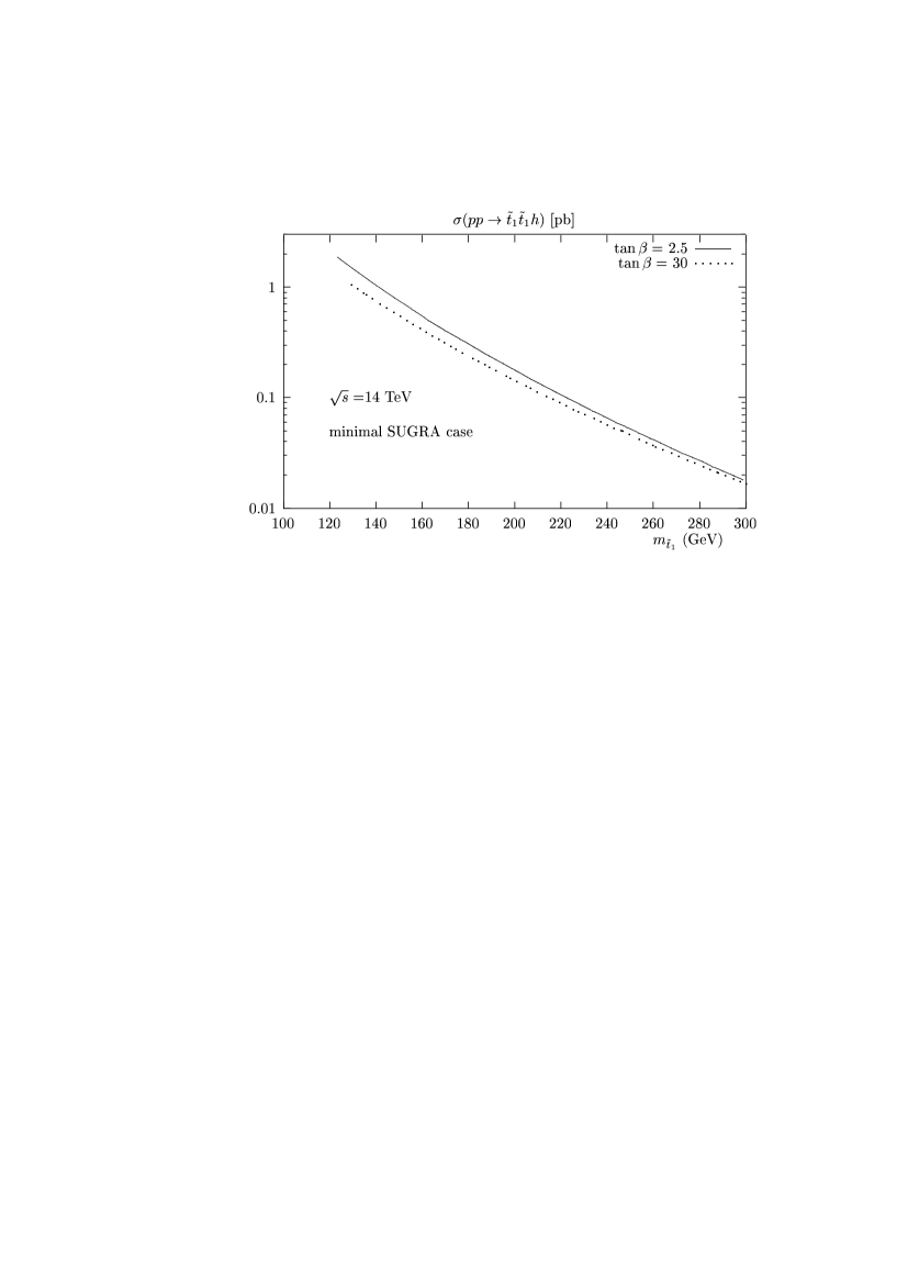
Figure 4: The cross section $\sigma(pp\rightarrow\tilde{t}_{1}\tilde{t}_{1}h$) [in pb] at the LHC as a function of the $\tilde{t}_{1}$ mass in the mSUGRA case: $\tan\beta=2.5(30)$, $m_{1/2}=$ 300 GeV, $A_{0}=-2$ TeV, sign($\mu)=+$.

The mSUGRA cross section as illustrated in Fig. 4 actually corresponds to a situation where $|A_{t}|$ at the relevant electroweak scale is not very large, $|A_{t}|\raisebox{-3.69899pt}{~{}\shortstack{$<$ \\ [-0.07cm] $\sim$}}~{}1$ TeV, while the effective coupling $|\tilde{A}_{t}|$ becomes larger, at least for the small $\tan\beta=$2.5 case, because $\mu$ [which we determine consistently from radiative electroweak symmetry breaking] turns out to be rather large, $\mu\sim 1$ TeV. In this case, for a sufficiently low $m_{\tilde{t}_{1}}$ value the cross section is potentially as large as in the case of the unconstrained MSSM, but this situation clearly occurs in a restricted region of the mSUGRA parameter space. On the other hand, as discussed in subsection 2.2, the mSUGRA case is accordingly less subject to the CCB constraint, since $A_{t}$ is not too large, and also no restrictions are imposed by the $\rho$ parameter until the $\tilde{t}_{1}$ mass becomes really small. However, one should take into account another constraint, namely that of requiring the lightest neutralino [rather than the lightest top squark] to be the lightest SUSY particle (LSP). This is the reason why in Fig. 4 the plots start at $m_{\tilde{t}_{1}}$ values larger than $m_{\chi_{1}^{0}}\sim 120$ GeV, which corresponds to our choice of the basic mSUGRA parameters.

3.2.3 Associated production at the upgraded Tevatron

For completeness, we illustrate some values of the $\tilde{t}_{1}\tilde{t}_{1}h$ production cross section at the upgraded Tevatron with $\sqrt{s}=$ 2 TeV. Naively, one may expect that such a three particle final state process will be very disfavored by phase space in the parton frame, except for a very light $\tilde{t}_{1}$ and very light Higgs bosons which are already excluded by present experimental constraints. However, this clear phase space suppression is partially compensated by the fact that the $q\bar{q}$ hard scattering process [which scales as the inverse of the parton c.m. energy $\hat{s}$] dominates the cross section at the Tevatron. More precisely, due to the fact that Tevatron is a $p\bar{p}$ collider, the cross section benefits form the larger quark/antiquark densities relative to the LHC case.

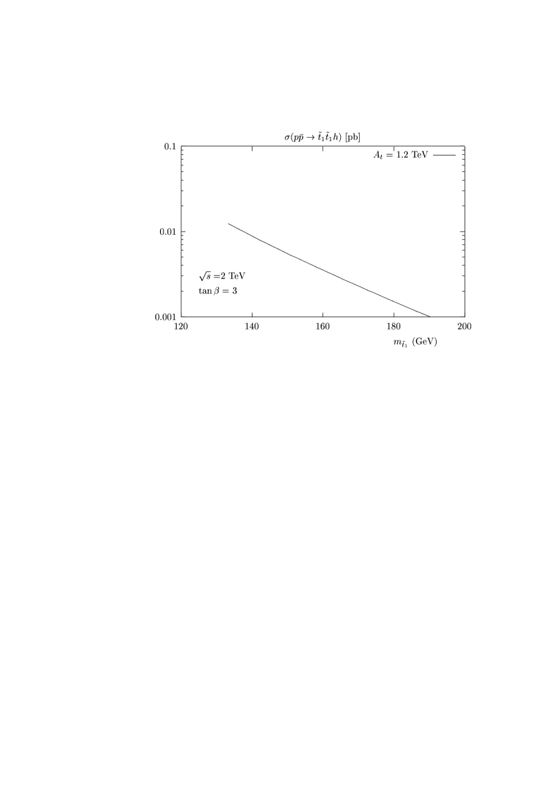
Figure 5: The production cross section $\sigma(p\bar{p}\rightarrow\tilde{t}_{1}\tilde{t}_{1}h$) at the Tevatron [in pb] as a function of the $\tilde{t}_{1}$ mass for $A_{t}=1.2$ TeV, $\mu=-$600 GeV and $\tan\beta=3$.

The cross section $\sigma(p\bar{p}\rightarrow\tilde{t}_{1}\tilde{t}_{1}h$) is shown in Fig. 5 at a c.m. energy $\sqrt{s}=2$ TeV in the case of large $A_{t}$ values, since otherwise the cross section is clearly too small for the process to be relevant. For the planned luminosities of $\int{\cal L}{\rm d}t\sim 10$ fb^-1 [8], one can see from Fig. 5 that up to a few tens of events might be collected for $m_{\tilde{t}_{1}}\sim 130$ GeV [smaller masses for such a large $A_{t}$ value, are already ruled out by the present constraint, as discussed above], before efficiency cuts are applied. This gives some hope that this process might be useful at the Tevatron too. We shall discuss in the next subsection the possible signal for this process, which is similar for the LHC and Tevatron.

3.2.4 Signal

Finally, let us discuss the signal for the $pp\rightarrow\tilde{t}_{1}\tilde{t}_{1}h$ process. If the mass of the lightest top squark is only slightly larger than that of the lightest neutralino [which is expected to be the LSP], the dominant $\tilde{t}_{1}$ decay channel [31] will be the loop induced decay into a charm quark plus a neutralino, $\tilde{t}_{1}\rightarrow c\chi_{1}^{0}$. For larger $m_{\tilde{t}_{1}}$ values, the lightest top squark can decay into a $b$ quark and a chargino, $\tilde{t}_{1}\rightarrow b\chi^{+}$ and possibly into a $t$ quark and the LSP, $\tilde{t}\rightarrow t\chi_{1}^{0}$. [We assume that the strong decay into gluinos does not occur]. In the interesting region where the cross section $\sigma(pp\rightarrow\tilde{t}_{1}\tilde{t}_{1}h)$ is large, i.e. for relatively light $\tilde{t}_{1}$, the decay mode $\tilde{t}_{1}\rightarrow b\chi^{+}$ can be dominant, unless the mass difference $m_{\tilde{t}_{1}}-m_{\chi_{1}^{+}}$ is very small. Assuming that the partners of the leptons are heavier than the lightest chargino, $\chi_{1}^{+}$ will mainly decay into the LSP and a real or virtual $W$ boson, leading to the final state

$$\tilde{t}_{1}\rightarrow bW^{+}\ +\ {\rm missing\ energy}$$ (40)

This is the same topology as in the case of the top quark decay, $t\rightarrow bW^{+}$, except that in the case of the top squark there is a large amount of missing energy due to the undetected LSP. If sleptons are also relatively light, charginos decay will also lead to $l\nu\chi_{1}^{0}$ final states. The only difference between the final states generated by the $\tilde{t}\tilde{t}h$ and $t\bar{t}h$ processes, will be due to the softer energy spectrum of the charged leptons coming from the chargino decay in the former case, because of the energy carried by the invisible neutralinos.

The Higgs boson can be tagged through its $h\rightarrow\gamma\gamma$ decay mode [5]. In the decoupling limit, and for light top squarks and large $\tilde{A}_{t}$ values, the branching ratio for this mode can be enhanced [up to $\sim 20\%$] compared to the $\gamma\gamma$ branching ratio of the SM Higgs boson [13], because of the additional contributions of the $\tilde{t}$–loops which interfere constructively with the dominant $W$–loop contribution.

Although a detailed analysis taking into account backgrounds and detection efficiencies, which is beyond the scope of this paper, will be required to assess the importance of this signal, it is clear that in some areas of the MSSM parameter space, $\gamma\gamma$+ charged lepton events can be much more copious than in the SM, and the contributions of the $pp\rightarrow\tilde{t}\tilde{t}h$ process to these events can render the detection of the $h$ boson much easier than with the process $pp\rightarrow t\bar{t}h$ alone. This excess of events could then allow to measure the $h\tilde{t}_{1}\tilde{t}_{1}$ coupling, and open a window to probe the soft–SUSY breaking parameters of the stop sector. In particular one can obtain some information on the trilinear coupling $A_{t}$, which is rather difficult to extract from the study of the production of SUSY particles at the LHC as shown in Ref. [33].

4. Associated production at e⁺e^- colliders

At future linear $e^{+}e^{-}$ colliders, the final state $\tilde{q}_{1}\tilde{q}_{1}h$ may be generated in three ways: $(i)$ two–body production of a mixed pair of squarks and the decay of the heaviest squark to the lightest one and a Higgs boson [Fig. 6a]; $(ii)$ the continuum production in $e^{+}e^{-}$ annihilation [Fig. 6b]; and $(iii)$ the continuum production in $\gamma\gamma$ collisions [Fig. 6c]. The same picture holds for the associated production of the heavier CP–even Higgs boson $H$ with $\tilde{q}_{1}\tilde{q}_{1}$ pairs. In the case of the pseudoscalar boson $A$ only the processes $(i)$ and $(ii)$ are possible: because of CP–invariance, the coupling $A\tilde{q}_{1}\tilde{q}_{1}$ is absent and the final state $\tilde{q}_{1}\tilde{q}_{1}A$ cannot be generated in $\gamma\gamma$ collisions at tree–level; furthermore, in $e^{+}e^{-}$ annihilation the graph where the $A$ boson is emitted from the $Z$ line is absent, but there is another graph involving the $ZAh(H)$ coupling [see Fig. 6b]. For the associated production of CP–even Higgs bosons with $\tilde{q}_{2}\tilde{q}_{2}$ states, only the processes $(ii)$ and $(iii)$ are relevant.

a)

b)

c)

Figure 6: Feynman diagrams for the production of a Higgs boson $\Phi$ in association with a pair of squarks in $e^{+}e^{-}$ and $\gamma\gamma$ collisions.

4.1 Two–body production and decay

If the center of mass energy of the $e^{+}e^{-}$ collider is high enough, one can generate a $\tilde{q}_{1}\tilde{q}_{1}h$ final state by first producing a mixed pair of squarks, $e^{+}e^{-}\rightarrow\tilde{q}_{1}\tilde{q}_{2}$, through the exchange of a virtual $Z$–boson, and then let the heaviest squark decay into the lightest one and the Higgs boson, $\tilde{q}_{2}\rightarrow\tilde{q}_{1}h$, if the splitting between the two squarks is larger than $M_{h}$; Fig. 6a. For $H$ and $A$ bosons final states, a larger splitting in the stop sector is required.

The total cross section for the production of two squarks with different masses in $e^{+}e^{-}$ annihilation, $e^{+}e^{-}\rightarrow\tilde{q}_{1}\tilde{q}_{2}$, including the factor of two to take into account the charge conjugated states is given by [35]

$$\sigma(e^{+}e^{-}\rightarrow\tilde{q}_{1}\tilde{q}_{2})=\frac{3}{2}\,\sigma_{0}\,(a_{e}^{2}+v_{e}^{2})\,a_{12}^{2}\,\frac{\lambda^{3/2}(s,m_{\tilde{q}_{1}}^{2},m_{\tilde{q}_{2}}^{2})}{s(s-M_{Z}^{2})^{2}}$$ (41)

with $s$ the center of mass energy of the $e^{+}e^{-}$ collider; $\sigma_{0}=4\pi\alpha^{2}/3s$ the QED point cross section and $\lambda$ the usual two–body phase–space function, $\lambda(x,y,z)=x^{2}+y^{2}+z^{2}-2(xy+xz+yz)$. The $Z\tilde{q}_{1}\tilde{q}_{2}$ coupling $a_{12}$ is proportional to $\sin 2\theta_{q}$, eq. (15), and in the case where the mixing between squarks is absent, this coupling is zero and the cross section vanishes. [The QCD corrections to this process, including the SUSY–QCD contributions with the exchange of gluinos, are available [36] and can be included.]

The partial decay width of the heaviest squark into the lightest squark and a neutral Higgs boson $\Phi=h,H,A$ is given by [35]

$$\Gamma(\tilde{q}_{2}\rightarrow\tilde{q}_{1}\Phi)=\frac{G_{F}M_{Z}^{4}}{2\sqrt{2}\pi\,m_{\tilde{q}_{2}}^{3}}\,\lambda^{1/2}(m_{\tilde{q}_{2}}^{2},M_{\Phi}^{2},m_{\tilde{q}_{1}}^{2})\;g^{2}_{\Phi\tilde{q}_{1}\tilde{q}_{2}}$$ (42)

where the two–body phase space function $\lambda$ has been given previously. [Here also the QCD corrections are available [37] and can be included]. As can be seen from inspection of eq. (22), in contrast with the $g_{\Phi\tilde{q}_{1}\tilde{q}_{1}}$ coupling, $|g_{\Phi\tilde{q}_{1}\tilde{q}_{2}}|$ cannot be too large in most of the parameter space, and in fact this coupling is well dominated by its second term, proportional to $\cos 2\theta_{q}$, except for very large $\tilde{A}_{t}$ and/or when the mixing between squarks is maximal, $|\theta_{q}|=\pi/4$, in which case it is anyway practically vanishing.

The branching ratio for the $\tilde{q}_{2}\rightarrow\tilde{q}_{1}\Phi$ decay mode is obtained by dividing the partial width by the total $\tilde{q}_{2}$ decay width. The latter is obtained by summing the widths of all possible decay channels. For instance, in the case of the more phase–space favored decay channel $\tilde{t}_{2}\rightarrow\tilde{t}_{1}h$, one has to include: decays of the $\tilde{t}_{2}$ into a bottom squark and a charged Higgs or $W$ boson, decays into $\tilde{t}_{1}$ and a neutral Higgs or $Z$ boson, decays into a $b$ quark and charginos, and decays into a top quark and neutralinos [or gluinos].

In principle, if phase–space allowed, the cross section for the two–body production process times the branching ratio for the two–body decay, should be large enough for the final state to be copiously produced. However, as discussed above, in a large part of the parameter space the cross section times branching ratio will be roughly proportional to $\sin 2\theta_{q}\times\cos 2\theta_{q}$, thus giving small production rates in the no mixing and maximal mixing scenarii. In addition, the decay width $\tilde{q}_{2}\rightarrow h\tilde{q}_{1}$ is in general much smaller than the $\tilde{q}_{2}$ decay widths into chargino and neutralinos, leading to a small branching ratio. Nevertheless, there are regions of the MSSM parameter space where the combination $\sin 2\theta_{q}\times\cos 2\theta_{q}$ can be maximal, which occurs typically for a not too small $m_{\tilde{t}_{L}}$–$m_{\tilde{t}_{R}}$ splitting and a moderate $\tilde{A}_{t}$, as can be seen from eq. (8). In this case [which is often realized in particular in the mSUGRA case, as we shall discuss next] the resonant $\tilde{t}_{2}$ process may dominate over the non-resonant $\tilde{q}\tilde{q}h$ production and the corresponding rate is visible for the high luminosities $\int{\cal L}{\rm d}t\sim 500$ fb^-1 expected at linear colliders [38].

Such a situation is illustrated in the case of the $\tilde{t}_{1}\tilde{t}_{1}h$ final state in Fig. 7, where the cross section $e^{+}e^{-}\rightarrow\tilde{t}_{1}\tilde{t}_{2}$ times the branching ratio BR($\tilde{t}_{2}\rightarrow\tilde{t}_{1}h)$ is shown as a function of the $\tilde{t}_{1}$ mass at a c.m. energy of $\sqrt{s}=800$ GeV [full lines]. We have chosen a mSUGRA scenario with $\tan\beta=30$, $m_{1/2}=$ 100 GeV, $A_{0}=-600$ GeV and sign$(\mu)=+$. [The broken lines show the contribution of the non–resonant contributions in this case, which will be discussed in more detail later]. As can be seen, the cross section can reach the level of 1 fb for relatively small $m_{\tilde{t}_{1}}$ values, leading to more than one thousand events in the course of a few years, with the expected integrated luminosity of $\int{\cal L}{\rm d}t\sim 500$ fb^-1 [38]. Moreover, for the same reasons that have been discussed in previous $pp$ section for the mSUGRA case, there are no other constraints e.g. from CCB or the rho parameter, for the values chosen in our illustration.

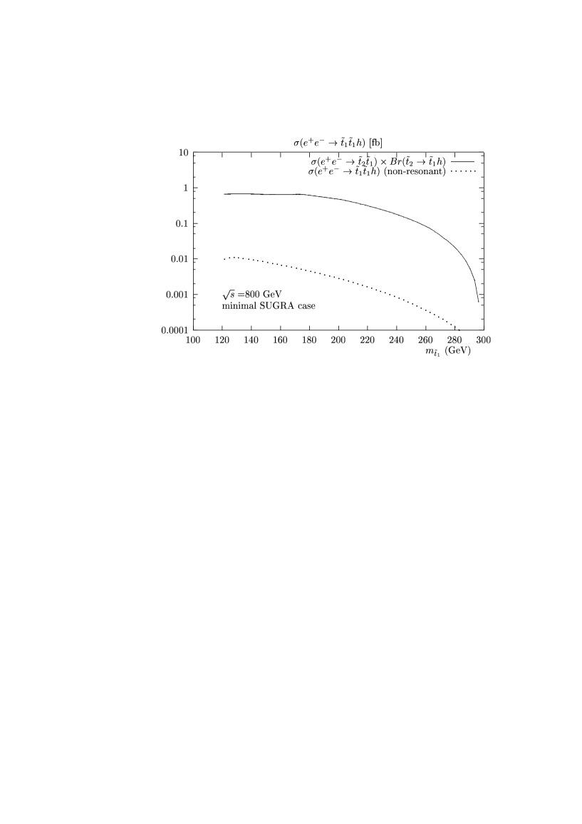
Figure 7: The production cross section $\sigma(e^{+}e^{-}\rightarrow\tilde{t}_{1}\tilde{t}_{1}h$) [in fb] as a function of $m_{\tilde{t}_{1}}$ in the mSUGRA case; $\tan\beta=$ 30, $m_{1/2}=$ 100 GeV and $A_{0}=-600$ GeV.

As discussed in the previous section the top squarks in this mass range will mainly decay into a charm+neutralino, $\tilde{t}_{1}\to c\chi_{1}^{0}$, or a $b$ quark and a chargino, $\tilde{t}_{1}\rightarrow b\chi^{+}$. In this latter case the lightest chargino, $\chi_{1}^{+}$ will decay into the LSP and a real or virtual $W$ boson, leading to the same topology as in the case of the top quark decay, but with a large amount of missing energy due to the undetected LSP. However, in $e^{+}e^{-}$ collisions one can use the dominant decay mode of the lightest Higgs boson, $h\rightarrow b\bar{b}$. The final state topology will consist then of $4b$ quarks [two of them peaking at an invariant mass $M_{h}$, which would be already measured by means of another process], two [real or virtual] $W$’s and missing energy. With the help of efficient micro–vertex detectors, this spectacular final state should be rather easy to detect in the clean environment of $e^{+}e^{-}$ colliders.

4.2 Production in the continuum in e⁺e^- collisions

There are three types of Feynman diagrams leading to final states with $\tilde{q}_{1}\tilde{q}_{1}$ pairs and a CP–even Higgs boson $h$ or $H$, in $e^{+}e^{-}$ annihilation: Higgs boson emission from the $\tilde{q}_{1}$ states [which are produced through s–channel photon and $Z$–boson exchange], Higgs boson emission from the $\tilde{q}_{2}$ state [which is produced with $\tilde{q}_{1}$ through $Z$–boson exchange], and Higgs boson emission from a virtual $Z$ boson which then splits into $\tilde{q}_{1}\tilde{q}_{1}$ pairs. When the Higgs–$\tilde{q}_{1}\tilde{q}_{1}$ couplings are large, the two last types of Feynman diagrams give negligible contributions since the virtuality of $\tilde{q}_{2}$ is large and the $Z\tilde{q}_{1}\tilde{q}_{1}$ coupling not enhanced. [In the opposite situation where the squark mixing angle $\theta_{q}$ is non-zero but moderate, when the (resonant) $\tilde{q}_{2}$ contribution largely dominates the cross section, it is then very well approximated by the on–shell $\tilde{q}_{1}\tilde{q}_{2}$ production with subsequent decay $\tilde{q}_{2}\to\tilde{q}_{1}h$, as illustrated in the previous subsection 4.1 in the mSUGRA case]. For the CP–odd Higgs boson the first and last possibilities are absent because of CP–invariance which forbids the couplings of $A$ to gauge bosons and $\tilde{q}_{1}\tilde{q}_{1}$ pairs.

Let us first discuss the process $e^{+}e^{-}\rightarrow\tilde{q}_{i}\tilde{q}_{i}\Phi$ with $\Phi$ the CP–even Higgs boson $h$ or $H$, and $\tilde{q}_{i}$ any of the two squarks. In terms of the scaled energies of the two final state squarks $x_{1,2}=2E_{1,2}/\sqrt{s}$, the Dalitz plot density for the reaction reads

$$\frac{{\rm d}\sigma}{{\rm d}x_{1}x_{2}}(e^{+}e^{-}\rightarrow\tilde{q}_{i}\tilde{q}_{i}\Phi)=\sigma_{0}\frac{\alpha N_{c}}{16\pi s_{W}^{2}c_{W}^{2}}\,z\,\sum_{k=1,6}A_{k}$$ (43)

Using the reduced masses $\mu_{i}=m_{\tilde{q}_{i}}^{2}/s,\mu_{j}=m_{\tilde{q}_{j}}^{2}/s$ [$\tilde{q}_{j}$ is the virtually exchanged partner of the produced squark $\tilde{q}_{i}$], $\mu_{\Phi}=M_{\Phi}^{2}/s$ and $z=M_{Z}^{2}/s$, and the couplings given in section 2, the various amplitudes squared are as follows:

$$A_{1} = \left[e_{e}^{2}e_{t}^{2}+2\frac{e_{e}e_{t}v_{e}a_{ii}}{1-z}+\frac{(a_{e}^{2}+v_{e}^{2})a_{ii}^{2}}{(1-z)^{2}}\right]g^{2}_{\Phi\tilde{q}_{i}\tilde{q}_{i}}\left[\frac{2y_{1}-1+4\mu_{i}}{y_{1}^{2}}-\frac{y_{1}+y_{2}-1+2x_{\Phi}}{y_{1}y_{2}}\right.$$

$$+y_{1}\leftrightarrow y_{2}\bigg{]}$$

$$A_{2} = 2\left[\frac{e_{e}e_{t}v_{e}a_{ij}}{1-z}+\frac{(a_{e}^{2}+v_{e}^{2})a_{ii}a_{ij}}{(1-z)^{2}}\right]g_{\Phi\tilde{q}_{i}\tilde{q}_{j}}g_{\Phi\tilde{q}_{i}\tilde{q}_{i}}\left[\frac{2y_{1}-1+4\mu_{i}}{y_{1}(y_{1}+\mu_{i}-\mu_{j})}-\frac{y_{1}+y_{2}-1+2x_{\Phi}}{y_{1}(y_{2}+\mu_{i}-\mu_{j})}\right.$$

$$+y_{1}\leftrightarrow y_{2}\bigg{]}$$

$$A_{3} = \frac{(a_{e}^{2}+v_{e}^{2})a_{ij}^{2}}{(1-z)^{2}}\,g^{2}_{\Phi\tilde{q}_{i}\tilde{q}_{j}}\left[\frac{2y_{1}-1+4\mu_{i}}{(y_{1}+\mu_{i}-\mu_{j})^{2}}-\frac{y_{1}+y_{2}-1+2x_{\Phi}}{(y_{1}+\mu_{i}-\mu_{j})(y_{2}+\mu_{i}-\mu_{j})}+y_{1}\leftrightarrow y_{2}\right]$$

$$A_{4} = \left[\frac{e_{e}e_{t}v_{e}a_{ii}g_{\Phi}}{1-z}+\frac{(a_{e}^{2}+v_{e}^{2})\,a_{ii}^{2}\,g^{2}_{\Phi}}{(1-z)^{2}}\right]g_{\Phi\tilde{q}_{i}\tilde{q}_{i}}\left[\frac{4\mu_{i}-2x_{\Phi}+y_{1}-y_{2}}{y_{1}(x_{\Phi}+2\mu_{i}-z)}+y_{1}\leftrightarrow y_{2}\right]$$

$$A_{5} = \frac{(a_{e}^{2}+v_{e}^{2})a_{ii}a_{ij}g_{\Phi}}{(1-z)^{2}}\,g_{\Phi\tilde{q}_{i}\tilde{q}_{j}}\left[\frac{4\mu_{i}-2x_{\Phi}+y_{1}-y_{2}}{(y_{1}+\mu_{i}-\mu_{j})(x_{\Phi}+2\mu_{i}-z)}+y_{1}\leftrightarrow y_{2}\right]$$

$$A_{6} = \frac{(a_{e}^{2}+v_{e}^{2})a_{ii}^{2}g^{2}_{\Phi}}{(1-z)^{2}}\frac{2\mu_{i}-x_{\Phi}}{(x_{\Phi}+2\mu_{i}-z)^{2}}$$ (44)

In these equations, $y_{1,2}=1-x_{1,2}$, $x_{\Phi}=1-y_{1}-y_{2}+\mu_{\Phi}-2\mu_{i}$ and the (reduced) couplings $g_{\Phi}$ of the $\Phi$ boson to two $Z$ bosons [in units of $eM_{Z}/(s_{W}c_{W})$] are given by: $g_{h}=\sin(\beta-\alpha)$ and $g_{H}=\cos(\beta-\alpha)$.

For the final state $\Phi\tilde{q}_{1}\tilde{q}_{1}$ in the case where the $g_{\Phi\tilde{q}_{1}\tilde{q}_{1}}$ coupling is large [leading to a large splitting between the $\tilde{q}_{1}$ and $\tilde{q}_{2}$ states], the virtuality of the squark $\tilde{q}_{2}$ is large and the $Z\tilde{q}_{1}\tilde{q}_{1}$ coupling not enhanced; the Dalitz plot density of the process can be then approximated by the very simple form

$$\frac{{\rm d}\sigma}{{\rm d}x_{1}x_{2}}(e^{+}e^{-}\rightarrow\tilde{q}_{1}\tilde{q}_{1}\Phi) = \sigma_{0}\frac{\alpha N_{c}}{16\pi s_{W}^{2}c_{W}^{2}}\,z\left[e_{e}^{2}e_{t}^{2}+2\frac{e_{e}e_{t}v_{e}a_{ii}}{1-z}+\frac{(a_{e}^{2}+v_{e}^{2})a_{ii}^{2}}{(1-z)^{2}}\right]g^{2}_{\Phi\tilde{q}_{i}\tilde{q}_{i}}$$ (45)

$$\times \left[\frac{2y_{1}-1+4\mu_{i}}{y_{1}^{2}}-\frac{y_{1}+y_{2}-1+2x_{\Phi}}{y_{1}y_{2}}+y_{1}\leftrightarrow y_{2}\right]$$

For the associated production of the pseudoscalar Higgs boson with a pair of squarks, $e^{+}e^{-}\rightarrow\tilde{q}_{i}\tilde{q}_{i}A$, the Dalitz plot density has a much simpler form since only the diagrams with the virtual $\tilde{q}_{j}$ exchange and the one involving the $ZAh(H)$ vertices, are present. It reads:

$$\frac{{\rm d}\sigma}{{\rm d}x_{1}x_{2}}(e^{+}e^{-}\rightarrow\tilde{q}_{i}\tilde{q}_{i}A)=\sigma_{0}\frac{\alpha N_{c}}{16\pi s_{W}^{2}c_{W}^{2}}\,z\,\frac{(a_{e}^{2}+v_{e}^{2})}{(1-z)^{2}}\,\sum_{k=1,3}B_{k}$$ (46)

where the amplitudes squared, using the same notation as previously, are given by

$$B_{1} = a_{ij}^{2}g^{2}_{A\tilde{q}_{i}\tilde{q}_{j}}\left[\frac{2y_{1}-1+4\mu_{i}}{(y_{1}+\mu_{i}-\mu_{j})^{2}}-\frac{y_{1}+y_{2}-1+2x_{A}}{(y_{1}+\mu_{i}-\mu_{j})(y_{2}+\mu_{i}-\mu_{j})}+y_{1}\leftrightarrow y_{2}\right]$$

$$B_{2} = (1-2y_{1}-2y_{2}+4\mu_{A})\left[\frac{g_{ZAh}g_{h\tilde{q}_{i}\tilde{q}_{i}}}{x_{A}+2\mu_{i}-\mu_{h}}+\frac{g_{ZAH}g_{H\tilde{q}_{i}\tilde{q}_{i}}}{x_{A}+2\mu_{i}-\mu_{H}}\right]^{2}$$

$$B_{3} = -2g_{A\tilde{q}_{i}\tilde{q}_{j}}a_{ij}\left[\frac{g_{ZAh}g_{h\tilde{q}_{i}\tilde{q}_{i}}}{x_{A}+2\mu_{i}-\mu_{h}}+\frac{g_{ZAH}g_{H\tilde{q}_{i}\tilde{q}_{i}}}{x_{A}+2\mu_{i}-\mu_{H}}\right]$$ (47)

$$\times\left[\frac{y_{1}-2\mu_{A}}{(y_{1}+\mu_{i}-\mu_{j})}-y_{1}\leftrightarrow y_{2}\right]$$

with the $Z\Phi A$ couplings $g_{ZAh}=\cos(\beta-\alpha)/(2s_{W}c_{W})$ and $g_{ZAH}=-\sin(\beta-\alpha)/(2s_{W}c_{W})$ (in units of $e$); here again $\tilde{q}_{j}$ is the virtually exchanged partner of the produced squark $\tilde{q}_{i}$ with $\tilde{q}_{j}\neq\tilde{q}_{i}$.

To obtain the total production cross section $\sigma(e^{+}e^{-}\rightarrow\tilde{q}_{i}\tilde{q}_{i}\Phi)$, one has to integrate over the scaled variables $x_{1,2}\equiv 2E_{1,2}/\sqrt{s}$ in a way totally similar to the one described in previous section 3, see eqs. (35–38).

Figure 8: The cross section $\sigma(e^{+}e^{-}\rightarrow\tilde{t}_{1}\tilde{t}_{1}h$) [in fb] as a function of the $\tilde{t}_{1}$ mass and three different choices of the other parameters: $\tan\beta=30$, $A_{t}=$ 0 (0.5) TeV; $\tan\beta=3$, $A_{t}=$ 1.2 TeV.

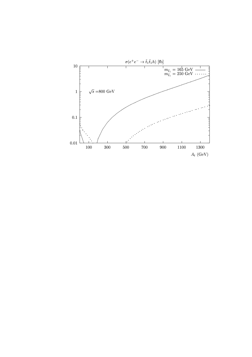
Figure 9: The cross section $\sigma(e^{+}e^{-}\rightarrow\tilde{t}_{1}\tilde{t}_{1}h$) [in fb] as a function of $A_{t}$ for fixed $m_{\tilde{t}_{1}}=165$ ($\tan\beta=3$); and 250 GeV ($\tan\beta=30)$.

To illustrate the magnitude of the cross sections, we show in Figs. 8–9 the rates for the $\tilde{t}_{1}\tilde{t}_{1}h$ final state in the decoupling limit at $\sqrt{s}=800$ GeV and $\tan\beta=30(3)$ as a function of the $\tilde{t}_{1}$ mass for $A_{t}\simeq 0$ and $A_{t}=0.5$ TeV ($A_{t}=1.2$ TeV) respectively [Fig. 8], and as a function of $A_{t}$ for $m_{\tilde{t}_{1}}=$ 165 GeV ($\tan\beta=3$), and 250 GeV ($\tan\beta=30$) [Fig. 9], i.e. for the same scenarii as in Figs. 2 and 3 of section 3 [the discussions on the constraints on the parameters $A_{t}$ and $m_{\tilde{t}_{1}}$ given there apply also in this case].

As can be seen the trend is similar to the one discussed in the previous section for the associated production at proton colliders. For not too large $\tilde{t}_{1}$ masses and large values of the parameter $\tilde{A}_{t}$, the production cross sections can exceed the value $\sigma(e^{+}e^{-}\rightarrow\tilde{t}_{1}\tilde{t}_{1}h)\sim 1$ fb. [Note that the cross section for the SM–like process $e^{+}e^{-}\rightarrow t\bar{t}h$ [18] is of the order of 2 fb for $M_{h}\sim 130$ GeV at a c.m. energy $\sqrt{s}=800$ GeV.] This provides more than one thousand events in a few years, with a luminosity $\int{\cal L}{\rm d}t\sim 500$ fb^-1: a sample which should be sufficient to isolate the final state [with the topologies discussed in section 4.1] and measure the $g_{\tilde{t}_{1}\tilde{t}_{1}h}$ coupling with some accuracy.

At lower energies, the production cross section will be as large as in the previous case for small $\tilde{t}_{1}$ masses, but will be limited by phase space for larger values. This is illustrated in Fig. 10, with the same choice of parameters as in Fig. 8, but with a c.m. energy of $\sqrt{s}=500$ GeV. Thus for very large values of $A_{t}$, the cross section $\sigma(e^{+}e^{-}\rightarrow\tilde{t}_{1}\tilde{t}_{1}h$) can exceed the fb level for stop masses below $m_{\tilde{t}_{1}}\raisebox{-3.69899pt}{~{}\shortstack{$<$ \\ [-0.07cm] $\sim$}}~{}150$ GeV even at a 500 GeV collider. With $\sim 500$ fb^-1 luminosity, this would hopefully allow to detect the final state and measure the coupling $g_{h\tilde{t}_{1}\tilde{t}_{1}}$ with some accuracy. In the mSUGRA case the cross section generally follows also the same lines as in section 3.2.2 and Fig. 4, i.e. it can be as large as in the case of the unconstrained MSSM, but in relatively smaller area of the SUSY parameter space, for reasons that have been given earlier.

Figure 10: Same as Fig. 8 but with $\sqrt{s}=500$ GeV.

Note finally that in the unconstrained MSSM case, the continuum production cross section in $e^{+}e^{-}$ annihilation $\sigma(e^{+}e^{-}\rightarrow\tilde{t}_{1}\tilde{t}_{1}h$) is often larger than the resonant cross section for the production of $\tilde{t}_{1}\tilde{t}_{2}$ and the subsequent 2–body decay $\tilde{t}_{2}\rightarrow\tilde{t}_{1}h$, but this is not generic. Indeed, in a situation where both a non-negligible $m_{\tilde{t}_{L}}$–$m_{\tilde{t}_{R}}$ splitting and a moderate $\tilde{A}_{t}$ occurs, provided there is sufficient phase space allowed, the production via a resonant $\tilde{t}_{2}$ becomes competitive and even dominant, as illustrated in a typical mSUGRA case in the previous subsection 4.1.

4.3. Production in the continuum in $\gamma\gamma$ collisions

Future high–energy $e^{+}e^{-}$ linear colliders can be turned into high–energy $\gamma\gamma$ colliders, with the high energy photons coming from Compton back–scattering of laser beams. The c.m. energy of the $\gamma\gamma$ collider is expected to be as much as $\sim 80\%$ of the one of the original $e^{+}e^{-}$ machine. However, the total luminosity is expected to be somewhat smaller than the one of the $e^{+}e^{-}$ mode, leading to a smaller number of events for the same cross section.

The final state $\tilde{q}_{i}\tilde{q}_{i}h$ or $H$ can be generated by emitting the $h,H$ bosons from the squark lines in the process $\gamma\gamma\rightarrow\tilde{q}_{i}\tilde{q}_{i}$; Fig. 6c. The pseudoscalar Higgs boson $A$ cannot be produced in two–photon collisions in association with a pair of squarks because of CP–invariance; the production of the $A$ boson is only possible in association with $\tilde{q}_{1}\tilde{q}_{2}$ states which is less favored by phase space.

The differential cross section of the subprocess $\gamma\gamma\rightarrow\tilde{q}_{i}\tilde{q}_{i}\Phi$ with $\Phi$ a CP–even Higgs boson is given by

$$d\sigma(\gamma\gamma\rightarrow\tilde{q}_{i}\tilde{q}_{i}\Phi)=\frac{1}{2s}\times d{\rm PS}\times|M|^{2}_{\gamma\gamma}$$ (48)

where dPS is the same element of the 3–body phase space discussed in section 3 for hadron colliders, and $|M|^{2}_{\gamma\gamma}$ is the amplitude squared of the subprocess; taking the same convention as in section 3 for the momenta of the initial and final particles, and averaging over spin, the latter is given by

$$|M|^{2}_{\gamma\gamma}=\frac{1}{4}\,e_{q}^{4}\,(4\sqrt{2}\;G_{F}\;M_{Z}^{4}\;g^{2}_{\Phi\tilde{q}_{i}\tilde{q}_{i}}\;e^{4})\left[g_{1}+g_{2}A_{1}+g_{3}A_{2}+g_{4}A_{1}A_{2}+g_{5}A_{1}^{2}+g_{6}A_{2}^{2}\right]$$ (49)

where $A_{1,2}$ have been defined in eq. (19); in terms of the variables $y_{1,2},x,y$ defined also in eq. (19), and ${s},m_{\tilde{q}_{i}}$ the c.m. energy of the $\gamma\gamma$ subprocess and the squark mass respectively, the coefficients $g_{i}$ read:

$$g_{1} = \frac{1}{{s}^{2}y_{1}y_{2}}\bigg{[}2(p_{1}.p_{2}{s}-2x)^{2}+\frac{(m_{\tilde{q}_{i}}^{2}{s}-4y_{1})(m_{\tilde{q}_{i}}^{2}{s}-4y_{2})(x^{2}-2y_{1}y_{2})}{y_{1}y_{2}}\bigg{]}$$

$$g_{2} = \frac{1}{{s}^{2}y_{1}y_{2}^{2}}\bigg{[}4(p_{1}.p_{2}{s}-2x)x(-m_{\tilde{q}_{i}}^{2}p_{2}.q_{+}{s}+(4p_{2}.q_{+}+{s})y_{2})\bigg{]}$$

$$g_{3} = \frac{1}{{s}^{2}y_{1}^{2}y_{2}}\bigg{[}4(p_{1}.p_{2}{s}-2x)x(m_{\tilde{q}_{i}}^{2}p_{1}.q_{+}{s}+(-4p_{1}.q_{+}+{s})y_{1})\bigg{]}$$

$$g_{4} = \frac{8}{{s}^{2}y_{1}y_{2}}\bigg{[}-(p_{1}.q_{+}p_{2}.q_{+}(p_{1}.p_{2}{s}-2x)^{2})$$

$$+{s}(-2y_{1}y_{2}(2(p_{1}.q_{+}-p_{2}.q_{+})-{s})-m_{\tilde{q}_{i}}^{2}{s}(p_{2}.q_{+}y_{1}-p_{1}.q_{+}y_{2}))\bigg{]}$$

$$g_{5} = 4\bigg{[}2+\frac{p_{2}.q_{+}(m_{\tilde{q}_{i}}^{2}{s}-4y_{2})(m^{2}_{\tilde{q}_{i}}p_{2}\cdot q_{+}{s}-2y_{2}(2p_{2}.q_{+}+{s}))}{{s}^{2}y_{2}^{2}}\bigg{]}$$

$$g_{6} = 4\bigg{[}2+\frac{p_{1}.q_{+}(m_{\tilde{q}_{i}}^{2}{s}-4y_{1})(m_{\tilde{q}_{i}}^{2}p_{1}.q_{+}{s}+2y_{1}(-2p_{1}.q_{+}+{s}))}{{s}^{2}y_{1}^{2}}\bigg{]}$$ (50)

Integrating over the phase–space in a similar way as the one discussed in section 3, one obtains the total production cross section of this subprocess. One can then convolute with the photon spectra [some examples of spectra can be found in Ref. [39] for instance] to obtain the final cross section $\sigma(\gamma\gamma\rightarrow\tilde{q}_{i}\tilde{q}_{i}\Phi)$. In the following, we will not use any photon spectrum for simplicity, we will just exhibit and discuss the production cross section for the subprocess.

The total cross section for the process $\gamma\gamma\rightarrow\tilde{t}_{1}\tilde{t}_{1}h$ is shown in Fig. 11 at a two–photon c.m. energy $\sqrt{s}_{\gamma\gamma}\raisebox{-3.69899pt}{~{}\shortstack{$<$ \\ [-0.07cm] $\sim$}}~{}0.8\sqrt{s}_{ee}=600$ GeV and as a function of the $\tilde{t}_{1}$ mass, without convolution with the photon spectrum and with the same inputs and assumptions as in Fig. 8 to compare with the $e^{+}e^{-}$ mode. Because the c.m. energy of the $\gamma\gamma$ collider is only $\sim 80\%$ of the one of the original $e^{+}e^{-}$ machine, the process is of course less phase–space favored than in the $e^{+}e^{-}$ mode. Nevertheless, the cross section for the $\tilde{t}_{1}\tilde{t}_{1}h$ final state is of the same order as in the $e^{+}e^{-}$ mode for c.m. energies not too close to the kinematical threshold, and the process might be useful to obtain complementary information since it does not involve the $Z$–boson and $\tilde{t}_{2}$ exchanges. If the luminosities of the $\gamma\gamma$ and $e^{+}e^{-}$ colliders are comparable, a large number of events might be collected for small stop masses and large $A_{t}$ values.

Figure 11: The cross section $\sigma(\gamma\gamma\rightarrow\tilde{t}_{1}\tilde{t}_{1}h$) in $\gamma\gamma$ collisions [in fb] at a center of mass energy $\sqrt{s_{\gamma\gamma}}=600$ GeV as a function of $m_{\tilde{t}_{1}}$. The other parameters have the same values as in Fig. 10.

5. Conclusions

We have calculated the cross sections for the production of neutral Higgs particles in association with the supersymmetric scalar partners of the third generation quarks, $e^{+}e^{-}\rightarrow\tilde{q}_{i}\tilde{q}_{i}\Phi$, at future high–energy hadron colliders and at $e^{+}e^{-}$ linear machines, in both the $e^{+}e^{-}$ annihilation and the $\gamma\gamma$ fusion mode. Complete but rather simple analytical formulae for the squared amplitudes of these three–body processes are given in the case where the two final state squarks have equal mass. In the case of $e^{+}e^{-}$ collisions, the production of both the CP–even and CP–odd Higgs bosons were calculated, while in $pp$ and $\gamma\gamma$ collisions only the production of the CP–even Higgs particles has been discussed, since pseudoscalar Higgs bosons cannot be produced at tree–level with a pair of equal mass squarks at these colliders.

In the framework of the Minimal Supersymmetric extension of the Standard Model, we have then investigated the magnitude of the cross sections at the upgraded Tevatron and the LHC for hadron machines, and at a future $e^{+}e^{-}$ linear machine with c.m. energies in the range $\sqrt{s}=$500–800 GeV; in the latter case, the $\gamma\gamma$ option of the collider has also been considered. In this numerical analysis, we focussed on the production of the lightest CP–even Higgs boson in the decoupling regime, in association with a pair of the lightest top squarks. Final states with the other Higgs bosons or with $\tilde{q}_{1}\tilde{q}_{2}$ pairs should be phase–space suppressed.

At the LHC, the production cross sections can be rather substantial, especially in the case of rather light top squarks, $m_{\tilde{t}_{1}}\raisebox{-3.69899pt}{~{}\shortstack{$<$ \\ [-0.07cm] $\sim$}}~{}250$ GeV and large trilinear coupling $\tilde{A}_{t}\raisebox{-3.69899pt}{~{}\shortstack{$>$ \\ [-0.07cm] $\sim$}}~{}1$ TeV. In this case the production rates can exceed the one for the standard–like production of the $h$ boson in association with top quarks, $pp\rightarrow t\bar{t}h$, which is expected to provide a signal of the $h$ boson in the $\gamma\gamma l^{\pm}$ channel. Although a detailed Monte-Carlo analysis, which is beyond the scope of this paper, will be required to assess the importance of this signal and to optimize the cuts needed not to dilute the contribution of the $\tilde{t}_{1}\tilde{t}_{1}h$ final states, it turns out that in a substantial area of the MSSM parameter space, the contribution of the top squark to the $\gamma\gamma l^{\pm}$ signal can significantly enhance the potential of the LHC to discover the lightest MSSM Higgs boson in this channel.

At $e^{+}e^{-}$ colliders with c.m. energies around $\sqrt{s}=800$ GeV and with very high luminosities $\int{\cal L}{\rm d}t\sim 500$ fb^-1, the process $e^{+}e^{-}\rightarrow\tilde{t}_{1}\tilde{t}_{1}h$ can lead to several hundreds of events, since the cross sections [in particular for rather light top squarks, $m_{\tilde{t}_{1}}\raisebox{-3.69899pt}{~{}\shortstack{$<$ \\ [-0.07cm] $\sim$}}~{}250$ GeV and large trilinear coupling, $\tilde{A}_{t}\raisebox{-3.69899pt}{~{}\shortstack{$>$ \\ [-0.07cm] $\sim$}}~{}1$ TeV] can exceed the level of a 1 fb, and thus the rate for the standard–like process $e^{+}e^{-}\rightarrow t\bar{t}h$. In the case where the top squark decays into a $b$ quark and a real/virtual chargino, the final state topology [with $4b$ quarks, missing energy and additional jets or leptons] will be rather spectacular and should be easy to be seen experimentally, thanks to the clean environment of these colliders. In the $\gamma\gamma$ option of the $e^{+}e^{-}$ collider, the cross sections are similar as previously far from the particle thresholds, but are suppressed for larger masses because of the reduced c.m. energies. For $\gamma\gamma$ luminosities of the same order as the original $e^{+}e^{-}$ luminosities, the $\tilde{t}_{1}\tilde{t}_{1}h$ final state should also be observable in the two–photon mode, at least in some areas of the MSSM parameter space.

The production cross section of the $\tilde{t}_{1}\tilde{t}_{1}h$ final state is directly proportional to the square of the $\tilde{t}_{1}\tilde{t}_{1}h$ couplings, the potentially largest electroweak coupling in the MSSM. Analyzing these final states at hadron or electron–positron machines will therefore allow to measure this coupling, opening thus a window to probe directly some of the soft–SUSY breaking scalar potential.

Acknowledgements:

We thank M. Drees and M. Spira for discussions, and D. Denegri and E. Richter–Was for their interest in this problem. This work has been performed in the framework of the “GDR–Supersymétrie”; discussions with some members of the GDR are acknowledged.

References

- [1] For reviews on Supersymmetry and the MSSM see: H. P. Nilles, Phys. Rep. 117 (1985) 1; P. Nath, R. Arnowitt and A. Chamseddine, Applied N=1 Supergravity, ICTP series in Theoretical Physics, World Scientific, Singapore, 1984; Haber and G. Kane, Phys. Rep. 117 (1985) 75.
- [2] For a review on the MSSM Higgs sector, see J.F. Gunion, H.E. Haber, G.L. Kane and S. Dawson, The Higgs Hunter’s Guide, Addison–Wesley, Reading 1990.
- [3] Y. Okada, M. Yamaguchi and T. Yanagida, Prog. Theor. Phys. 85 (1991) 1; H. Haber and R. Hempfling, Phys. Rev. Lett. 66 (1991) 1815; J. Ellis, G. Ridolfi and F. Zwirner, Phys. Lett. 257B (1991) 83; R. Barbieri, F. Caravaglios and M. Frigeni, Phys. Lett. 258B (1991) 167.
- [4] M. Carena, M. Quiros and C.E.M. Wagner, Nucl. Phys. B461 (1996) 407; H. Haber, R. Hempfling and A. Hoang, Z. Phys. C75 (1997) 539; S. Heinemeyer, W. Hollik and G. Weiglein, hep–ph/9803277.
- [5] ATLAS Collaboration, Technical Proposal, Report CERN–LHCC 94–43; CMS Collaboration, Technical Proposal, Report CERN–LHCC 94–38.
- [6] E. Accomando et al., LC CDR Report DESY 97-100 Physics Reports 299 (1998) 1; S. Kuhlman et al., NLC ZDR Design Group and the NLC Physics Working Group, report SLAC–R–0485.
- [7] M. Carena, P.M. Zerwas et al., “Higgs Physics at LEP2”, CERN Yellow Report CERN-96-01, hep–ph/9602250.
- [8] Report of the Tev2000 study group on “Future Electroweak Physics at the Tevatron”, D. Amidei and R. Brock, eds. (1995).
- [9] H. Georgi et al., Phys. Rev. Lett. 40 (1978) 692; A. Djouadi, M. Spira and P.M. Zerwas, Phys. Lett. B264 (1991) 440; S. Dawson, Nucl. Phys. B359 (1991) 283; M. Spira et al., Nucl. Phys. B453 (1995) 17; S. Dawson, A. Djouadi and M. Spira, Phys. Rev. Lett. 77 (1996) 16.
- [10] J. Ellis and S. Rudaz, Phys. Lett. B128 (1983) 248; M. Drees and K. Hikasa, Phys. Lett. B252 (1990) 127.
- [11] Particle Data Group, Eur. Phys. J. C3(1998) 1; for a slightly more recent collection of limits on SUSY and Higgs particle masses, see e.g. A. Djouadi, S. Rosier–Lees et al., hep–ph/9901246.
- [12] CDF collaboration, contributed paper to ICHEP98, Vancouver, FERMILAB-Conf-98/208-E.
- [13] A. Djouadi, Phys. Lett. B435 (1998) 101; A. Djouadi et al., Eur. Phys. J. C1 (1998) 149.
- [14] A. Djouadi, J.L. Kneur and G. Moultaka, Phys. Rev. Lett. 80 (1998) 1830.
- [15] G. Bélanger et al., hep–ph/9811334.
- [16] A. Dedes and S. Moretti, hep–ph/9812328.
- [17] Z. Kunszt, Nucl. Phys. B247 (1984) 339; J. Dai, J.F. Gunion and R. Vega, Phys. Rev. Lett 71 (1993) 2699; D. Froidevaux and E. Richter-Was, Z. Phys. C67 (1995) 213; Z. Kunszt, S. Moretti and W.J. Stirling, Z. Phys. C74 (1997) 479; M. Spira, Habilitation thesis, hep–ph/9705337.
- [18] A. Djouadi, J. Kalinowski and P. Zerwas, Z. Phys. C54 (1992) 255 and Mod. Phys. Lett. A7 (1992) 1765; S. Dittmaier et al., Phys. Lett. B441 (1998) 383; S. Dawson and L. Reina, Phys. Rev. D57 (1998) 5851; S. Moretti, hep–ph/9902214.
- [19] A.H Chamseddine, R. Arnowitt and P. Nath, Phys. Rev. Lett. 49 (1982) 970; R. Barbieri, S. Ferrara and C.A Savoy, Phys. Lett. B119 (1982) 343; L. Hall, J. Lykken and S. Weinberg, Phys. Rev. D27 (1983) 2359.
- [20] See for instance, D.J. Castaño, E.J. Piard and P. Ramond, Phys. Rev. D49 (1994) 4882; W. de Boer, R. Ehret and D.I. Kazakov, Z. Phys. C67 (1994) 647; V. Barger, M.S. Berger and P. Ohmann, Phys. Rev. D49 (1994) 4908.
- [21] M. Carena et al., Nucl. Phys. B426 (1994) 269; W. de Boer, R. Ehret and D.I. Kazakov, Z. Phys. C67 (1994) 647; See also M. Drees and S. Martin, hep–ph/9504324.
- [22] See for instance H.E. Haber, CERN-TH/95-109 and hep–ph/9505240.
- [23] J.F. Gunion A. Stange and S. Willenbrock, hep–ph/9602238.
- [24] J.M. Frère, D.R.T. Jones and S. Raby, Nucl. Phys. B222 (1983) 11; L. Alvarez-Gaumé, J. Polchinski and M. Wise, Nucl. Phys. B221(1983) 495; M. Claudson, L.J. Hall and I. Hinchliffe, Nucl. Phys. B228(1983) 501; J.P. Derendinger and C.A. Savoy, Nucl. Phys. B237 (1984) 307; C. Kounnas, A. Lahanas, D. Nanopoulos and M. Quirós, Nucl. Phys. B236(1984) 438; J.A. Casas, A. Lleyda and C. Muñoz, Nucl. Phys. B471(1996) 3.
- [25] M. Drees and K. Hagiwara, Phys. Rev. D42 (1990) 1709; M. Drees, K. Hagiwara and A. Yamada, Phys. Rev. D45 (1992) 1725; P. Chankowski et al., Nucl. Phys. B417 (1994) 101; D. Garcia and J. Solà, Mod. Phys. Lett. A9 (1994) 211; A. Djouadi et al., Phys. Rev. Lett. 78 (1997) 3626.
- [26] See for instance, G. Altarelli, hep–ph/9611239; J. Erler and P. Langacker, hep–ph/9809352; G.C. Cho et al., hep–ph/9901351.
- [27] Mathematica, S. Wolfram, Addison-Weisley 1991.
- [28] G. P. Lepage, J. Comp. Phys. 27 (1978) 192
- [29] CTEQ Collaboration, Phys. Rev. D51 (1995) 4763; and Phys. Rev. D55 (1997) 1280.
- [30] A. Djouadi, J.-L. Kneur and G. Moultaka, SUSPECT: a program for the MSSM spectrum, Report PM/98–27.
- [31] K.I. Hikasa and M. Kobayashi, Phys. Rev. D36 (1997) 724; W. Porod and T. Wohrmann, Phys. Rev. D55 (1997) 2907.
- [32] J. Dai, J.F. Gunion and R. Vega, Phys. Rev. Lett 71 (1993) 2699; D. Froidevaux and E. Richter-Was, Z. Phys. C67 (1995) 213.
- [33] CMS Collaboration (S. Abdullin et al.), CMS-NOTE-1998-006, hep–ph/9806366; D. Denegri, W. Majerotto and L. Rurua, CMS-NOTE-1997-094, hep–ph/9711357; I. Hinchliffe et al., Phys. Rev. D55 (1997) 5520.
- [34] J. Fujimoto et al., hep–ph/9711283.
- [35] For an update of squark production and decay, see A. Bartl et al., hep–ph/9804265.
- [36] A. Arhrib, M. Capdequi-Peyranere and A. Djouadi, Phys. Rev. D52 (1995) 1404; H. Eberl, A. Bartl and W. Majerotto, Nucl. Phys. B472 (1996) 481.
- [37] A. Arhrib et al., Phys. Rev. D57 (1998) 5860; A. Bartl et al., hep–ph/9806299.
- [38] See the Working Group “Machine-Experiment Interface”, 2nd Joint ECFA/DESY Study on Linear Colliders, Orsay–Lund–Frascati–Oxford, 1998–1999 at the web site: http://www.desy.de/ njwalker/ecfa-desy-wg4/index.html .
- [39] I.F. Ginzburg et al., Nucl. Instrum. Meth. 205 (1983) 47 and 219 (1984) 5; V.I. Telnov, Nucl. Instrum. Meth. A294 (1990) 72 and A335 (1995) 3.