Complete Calculations of $Wb\bar{b}$ and $Wb\bar{b}+\text{jet}$ Production at Tevatron and LHC:
Probing Anomalous $Wtb$ Couplings in Single Top Production

Abstract

We present the results of a complete tree level calculation of the processes $pp(\bar{p})\to Wb\bar{b}$ and $Wb\bar{b}+\text{jet}$ that includes the single top signal and all irreducible backgrounds simultaneously. In order to probe the structure of the $Wtb$ coupling with the highest possible accuracy and to look for possible deviations from standard model predictions, we identify sensitive observables and propose an optimal set of cuts which minimizes the background compared to the signal. At the LHC, the single top and the single anti-top rates are different and the corresponding asymmetry yields additional information. The analysis shows that the sensitivity for anomalous couplings will be improved at the LHC by a factor of 2–3 compared to the expectations for the first measurements at the upgraded Tevatron. Still, the bounds on anomalous couplings obtained at hadron colliders will remain 2–8 times larger than those from high energy $\gamma e$ colliders, which will, however, not be available for some time. All basic calculations have been carried out using the computer package CompHEP. The known NLO corrections to the single top rate have been taken into account.

1 Introduction

The observation by the CDF and D0 collaborations [1] of a very heavy top quark with a mass of about 175 GeV, close to the indirect prediction from fits of precision electroweak data $177^{+7+16}_{-7-19}$ GeV [2], has been an important confirmation of the Standard Model (SM). Still, important open problems remain: why is the top is so heavy and is it really a point like particle? A curious numerical coincidence between the mass and vacuum expectation value $v/\sqrt{2}=175$ GeV sets the top quark Yukawa coupling close to unity. As has been stressed some time ago [3], because of such unique properties, the top quark might provide for the first time a window to the physics of electroweak symmetry breaking and even “new physics” beyond.

A possible signal would be deviations from the SM predictions of the interactions of the top quark with other fields. Therefore it is important to study and measure all top quark couplings, in particular the coupling to the $W$-boson and the $b$-quark which is responsible for almost all top quark decays. Therefore, events with the production of a single top quark are extremely interesting at different colliders, because they are directly proportional to the $Wtb$ vertex. Thus one can hope to measure the structure of the vertex and possible deviations from the SM predictions with a high accuracy. Furthermore, it should be noted that the processes of single top production and decay involve light Higgs production simultaneously (cf. the discussion in [4]). The measurement of the $Wtb$ vertex in $\gamma e$ collisions has been described in [4, 5].

In this paper we discuss the possible accuracy in the determination of the structure of the $Wtb$ vertex at the upgraded Tevatron collider and at the LHC. Improving on previous considerations [6], we perform a complete tree level calculation, taking into account contributions from anomalous operators to the $Wbt$ vertex, the production of $Wb\bar{b}$ and $Wb\bar{b}+\text{jet}$, which includes the single top signal together with the irreducible backgrounds. We have included the NLO corrections to the single top part [7]. Based on an analysis of the singularities of Feynman diagrams and on explicit calculations we identify the set of the most sensitive variables and their corresponding optimal cuts. This allows us to obtain a clean single top sample above the background and a handle on possible deviations from the SM expectations.

2 The Basic Processes

Single top production at hadron colliders has been studied by a number of authors (cf. [6, 7, 8] and references therein). So far, the most complete set of SM processes contributing to the single top rate has been studied in [8] and the most accurate NLO calculations to the main processes have been presented in [7]. In recent papers [9, 10], complete Monte Carlo (MC) analysises of the single top signal versus backgrounds have been presented. The Feynman diagrams for all processes contributing to the single top production rate have been presented previously (cf. e. g. [9]) and include virtual $W$ $s$-channel exchange, $W$-gluon fusion and $W+\text{top}$ production. The first process is the simplest $2\to 2$ reaction, while the $W$-gluon process includes $2\to 3$ parton diagrams. In order to resum the large QCD corrections from $g\to b\bar{b}$ splitting in the latter, they are combined with the $2\to 2$ process involving a $b$ quark in the initial state [6, 7, 8] and the corresponding piece of the $g\to b\bar{b}$ splitting function is subtracted in order to avoid double counting.

Finally, the $W+\text{top}$ production process gives a large contribution to total single top production at the LHC [9]. However we will not consider this process here, because it does not contribute to the topologies which we will be interested in. Moreover, it has a final state similar to top pair production and after a suitable background subtraction it is less sensitive to the $Wtb$ vertex (cf. the discussion of the corresponding process in $e^{+}e^{-}$ collisions [11]).

Irrespective of the different strategies employed, the analysises of [9] and [10] have both shown that the single top production rate is large enough to be visible above the backgrounds using proper cuts. This is possible despite the fact that the background reduction is much more complicated compared to the case of top pair production.

However, in order to probe the $Wtb$ vertex, one must check for possible deviations from the SM predictions and then all SM contributions become part of the background. Therefore it is necessary to find even stronger cuts, defining phase space regions where the deviations from the SM predictions for single top production will be most prominent. Approaching this problem we perform an accurate calculation of the two processes

$$pp \to b\bar{b}W$$ (1a)

and

$$pp \to b\bar{b}W+\text{jet}$$ (1b)

which include simultaneously the single top signal and the irreducible backgrounds.

Figure 1: Feynman diagrams for the process $u\bar{d}\to b\bar{b}W$.

Figure 2: Feynman diagrams for the process $u\bar{d}\to gb\bar{b}W$.

The Feynman diagrams for process (1a) at parton level are shown in figure 1 and the Feynman diagrams for process $u\bar{d}\to b\bar{b}W+\text{jet}$ as a representative of the processes contributing to the process (1b) at parton level are shown in figure 2. Parton processes with gluons in the initial state are not shown, but are included in the calculation. The diagrams include the top signal, Higgs contribution, QCD diagrams with gluons in the intermediate state and several other electroweak diagrams which have to be taken into account for an accurate calculation of the rate of very hard processes. Here, the Higgs contribution is part of the background to the single top production. In our calculation, we have assumed a light Higgs with a mass in the range 80–120 GeV as a worst case scenario for the single top signal, since the Higgs rate drops rapidly with rising Higgs mass [12]. Even in this case, the Higgs contributions will turn out to very small in the phase space regions which will be important for single top production.

All the calculations have been performed with the computer program CompHEP [13], including the proper mapping of singularities and smoothing in singular variables [14]. We have used the NLO CTEQ4M parametrization of parton distribution functions [15]. For the quark induced processes (1a), we have chosen the QCD factorization scale to be $M_{t}$. This choice is dictated by the fact that we are selecting a kinematical region where the two quarks annihilate into a state close to the top quark mass shell. For processes involving $W$-gluon fusion (1b), the choice of scale is more subtle, as has been pointed out by [7]. Therefore, we have pragmatically fixed the scale by matching our LO cross sections to the NLO results of [7]. This procedure leads us to a factorization scale of $Q^{2}\approx(M_{t}/2)^{2}$. The fact that this scale is reasonably close to the top quark mass shows that the corrections are not very large and serves as a a posteriori justification of the pragmatical procedure. Therefore we have taken into account the important parts of the NLO corrections in the hard kinematical region which we are interested in. Finally, we notice that the requirement of a double $b$-tag in the hard kinematical region under consideration suppresses the contributions from the processes with the $b$-quark in the initial state. Therefore this source of theoretical uncertainties [7] for the signal is absent in this case.

3 Anomalous $Wtb$ Couplings

In the model independent effective Lagrangian approach [16] seven anomalous CP conserving operators of dimension six contribute to the $Wtb$ vertex with four independent form factors (cf. [17] for explicit expressions). In this paper, we do not attempt a simultaneous analysis of all seven operators. Instead we study two anomalous operators of the magnetic type as an example in order to explore the potential of the colliders. In fact, the $V-A$ coupling is as in the SM with the coupling $V_{tb}$ very close to unity, as required by present data [20]. A possible $V+A$ form factor is severely constrained [17] by the CLEO $b\to s\gamma$ data [21] on a level which is stronger than expected even at high energy $\gamma e$ colliders [4]. This leaves us with the remaining two magnetic form factors and we have studied them in the processes (1).

As before [4], we have adopted the notation for the Lagrangian in unitary gauge from [18]:

$$\mathcal{L}=\frac{g}{\sqrt{2}}\left[W^{-}_{\nu}\bar{b}\gamma_{\mu}P_{-}t-\frac{1}{2M_{W}}W^{-}_{\mu\nu}\bar{b}\sigma^{\mu\nu}(F_{2}^{L}P_{-}+F_{2}^{R}P_{+})t\right]+\text{h.\,c.}$$ (2)

with $W^{\pm}_{\mu\nu}=D_{\mu}W^{\pm}_{\nu}-D_{\nu}W^{\pm}_{\mu}$, $D_{\mu}=\partial_{\mu}-ieA_{\mu}$, $\sigma^{\mu\nu}=i/2[\gamma_{\mu},\gamma_{\nu}]$ and $P_{\pm}=(1\pm\gamma_{5})/2$. The couplings $F_{2}^{L}$ and $F_{2}^{R}$ are proportional to the coefficients $C_{tW\Phi}$ and $C_{bW\Phi}$ of the effective Lagrangian

$$F_{2}^{L(R)}=\frac{C_{t(b)W\Phi}}{\Lambda^{2}}\frac{\sqrt{2}vM_{W}}{g}$$ (3)

The resulting Feynman rules (cf. the appendix of [4]) have been implemented in CompHEP.

4 Sensitive Variables, Background Suppression and the Structure of Singularities in Feynman Diagrams

As always, the correct mapping of the singularities of the Feynman diagrams is absolutely crucial in order to achieve numerically stable results in the MC integration over phase space. In this section, however, we will focus on a different aspect of the singularities, that has impact on physics analysises.

Unless particular cuts are applied, most of the contributions to the rate of any given process come from phase space regions close to the singularities. Indeed, this simple observation forms the basis for most of our intuition for finding selection cuts to enhance the signal. In many cases, it is however also possible to reverse this argument and use the singularities to systematically devise cuts for background suppression. This approach requires an analysis of all Feynman diagrams contributing to the process, signal and background.

Shifting the focus from signal enhancement to background suppression in this manner is useful for processes with a high rate of both signal and background that can afford to lose some rate. We will demonstrate that single top production falls into this class.

The general procedure compares the set $\mathcal{S}$ of variables with singularities from all signal diagrams with the same set $\mathcal{B}$ from all background diagrams, reducible and irreducible. If $\mathcal{B}\setminus\mathcal{S}\not=\emptyset$, i. e. there are variables with singularities in the background diagrams which are regular in all signal diagrams, then it is obvious that singularities in these variables should be cut out as strongly as possible. It turns out that the number of different singular variables is very limited in the cases of practical interest and a general classification allows recommendations for choosing sensitive variables. The application of this approach to neural net methods will be discussed in [19].

Shifting our attention back to the special case of single top production, we note that the single signal diagram for (1a) has only one singular variable: the invariant mass $M_{Wb}$ of the top decay products near the top pole $M_{Wb}=M_{t}$. These contributions have to be kept, of course.

In the background diagrams, the only $s$-channel singularities are in the invariant mass $M_{b\bar{b}}$ of the $b\bar{b}$ pair at $0$, $M_{Z}$, and $M_{H}$ from the coupling to neutral vector bosons and Higgs particles. Since the CKM matrix element $V_{ub}$ is tiny, we can ignore the multiperipheral diagrams with the $Wub$-coupling and we only have to consider the $t$-channel variables $t_{u\to b\bar{b}}=t_{\bar{d}\to W}$ and $t_{\bar{d}\to b\bar{b}}=t_{u\to W}$. Unfortunately, the $t$-channel variables are not directly observable in hadron collisions. We can, however, use the corresponding transverse momentum as a surrogate. In this case, these are the $P^{t}$ of the $b\bar{b}$-pair or, equivalently, of the $W$-boson.

From this simple argument, we conclude that the invariant mass $M_{b\bar{b}}$ and the transverse momentum $P^{t}_{W}$ are the most effective variables for expressing cuts for the process (1a).

Analogous considerations for the diagrams in figure 2 leads to the variables $M_{b\bar{b}}$, $P^{t}_{b\bar{b}}$ and $P^{t}_{W}$ (the latter are now no longer equivalent) for the process (1b). Here, the transverse momentum distributions of single jets $P^{t}_{b}$ and $P^{t}_{q}$ are problematic, because the same singularity occurs for both signal and background diagrams and the signal and the background will have similar shapes. Therefore cuts on these variables must be defined with discretion to achieve a balance between the competing goals of good jet identification and high signal rate.

Of course, there are more variables that can have different distributions for the signal and background, but which are not directly related to the singularities of Feynman diagrams. One such variable is the partonic center of mass energy $\hat{s}$. The difference is caused here by different thresholds for the signal and the backgrounds.

5 Distributions and numerical results

Figure 3: Distributions for invariant masses and transverse momenta for the process $p\bar{p}\to b\bar{b}W$ at Tevatron using the soft cuts in (4a).

Figure 4: Distributions for invariant masses and transverse momenta for the process $p\bar{p}\to b\bar{b}W$ at LHC using the soft cuts in (4b).

Figure 5: Distributions for invariant masses and transverse momenta for the process $pp\to jb\bar{b}W$ at Tevatron using the soft cuts in (4a).

Figure 6: Distributions for invariant masses and transverse momenta for the process $pp\to jb\bar{b}W$ at LHC using the soft cuts in (4b).

To illustrate the kinematical properties of the processes (1) we show in figures 3, 4, 5, and 6 several distributions on the variables discussed above with soft initial cuts on the jet $P^{t}_{j}$, jet rapidity and jet cone size $\Delta R_{jj(ej)}$

$$P^{t}_{j} >10\mathop{\textrm{GeV}}, |\eta_{j}| <2.5, \Delta R_{jj(ej)} >0.5 \bigr{\}}$$ Tevatron (4a)

$$P^{t}_{j} >20\mathop{\textrm{GeV}}, |\eta_{j}| <3, \Delta R_{jj(ej)} >0.5 \bigr{\}}$$ LHC (4b)

The figures allow to compare the distributions from the single top part only with those from the complete set of the SM diagrams. The notations $b_{1}$ and $b_{2}$ refer to the $b$-jets with the larger and smaller $P^{t}$ respectively. To make the contribution of the single top more visible in the figures, we have scaled the rate by appropriate factors as indicated. As we have expected from the analysis of the singularities, the distributions are significantly different for single top and background contributions.

The additional power of momentum in the amomalous couplings (2) will cause a deviation from the SM prediction that rises with energy and transversal momentum. However, since the rate falls off quickly with $P^{t}$, the optimal cuts must not be too strong in order to conserve rate.

The optimized cuts turn out to be different for the Tevatron and the LHC, as well as for processes with two $b$-jets and processes with two $b$-jets and one light quark or gluon jet on the other hand. For the process (1a) we find

$$\left.\begin{aligned} P^{t}_{b_{1}}&>&30\mathop{\textrm{GeV}},&\quad&P^{t}_{b_{2}}&>&20\mathop{\textrm{GeV}},\\ M_{b\bar{b}}&>&100\mathop{\textrm{GeV}},&\quad&P^{t}_{b\bar{b}},P^{t}_{W}&>&30\mathop{\textrm{GeV}}\hphantom{,}\end{aligned}\right\}$$ Tevatron (5a)

$$\left.\begin{aligned} P^{t}_{b_{1}}&>&50\mathop{\textrm{GeV}},&\quad&P^{t}_{b_{2}}&>&20\mathop{\textrm{GeV}},\\ M_{b\bar{b}}&>&100\mathop{\textrm{GeV}},&\quad&P^{t}_{b\bar{b}},P^{t}_{W}&>&100\mathop{\textrm{GeV}}\hphantom{,}\end{aligned}\right\}$$ LHC (5b)

and for process (1b)

$$\left.\begin{aligned} P^{t}_{b_{1}}&>&40\mathop{\textrm{GeV}},&\quad&P^{t}_{b_{2}},P^{t}_{j}&>&20\mathop{\textrm{GeV}},&\quad&\\ M_{b\bar{b}}&>&40\mathop{\textrm{GeV}},&\quad&P^{t}_{b\bar{b}}&>&30\mathop{\textrm{GeV}},&\quad&P^{t}_{W}&>&20\mathop{\textrm{GeV}}\hphantom{,}\end{aligned}\right\}$$ Tevatron (5c)

$$\left.\begin{aligned} P^{t}_{b_{1}}&>&50\mathop{\textrm{GeV}},&\quad&P^{t}_{b_{2}},P^{t}_{j}&>&20\mathop{\textrm{GeV}},&\quad&\\ M_{b\bar{b}}&>&100\mathop{\textrm{GeV}},&\quad&P^{t}_{b\bar{b}}&>&100\mathop{\textrm{GeV}},&\quad&P^{t}_{W}&>&30\mathop{\textrm{GeV}}\hphantom{,}\end{aligned}\right\}$$ LHC (5d)

As we will see below, it is of crucial importance to use both processes (1a) and (1b) for establishing limits on anomalous couplings, in particular at the LHC. In order to demonstrate the effect of the cuts, we have given the cross sections for several sub-processes at both colliders in table 1. We stress that the rates of single top and single anti-top production differ together with their corresponding backgrounds at the $pp$-collider LHC, while they are equal at the $p\bar{p}$-collider Tevatron.

Process	Tevatron		LHC
	$\sigma/\text{pb}$		$\sigma/\text{pb}$
$u\bar{d}\to W^{+}b\bar{b}$	soft	optimized	soft	optimized
/ $\bar{u}d\to W^{-}b\bar{b}$	cuts (4a)	cuts (5a)	cuts (4b)	cuts (5b)
complete	8.1	0.68	16.6 / 10.4	3.8 / 2.4
single top	0.57	0.30	3.2 / 1.8	1.7 / 0.9
$ug\to dW^{+}b\bar{b}$	soft	optimized	soft	optimized
/ $\bar{u}g\to\bar{d}W^{-}b\bar{b}$	cuts (4a)	cuts (5c)	cuts (4b)	cuts (5d)
complete	1.4	0.32	28.4 / 5.8	9.6 / 1.8
single top	0.42	0.27	18.0 / 2.0	7.8 / 1.5
$u\bar{d}\to gW^{+}b\bar{b}$	soft	optimized	soft	optimized
/ $\bar{u}d\to gW^{-}b\bar{b}$	cuts (4a)	cuts (5c)	cuts (4b)	cuts (5d)
complete	2.5	0.34	4.6 / 1.4	2.6 / 0.8
single top	0.38	0.13	1.4 / 0.7	0.8 / 0.4
$g\bar{d}\to\bar{u}W^{+}b\bar{b}$	soft	optimized	soft	optimized
/ $gd\to uW^{-}b\bar{b}$	cuts (4a)	cuts (5c)	cuts (4b)	cuts (5d)
complete	0.41	0.08	6.0 / 15.2	1.7 / 4.0
single top	0.12	0.07	4.0 / 9.0	1.6 / 3.6

Table 1: Single top cross sections at Tevatron and LHC. The numbers of the cuts refer to the formulae in the text.

The numbers labeled ‘complete’ correspond to the contribution from all SM diagrams including the single top single and all interferences. The numbers show that the optimized cuts (5) do indeed improve the signal to background ratio significantly. In particular the gluon initiated subprocesses provide a clean sample that is dominated by single top production in $W$-gluon fusion.

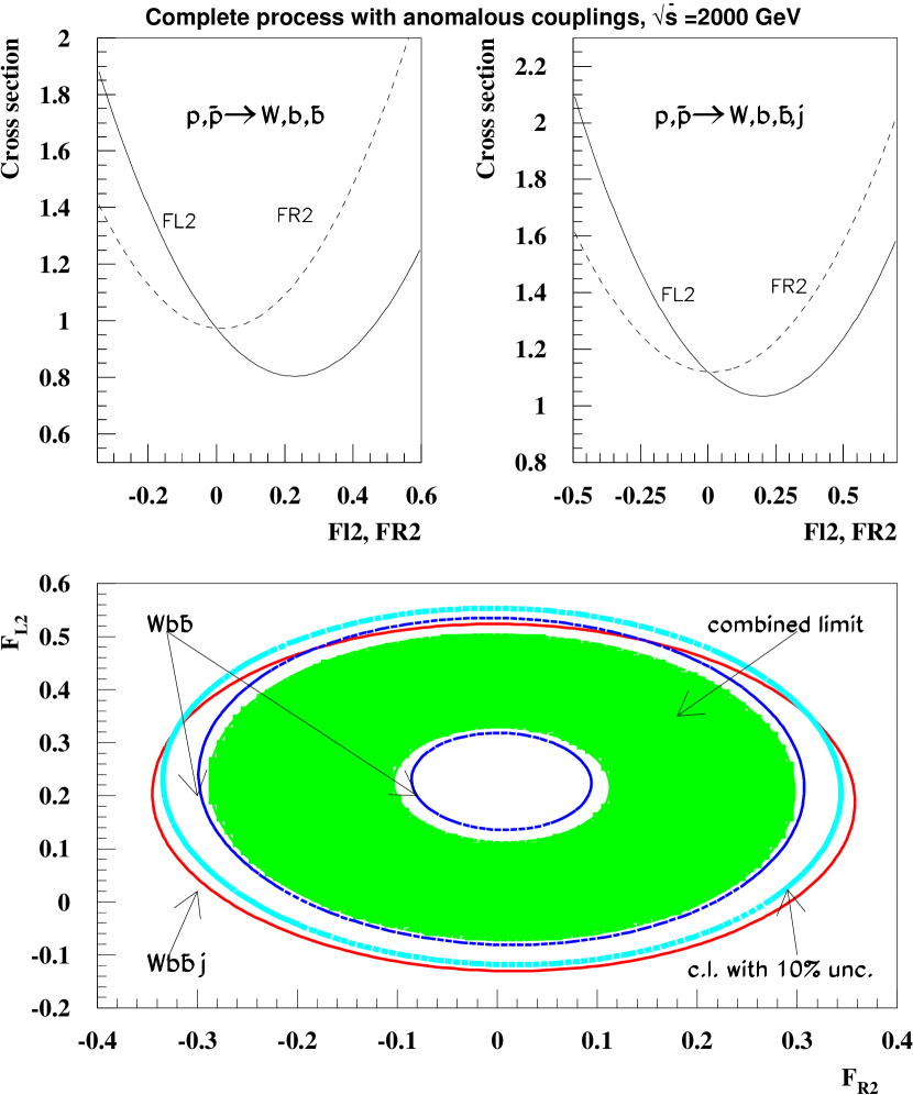
Figure 7: Cross sections after optimized cuts (5a,5c) and corresponding limits on anomalous couplings at the Tevatron.

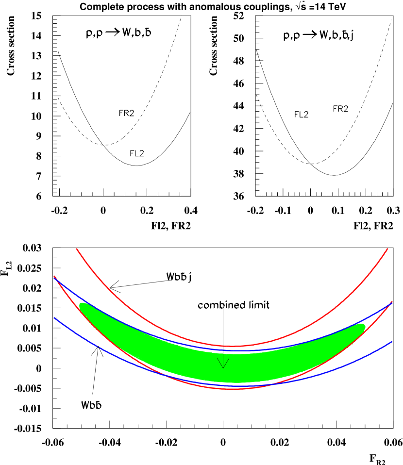
Figure 8: Cross sections after optimized cuts (5b,5d) and corresponding limits on anomalous couplings at the LHC.

The dependence of the total cross section for the processes (1) on anomalous couplings after optimized cuts (5) is shown in the upper part of figure 7 for the Tevatron and in figure 8 for the LHC. The resulting two standard deviation exclusion contours are presented in the lower part of these figures. These exclusion contours correspond to the electronic and muonic decay modes of the $W$-boson, including $\tau$ cascade decays. The combined selection efficiency in the hard kinematical region under consideration, including the double $b$-tagging, is assumed to be $50\%$ and as integrated luminosities we have used $2\text{fb}^{-1}$ for the upgraded Tevatron and $100\text{fb}^{-1}$ for the LHC.

The combined annulus in figure 7 corresponds to the optimistic scenario when only statistical errors are taken into account. A systematic uncertainty of about $10\%$ is expected for the upgraded Tevatron (cf. the last paper in [6]). The resulting exclusion contour is shown in figure 7 as well (the allowed region now covers the hole of the annulus).

Figure 8 demonstrates that it will be essential to measure both processes (1) at the LHC. The allowed regions for the each process alone are rather large annuli, but the overlapping region is much smaller and allows an improvement of the sensitivity on anomalous couplings by an order of magnitude from the Tevatron to the LHC.

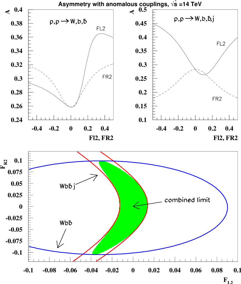
Figure 9: Top-anti-top asymmetry after optimized cuts (5b,5d) and corresponding limits on anomalous couplings at the LHC. (Note that the axes are exchanged with respect to figures 7 and 8.)

The rate of single top production at LHC is different from the rate of single anti-top production. This asymmetry provides an additional observable at LHC that is not available at the Tevatron. The dependence of the asymmetry after optimized cuts (5b,5d) on anomalous couplings and the resulting two standard deviation exclusion contours are shown in figure 9. While the allowed region for the process (1a) is different from the region derived from the rate, the combined limits from both processes (1) are similar.

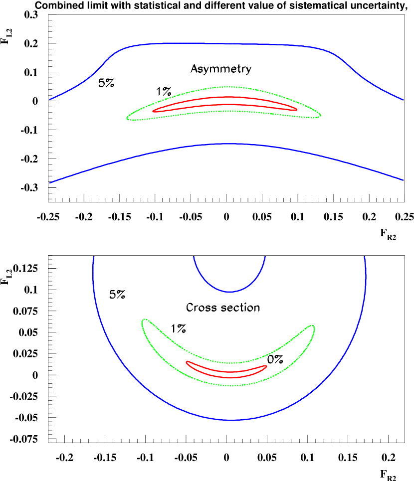
Figure 10: Dependence of the limits on anomalous couplings from LHC measurements on the size of systematical uncertainties.

Systematics			$F_{2}^{L}$			$F_{2}^{R}$
	$\pm$	$10\%$	$-0.18$	$\ldots$	$+0.55$	$-0.24$	$\ldots$	$+0.25$
	$\pm$	$0\%$	$-0.07$	$\ldots$	$+0.11$	$-0.18$	$\ldots$	$+0.21$

Table 2: Uncorrelated limits on anomalous couplings from Tevatron measurements with and without systematical uncertainties.

Systematics			$F_{2}^{L}$			$F_{2}^{R}$
	$\pm$	$10\%$	$-0.094$	$\ldots$	$+0.34$	$-0.17$	$\ldots$	$+0.18$
	$\pm$	$5\%$	$-0.052$	$\ldots$	$+0.097$	$-0.12$	$\ldots$	$+0.13$
	$\pm$	$1\%$	$-0.013$	$\ldots$	$+0.014$	$-0.05$	$\ldots$	$+0.06$
	$\pm$	$0\%$	$-0.003$	$\ldots$	$+0.003$	$-0.022$	$\ldots$	$+0.03$

Table 3: Uncorrelated limits on anomalous couplings from LHC measurements with for several estimates of systematical uncertainties.

Systematical uncertainties (from $\Delta M_{W}$, $\Delta M_{t}$, parton distribution functions, QCD scales, out of cone corrections, luminosity determination, etc.) will play an important role at the LHC as well. It is however impossible to predict them accurately before cross checks from independent measurements at the LHC scale can be performed. Therefore we simply take a set of combined systematic uncertainty and include it into a new fit for each value. Figure 10 shows how the exclusion contours deteriorate when systematic errors of $1\%$ and $5\%$ are included. In the tables 2 and 3, for Tevatron and LHC respectively, the uncorrelated bounds on the anomalous coupling parameters $F_{2}^{L}$ and $F_{2}^{R}$ are given, assuming different systematic uncertainties. Unfortunately, including a $10\%$ systematic error at the LHC will diminish the sensitivity significantly and the allowed regions will be comparable to those obtained at Tevatron.

	$F_{2}^{L}$			$F_{2}^{R}$
Tevatron ($\Delta_{\text{sys.}}\approx 10\%$)	$-0.18$	$\ldots$	$+0.55$	$-0.24$	$\ldots$	$+0.25$
LHC ($\Delta_{\text{sys.}}\approx 5\%$)	$-0.052$	$\ldots$	$+0.097$	$-0.12$	$\ldots$	$+0.13$
$\gamma e$ ($\sqrt{s_{e^{+}e^{-}}}=0.5\text{TeV}$)	$-0.1$	$\ldots$	$+0.1$	$-0.1$	$\ldots$	$+0.1$
$\gamma e$ ($\sqrt{s_{e^{+}e^{-}}}=2.0\text{TeV}$)	$-0.008$	$\ldots$	$+0.035$	$-0.016$	$\ldots$	$+0.016$

Table 4: Uncorrelated limits on anomalous couplings from measurements at different machines.

The potential of the hadron colliders should be compared to the potential a next generation $e^{+}e^{-}$ linear collider (LC) where the best sensitivity could be obtained in high energy $\gamma e$-collisions [4, 5]. The results of this comparison are shown in the Table 4. One can see that a $500\text{GeV}$ LC will outperform the Tevatron (assuming a systematic uncertainty of $10\%$) by a factor of two to five. Nevertheless, the upgraded Tevatron is expected start with physics runs long before a LC. The upgraded Tevatron will therefore be able to perform the first direct measurements of the structure of the $Wtb$ coupling.

The LHC will only be able to rival a $500\text{GeV}$ LC, when the systematic uncertainties can be kept very small (on the order of $1\%$). This goal will be very difficult to achieve. In the more realistic scenario of $5\%$ systematic uncertainties, the LHC will improve the Tevatron limits considerably, but it will fall short of a high energy LC by a factor of three to eight, depending on the coupling under consideration.

In the present analysis, we have not included sources of reducible background [9, 10] to single top production at hadron colliders. However, this reducible background is sufficiently suppressed in the kinematical regions corresponding to our optimized cuts. More detailed simulations and the actual analysis should nevertheless include the tails of these background distributions as well.

Finally, we mention that the exclusion contours in figures 7 and 10 can can be combined with constraints [17, 5] on the right-handed coupling $-0.0015<F^{R}_{2}<0$ from the CLEO measurement of $b\to s\gamma$ [21] to improve the limit on the left-handed coupling $F_{2}^{L}$.

6 Conclusions

We have presented the results of a complete tree level calculation of the processes $pp(\bar{p})\to Wb\bar{b}$ and $Wb\bar{b}+\text{jet}$, taking into account the contributions of anomalous $Wtb$ operators. These final states simultaneously include the single top signal with subsequent decays and irreducible Standard Model backgrounds. We have determined the most sensitive variables from an analysis of the singularities of the Feynman diagrams in phase space, in order to achieve optimal background suppression without sacrificing too much of the signal.

It was shown that the optimized cuts allow to suppress the background rate drastically and to extract limits on anomalous coupling parameters. The accuracy at the LHC is expected to be better by a factor of two to three compared to the upgraded Tevatron. Nevertheless, the Tevatron measurements will provide the first direct information on the structure of the $Wtb$ coupling. For the higher accuracy at LHC, it is essential to measure the two final states separately, to perform efficient double $b$-tagging at high $P^{t}$ and to control the systematic uncertainties at a leverl betetr than $10\%$.

At the LHC, one can reduce the dependence of the results on parton distribution functions, QCD scales, etc. by using the asymmetry of single top and single anti-top production. remains significant after all cuts. Reducible backgrounds are expected to be less important in the phase space region corresponding to the optimized cuts [9, 10]. Nevertheless, a complete simulation including reducible backgrounds and realistic detector response will be required for the final experimental analysis.

Acknowledgments

We acknowledge discussions with A. Pukhov, J. Womersley and B.-L. Young. The work has been supported in part by the grant No. 96-02-19773a of the Russian Foundation of Basic Research, by the Russian Ministry of Science and Technologies, and by the Sankt-Petersburg Grant Center. E. B. and L. D. would like to thank the D0 collaboration and E. B. is also grateful to the CMS collaboration for the kind hospitality during visits at FNAL and CERN. T. O. acknowledges financial support from Bundesministerium für Bildung, Wissenschaft, Forschung und Technologie, Germany.

References

- [1] F. Abe et al., (CDF Collaboration), Phys. Rev. Lett. D74, 2626 (1995); S. Abachi et al., (D0 Collaboration), Phys. Rev. Lett. D74, 2632 (1995); P. Grannis, plenary talk at the International Conference on High Energy Physics, Warsaw, 1996.
- [2] A. Blondel, plenary talk at the International Conference on High Energy Physics, Warsaw, 1996, CERN Report No. LEPEWWG/96-02.
- [3] R. D. Peccei and X. Zhang, Nucl. Phys. B337, 269 (1990); R. D. Peccei, S. Peris, and X. Zhang, Nucl. Phys. B349, 305 (1991).
- [4] E. Boos, A. Pukhov, M. Sachwitz, and H. J. Schreiber, Z. Phys. C75, 237 (1997); Phys. Lett. B404, 119 (1997).
- [5] J.-J. Cao, J.-X. Wang, J.-M. Yang, B.-L. Young, and X. Zhang, Phys. Rev. D58 094004 (1998).
- [6] D. Dicus and S. Willenbrock, Phys. Rev. D34, 155 (1986); C.-P. Yuan, Phys. Rev. D41, 42 (1990); G. V. Jikia and S. R. Slabospitsky, Phys. Lett. B295, 136 (1992); R. K. Ellis and S. Parke, Phys. Rev. D46, 3785 (1992); G. Bordes and B. van Eijk, Z. Phys. C57, 81 (1993); D. O. Carlson and C.-P. Yuan, Phys. Lett. B306, 386 (1993); G. Bordes and B. van Eijk, Nucl. Phys. B435, 23 (1995); S. Cortese and R. Petronzio, Phys. Lett. B253, 494 (1991); D.O. Carlson, E. Malkawi, and C.-P. Yuan, Phys. Lett. B337, 145 (1994); T. Stelzer and S. Willenbrock, Phys. Lett. B357, 125 (1995); R. Pittau, Phys. Lett. B386, 397 (1996); M. Smith and S. Willenbrock, Phys. Rev. D54, 6696 (1996); D. Atwood, S. Bar-Shalom, G. Eilam, and A. Soni, Phys. Rev. D54, 5412 (1996); C. S. Li, R. J. Oakes, and J. M. Yang, Phys. Rev. D55, 1672 (1997); C. S. Li, R. J. Oakes, and J. M. Yang, Phys. Rev. D55, 5780 (1997); G. Mahlon, S. Parke, Phys. Rev. D55, 7249 (1997); A. P. Heinson, A. S. Belyaev, and E. E. Boos, Phys. Rev. D56, 3114 (1997); T. Stelzer, Z. Sullivan, and S. Willenbrock, Phys. Rev. D56, 5919 (1997); T. Tait and C.-P. Yuan, MSUHEP-71015, hep-ph/9710372; D. Atwood, S. Bar-Shalom, G. Eilam, and A. Soni, Phys. Rev. D57, 2957 (1998); T. Stelzer, Z. Sullivan, and S. Willenbrock, Phys. Rev. D58 094021 (1998); A. Belyaev, E. Boos, and L. Dudko, Phys. Rev. D59, 075001 (1999), hep-ph/9806332.
- [7] M. Smith and S. Willenbrock, Phys. Rev. D54, 6696 (1996); T. Stelzer, Z. Sullivan, and S. Willenbrock, Phys. Rev. D56, 5919 (1997).
- [8] A. P. Heinson, A. S. Belyaev, E. E. Boos, Phys. Rev. D56, 3114 (1997).
- [9] A. Belyaev, E. Boos, and L. Dudko, Phys. Rev. D59, 075001 (1999), hep-ph/9806332.
- [10] T. Stelzer, Z. Sullivan, and S. Willenbrock, Phys. Rev. D58 09402 (1998).
- [11] N. V. Dokholyan and G. V. Jikia, Phys. Lett. B336, 251 (1994); E. E. Boos et al., Z. Phys. C70, 255 (1996).
- [12] A. Stange, W. Marciano, and S. Willenbrock, Phys. Rev. D50, 4491 (1994); A. Belyaev, E. E. Boos, and L. Dudko, Mod. Phys. Lett. A10, 25 (1995).
- [13] E. E. Boos, M. N. Dubinin, V. A. Ilyin, A. E. Pukhov, and V.I. Savrin, INP MSU 94-36/358 and SNUTP-94-116, hep-ph/9503280; P. Baikov et al., in Proc. of the Xth Int. Workshop on High Energy Physics and Quantum Field Theory, QFTHEP-95, ed. by B. Levtchenko and V. Savrin, (Moscow, 1995), p. 101.
- [14] V. A. Ilyin, D. N. Kovalenko, and A. E. Pukhov, Int. J. Mod. Phys. C7, 761 (1996); D. N. Kovalenko and A. E. Pukhov, Nucl. Instrum. and Meth. A389, 299 (1997).
- [15] H. Lai, J. Huston, S. Kuhlmann, F. Olness, J. Owens, D. Soper, W.-K. Tung, and H. Weerts (CTEQ Collaboration), Phys. Rev. D55, 1280 (1997).
- [16] W. Buchmüller and D. Wyler, Nucl. Phys. B268, 621 (1986); K. Hagiwara, S. Ishihara, R. Szalarski, and D. Zeppenfeld, Phys. Rev. D48, 2182 (1993); K. Hagiwara, R. Szalarski, and D. Zeppenfeld, Phys. Lett. B318, 155 (1993); B. Grzadkowski and J. Wudka, Phys. Lett. B364, 49 (1995); G. J. Gounaris, F. M. Renard, and N. D. Vlachos, Nucl. Phys. B459, 51 (1996).
- [17] K. Whisnant, J. M. Yang, B.-L. Young, and X. Zhang, Phys. Rev. D56, 467 (1997).
- [18] G. L. Kane, G. A. Ladinsky, and C.-P. Yuan, Phys. Rev. D45, 124 (1992).
- [19] E. Boos and L. Dudko, in preparation.
- [20] C. Caso et al., Particle Data Group, Eur. Phys. J. C3, 1 (1998).
- [21] M. Alam et al., CLEO Collaboration, Phys. Rev. Lett. 74, 2885 (1995).