BUTP–99/03 hep-ph/9902480
TTP99–10 February 1999
Non-Singlet Corrections of ${\cal O}(\alpha_{s}^{2}G_{F}M_{t}^{2})$ to $\Gamma(Z\to b\bar{b})$

Abstract

The partial decay rate of the $Z$ boson into bottom quarks constitutes an important decay channel. This is mainly due to the virtual presence of the top quark in the loop diagrams giving rise to correction factors which are quadratic in the top quark mass. At one- and two-loop order it turned out that the leading term in the heavy-top expansion leads to very good approximations to the exact result. In this work the non-singlet diagrams at ${\cal O}(\alpha_{s}^{2}G_{F}M_{t}^{2})$ are considered.

The impressive experimental precision mainly at the Large Electron Positron collider (LEP) at CERN, the Stanford Linear Collider (SLC) and the FERMILAB Tevatron in Chicago has made it mandatory to evaluate higher order quantum corrections to the processes observed in the experiments [1]. The strategy to combine experimental information with theoretical computations has successfully been applied to the search for the top quark several years ago. Nowadays the same concept is used in order to pin down the mass of the Higgs boson, the only not yet discovered particle of the Standard Model of elementary particle physics.

An important observable is the decay of the $Z$ boson into bottom. QCD corrections are known up to ${\cal O}(\alpha_{s}^{3})$ (for a comprehensive review see [2]). The electroweak one-loop corrections are known since quite some time [3]. They have the interesting feature that the top quark appears virtually in the loop diagrams. Recently also the full corrections of ${\cal O}(\alpha\alpha_{s})$ were completed [4, 5, 6]. The diagrams involving a top quark are considered in [6] where the first five terms in the expansion for a heavy top quark mass, $M_{t}$, is computed. It was demonstrated that these terms approximate the exact result quite well. Actually it turned out that both at ${\cal O}(\alpha)$ and ${\cal O}(\alpha\alpha_{s})$ a large cancellation between the sub-leading terms takes place and effectively only the leading term proportional to $G_{F}M_{t}^{2}$ [7] remains. This is a strong motivation to look at the next order in the strong coupling constant and evaluate the leading terms. To the corrections enhanced by the top quark mass only those contributions have to be considered where a scalar particle, namely the Higgs boson, $H$, the neutral Goldstone boson, $\chi$, or the charged one, $\phi^{\pm}$, couples to the top quark. Thus no diagrams have to be considered where the $W$ or $Z$ boson appear as internal lines.

Corrections of this order were first computed for the $\rho$ parameter [8], the ratio of the charged and neutral current amplitude, where it turned out that they are quite important [9]. Later on also the hadronic Higgs decay was analyzed at ${\cal O}(\alpha_{s}^{2}G_{F}M_{t}^{2})$ [10, 11]. In the case of the Higgs boson one can exploit that the scalar coupling is proportional to the mass which simplifies the construction of an effective Lagrangian and especially the subsequent evaluation of the diagrams. Actually the whole computation could be reduced to the evaluation of two-point functions. We will see below that in the case of the $Z$ boson one should also consider vertex diagrams.

It has become customary to parametrize the corrections proportional to $M_{t}^{2}$ by the quatity

$$X_{t} = \frac{G_{F}M_{t}^{2}}{8\pi^{2}\sqrt{2}}\,,$$ (1)

respectively the quantity $x_{t}$ which is defined using the ${\overline{\rm MS}}$ definition of the top quark mass, $m_{t}$.

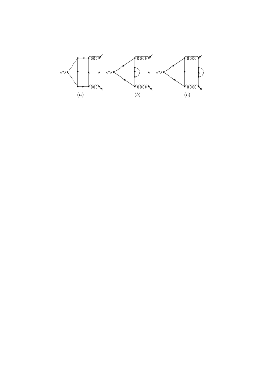
Figure 1: Singlet diagrams contributing at ${\cal O}(\alpha_{s}^{2}X_{t})$ to the hadronic $Z$ boson decay. In $(a)$ and $(c)$ the dashed line correspond to the charged Goldstone boson whereas in $(b)$ it may also be the Higgs or the neutral Goldstone boson. Diagrams $(a)$ and $(b)$ are of universal type whereas $(c)$ constitutes a non-universal contribution to $\Gamma(Z\to b\bar{b})$. In the displayed examples the thick lines correspond to top quarks whereas the thin lines represent bottom quarks.

The quantum corrections to $\Gamma(Z\to b\bar{b})$ are divided into universal ones which are identical for all quark species and non-universal parts which are specific for the $Zb\bar{b}$ vertex. Both the universal and non-universal corrections are divided into singlet and non-singlet parts. The singlet contributions arise from those diagrams where the $Z$ boson and the bottom quarks of the final state couple to different fermion lines. Another class of singlet contributions is constituted by the diagrams where the $Z$ boson couples to two charged Goldstone bosons which in turn form together with two gluons a box diagram and the gluons finally couple to the quarks in the final state. In Fig. 1 some sample diagrams are listed. Fig. 1$(a)$ and $(b)$ are of universal nature whereas in $(c)$ the Goldstone boson in directly coupled to the final state bottom quark thus providing a non-universal contribution. In this article only non-singlet diagrams will be computed; the singlet contributions will be considered elsewhere. The universal corrections of ${\cal O}(\alpha_{s}^{2}X_{t})$ are in part governed by the $\rho$ parameter [9]. A second source for universal corrections arise from those diagrams where only gluons couple to the light quark lines. The gluons split into a fermion loop actually formed by bottom and top quarks accompanied by an additional exchange of a scalar particle (cf. Fig. 2$(a)$). The main focus of this paper is devoted to the evaluation of the non-universal non-singlet diagrams. Typical examples are pictured in Fig. 2$(b)$-$(e)$.

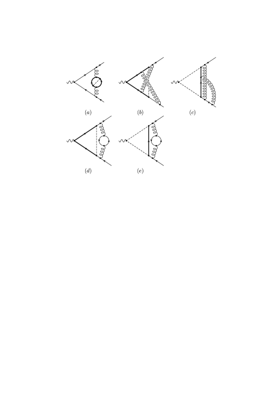
Figure 2: Non-singlet contributions of ${\cal O}(\alpha_{s}^{2}X_{t})$ to the hadronic $Z$ boson decay. In $(a)$ the dashed line corresponds to the Higgs boson or the neutral or charged Goldstone boson. In the diagrams $(b)-(e)$ only the charged Goldstone boson is allowed. Diagram $(a)$ is of universal type whereas $(b)-(e)$ constitute non-universal contributions to $\Gamma(Z\to b\bar{b})$. In the displayed examples the thick lines correspond to top quarks whereas the thin lines represent bottom quarks.

In a first step an effective Lagrangian is constructed were the top quark is integrated out. Thereby it is convenient to split the fermion fields into their left and right part and consider them separately. It is furthermore necessary to decouple the bottom quark fields using the relations (see e.g. [10]):

$$b_{L/R}^{0\prime} = \sqrt{\zeta_{2,b}^{0,L/R}}b_{L/R}^{0}\,,$$ (2)

where the primes denote the quantities in the effective theory and the superscript “0” reminds that we are still dealing with bare quantities. The decoupling constants $\zeta_{2,b}^{0,L/R}$ can be computed with the help of

$$\zeta_{2,b}^{0,L/R} = 1+\Sigma_{b,V}^{0h}\mp\Sigma_{b,A}^{0h}\,,$$ (3)

where $\Sigma_{b,V}^{0h}$ and $\Sigma_{b,A}^{0h}$ is the vector and axial-vector part of the bottom quark self energy. Here only the hard part, i.e. those diagrams containing the top quark, has to be computed which is indicated by the index “h”. Finally the part of the effective Lagrangian describing the interaction of the $Z$ boson to bottom quarks has the form

$${\cal L}_{\rm eff} \sim \left[C_{L}^{0}\bar{b}_{L}^{0\prime}\gamma^{\mu}b_{L}^{0\prime}+C_{R}^{0}\bar{b}_{R}^{0\prime}\gamma^{\mu}b_{R}^{0\prime}\right]Z_{\mu}\,.$$ (4)

The residual dependence on $M_{t}$ is contained in the coefficient functions $C_{L/R}^{0}$. They are obtained from the hard part of the $Zb\bar{b}$ vertex:

$$C_{L/R}^{0} = \frac{\Gamma_{Zb\bar{b}}^{h,L/R}}{\zeta_{2,b}^{0,L/R}}\,.$$ (5)

Here, the left and right part of the $Zb\bar{b}$ vertex are defined through:

$$\Gamma_{Zb\bar{b},\mu}^{h}\,\,=\,\,\gamma_{\mu}\left[\Gamma_{Zb\bar{b}}^{h,V}+\gamma_{5}\Gamma_{Zb\bar{b}}^{h,A}\right]\,, \Gamma_{Zb\bar{b}}^{h,L/R}\,\,=\,\,\Gamma_{Zb\bar{b}}^{h,V}\mp\Gamma_{Zb\bar{b}}^{h,A}\,,$$ (6)

where it is understood that in addition to the top-induced diagrams also the tree-level terms are included. The coefficient functions of Eq. (5) are finite after the coupling constant $\alpha_{s}$ and the mass of the top quark are expressed through their renormalized counterparts. This is because the vector and axial-vector currents have vanishing anomalous dimension as long as only non-singlet diagrams are considered. Thus from now on the index “0” is omitted.

In order to evaluate the partial decay rate of the $Z$ boson into bottom quarks at ${\cal O}(\alpha_{s}^{2}X_{t})$ one has to evaluate the coefficient functions up to this accuracy. Furthermore the pure QCD corrections in the effective theory are needed up to order $\alpha_{s}^{2}$. It can be taken over from [12] and reads:

$$\delta^{(5),QCD} = 1+\frac{\alpha_{s}^{(5)}(\mu)}{\pi}+\left(\frac{\alpha_{s}^{(5)}(\mu)}{\pi}\right)^{2}\bigg{[}\frac{365}{24}-11\,\zeta_{3}$$ (7)

$$\mbox{}+n_{l}\left(-\frac{11}{12}+\frac{2}{3}\,\zeta_{3}\right)+\left(-\frac{11}{4}+\frac{1}{6}n_{l}\right)\ln\frac{M_{Z}^{2}}{\mu^{2}}\bigg{]}\,,$$

where $n_{l}=5$ is the number of light quarks and $\zeta_{i}$ is Riemann’s Zeta function with the value $\zeta_{3}\approx 1.202056903$.

The computation of the decoupling constants for the bottom quark field up to order $\alpha_{s}^{2}X_{t}$ has been performed in [10]. The only missing pieces are the vector and axial-vector contributions to the hard part of the $Zb\bar{b}$ vertex. Some sample diagrams are listed in Fig. 2. As mentioned above only those diagrams have to be taken into account which contain a virtual top quark. Note that for the very calculation it is possible to nullify all external momenta. At one-loop order only two diagrams have to be considered. This increases to $19$ at the two-loop level which is still feasible by hand. In the order we are interested in, however, more than 350 diagrams have to be considered, which makes the extensive use of computer algebra necessary. For the present calculation the package GEFICOM [13] has been used. It passes the generation of the diagrams to QGRAF [14] and uses for the very computation of the integrals the program MATAD [15] which is written in FORM [16] for the purpose to compute one-, two- and three-loop vacuum graphs. For a recent review concerned with the automatic computation of Feynman diagrams see [17].

Expressed in terms of the ${\overline{\rm MS}}$ top quark mass the result for the coefficient functions read:

$$C_{L} = \frac{e}{s_{\theta}c_{\theta}}\Bigg{\{}-\frac{1}{2}+\frac{1}{3}s_{\theta}^{2}+x_{t}\Bigg{[}1+\frac{\alpha_{s}^{(6)}(\mu)}{\pi}\,C_{F}\,\left(2-\frac{3}{2}\zeta_{2}+\frac{3}{2}\ln\frac{\mu^{2}}{m_{t}^{2}}\right)$$ (8)

$$\mbox{}+\left(\frac{\alpha_{s}^{(6)}(\mu)}{\pi}\right)^{2}\Bigg{(}C_{F}^{2}\bigg{(}-\frac{49}{192}-\frac{199}{48}\zeta_{2}+\frac{253}{12}\zeta_{3}-\frac{77}{8}\zeta_{4}+\frac{5}{4}B_{4}-\frac{5}{8}D_{3}-\frac{1053}{32}S_{2}$$

$$\mbox{}+\left(\frac{15}{16}-\frac{9}{4}\zeta_{2}\right)\ln\frac{\mu^{2}}{m_{t}^{2}}+\frac{9}{8}\ln^{2}\frac{\mu^{2}}{m_{t}^{2}}\bigg{)}+C_{A}C_{F}\bigg{(}\frac{461}{64}-\frac{99}{32}\zeta_{2}-\frac{187}{24}\zeta_{3}+\frac{61}{16}\zeta_{4}$$

$$\mbox{}-\frac{5}{8}B_{4}+\frac{5}{16}D_{3}+\frac{1053}{64}S_{2}+\left(\frac{185}{48}-\frac{11}{8}\zeta_{2}\right)\ln\frac{\mu^{2}}{m_{t}^{2}}+\frac{11}{16}\ln^{2}\frac{\mu^{2}}{m_{t}^{2}}\bigg{)}$$

$$\mbox{}+C_{F}Tn_{l}\bigg{(}-\frac{95}{48}+\frac{4}{3}\zeta_{2}-\zeta_{3}+\left(-\frac{13}{12}+\frac{1}{2}\zeta_{2}\right)\ln\frac{\mu^{2}}{m_{t}^{2}}-\frac{1}{4}\ln^{2}\frac{\mu^{2}}{m_{t}^{2}}\bigg{)}$$

$$\mbox{}+C_{F}T\bigg{(}\frac{149}{240}-\frac{1}{60}\zeta_{2}-\frac{35}{8}\zeta_{3}+\frac{729}{40}S_{2}+\left(-\frac{13}{12}+\frac{1}{2}\zeta_{2}\right)\ln\frac{\mu^{2}}{m_{t}^{2}}-\frac{1}{4}\ln^{2}\frac{\mu^{2}}{m_{t}^{2}}\bigg{)}\Bigg{)}\Bigg{]}\Bigg{\}}$$

$$= \mbox{}\frac{e}{s_{\theta}c_{\theta}}\Bigg{\{}-\frac{1}{2}+\frac{1}{3}s_{\theta}^{2}+x_{t}\Bigg{[}1+\frac{\alpha_{s}^{(6)}(\mu)}{\pi}\left(\frac{8}{3}-2\zeta_{2}+2\ln\frac{\mu^{2}}{m_{t}^{2}}\right)$$

$$\mbox{}+\left(\frac{\alpha_{s}^{(6)}(\mu)}{\pi}\right)^{2}\Bigg{(}\frac{62149}{2160}-\frac{21337}{1080}\zeta_{2}+\frac{367}{108}\zeta_{3}-\frac{67}{36}\zeta_{4}-\frac{5}{18}B_{4}+\frac{5}{36}D_{3}+\frac{1557}{80}S_{2}$$

$$\mbox{}+n_{l}\left(-\frac{95}{72}+\frac{8}{9}\zeta_{2}-\frac{2}{3}\zeta_{3}\right)+\left(\frac{589}{36}-\frac{55}{6}\zeta_{2}+n_{l}\left(-\frac{13}{18}+\frac{1}{3}\zeta_{2}\right)\right)\ln\frac{\mu^{2}}{m_{t}^{2}}$$

$$\mbox{}+\left(\frac{55}{12}-\frac{1}{6}n_{l}\right)\ln^{2}\frac{\mu^{2}}{m_{t}^{2}}\Bigg{)}\Bigg{]}\Bigg{\}}\,,$$

$$C_{R} = \frac{e}{s_{\theta}c_{\theta}}\frac{1}{3}s_{\theta}^{2}\,,$$

with $m_{t}=m_{t}(\mu)$. After the second equal sign the colour factors $C_{F}=4/3,C_{A}=3$ and $T=1/2$ have been inserted. $\zeta_{2}=\pi^{2}/6$ and $\zeta_{4}=\pi^{4}/90$. $s_{\theta}$ and $c_{\theta}$ are the sine and cosine of the weak mixing angle. The constants $B_{4}$, $D_{3}$ and $S_{2}$ typically appear in the result of three-loop vacuum integrals and read [18, 9, 19]:

$$S_{2} = {4\over 9\sqrt{3}}\mbox{Cl}_{2}\left({\pi\over 3}\right)\,\,\approx\,\,0.260\,434\,,$$

$$D_{3} = 6\zeta_{3}-\frac{15}{4}\zeta_{4}-6\left(\mbox{Cl}_{2}\left({\pi\over 3}\right)\right)^{2}\,\,\approx\,\,-3.027\,009\,,$$

$$B_{4} = 16\mbox{Li}_{4}\left({1\over 2}\right)-{13\over 2}\zeta_{4}-4\zeta_{2}\ln^{2}2+{2\over 3}\ln^{4}2\,\,\approx\,\,-1.762\,800\,.$$ (9)

Note that according to the QED Ward identity the universal corrections induced by the diagrams in Fig. 2$(a)$ cancel in the coefficient functions against the corresponding part in the quark self energy. As we consider in addition the bottom quark to be massless the right-handed coefficient function sticks to its Born value. Using the relation between $m_{t}$ and the on-shell mass $M_{t}$ [20] one gets:

$$C_{L}^{OS} = \frac{e}{s_{\theta}c_{\theta}}\Bigg{\{}-\frac{1}{2}+\frac{1}{3}s_{\theta}^{2}+X_{t}\Bigg{[}1-2\zeta_{2}\frac{\alpha_{s}^{(6)}(\mu)}{\pi}+\left(\frac{\alpha_{s}^{(6)}(\mu)}{\pi}\right)^{2}\Bigg{(}\frac{1054}{135}-\frac{19897}{1080}\zeta_{2}+\frac{403}{108}\zeta_{3}$$ (10)

$$\mbox{}-\frac{67}{36}\zeta_{4}-\frac{4}{3}\zeta_{2}\ln 2-\frac{5}{18}B_{4}+\frac{5}{36}D_{3}+\frac{1557}{80}S_{2}+n_{l}\left(-\frac{1}{3}+\frac{14}{9}\zeta_{2}-\frac{2}{3}\zeta_{3}\right)$$

$$\mbox{}+\left(-\frac{31}{6}+\frac{1}{3}n_{l}\right)\zeta_{2}\ln\frac{\mu^{2}}{M_{t}^{2}}\Bigg{)}\Bigg{]}\Bigg{\}}\,,$$

$$C_{R}^{OS} = C_{R}\,.$$

Let us now turn to a brief numerical discussion of the new results. The decay rate can be computed with the help of

$$\Gamma(Z\to b\bar{b}) = \frac{N_{C}M_{Z}}{24\pi}\left(C_{L}^{2}+C_{R}^{2}\right)\,\delta^{(5),QCD}\,.$$ (11)

Actually two scales are involved in the process, namely $M_{Z}$ and the mass of the top quark. The resummation of potentially large logarithms is, however, trivial as both $C_{L/R}$ and $\delta^{(5),QCD}$ are separately renormalization group invariant. Thus the scale parameter $\mu$ may be set to $m_{t}$, respectively, $M_{t}$ in the coefficient functions and to $M_{Z}$ in the massless corrections. For these choices the numerical expansions of the ingredients for Eq. (11) read:

$$\delta^{(5),QCD} = 1+\frac{\alpha_{s}^{(5)}(M_{Z})}{\pi}+1.409\left(\frac{\alpha_{s}^{(5)}(M_{Z})}{\pi}\right)^{2}\,,$$

$$C_{L} = \frac{e}{s_{\theta}c_{\theta}}\Bigg{\{}-\frac{1}{2}+\frac{1}{3}s_{\theta}^{2}+x_{t}\Bigg{[}1-0.623\frac{\alpha_{s}^{(6)}(\mu_{t})}{\pi}+0.190\left(\frac{\alpha_{s}^{(6)}(\mu_{t})}{\pi}\right)^{2}\Bigg{]}\Bigg{\}}\,,$$

$$C_{L}^{OS} = \frac{e}{s_{\theta}c_{\theta}}\Bigg{\{}-\frac{1}{2}+\frac{1}{3}s_{\theta}^{2}+X_{t}\Bigg{[}1-3.290\frac{\alpha_{s}^{(6)}(M_{t})}{\pi}-9.288\left(\frac{\alpha_{s}^{(6)}(M_{t})}{\pi}\right)^{2}\Bigg{]}\Bigg{\}}\,,$$ (12)

with $\mu_{t}=m_{t}(m_{t})$. $n_{l}=5$ has been chosen.

Concerning the enhanced corrections of ${\cal O}(X_{t})$ to the coefficient functions the same observations can be made as for the $\rho$ parameter [9] and the various quantities in connection with the Higgs decay [21, 10]: Expressed in terms of the on-shell top quark mass the leading order term is “screened” by the QCD corrections as they enter with a different sign. On the other hand, the coefficients turn out to be much smaller in the ${\overline{\rm MS}}$ scheme. Actually the coefficient in front of the three-loop term is smaller by a factor of 50 as compared to the corresponding one in the on-shell scheme. Furthermore the sign is alternating which also indicates a faster convergence if the ${\overline{\rm MS}}$ mass is used for the parameterization.

Inserting Eqs. (12) into Eq. (11) finally leads to the following $M_{t}^{2}$-enhanced terms:

$$\Gamma^{x_{t}}(Z\to b\bar{b}) = \frac{N_{C}M_{Z}\alpha}{6s_{\theta}^{2}c_{\theta}^{2}}\left(-1+\frac{2}{3}s_{\theta}^{2}\right)x_{t}\left[1+0.0161+0.0014\right]\,,$$ (13)

$$\Gamma^{X_{t}}_{OS}(Z\to b\bar{b}) = \frac{N_{C}M_{Z}\alpha}{6s_{\theta}^{2}c_{\theta}^{2}}\left(-1+\frac{2}{3}s_{\theta}^{2}\right)X_{t}\left[1-0.074-0.0130\right]\,,$$ (14)

where the values $\alpha_{s}^{(5)}(M_{Z})=0.118$, $\alpha_{s}^{(6)}(M_{t})=0.107$ and $\alpha_{s}^{(6)}(m_{t})=0.108$ have been used. The numbers in the squared brackets correspond to the corrections with increasing power in $\alpha_{s}$. The index $OS$ reminds on the definition of the top quark mass used and as before the index ${\overline{\rm MS}}$ is suppressed. In the $\overline{\rm MS}$ scheme the second order QCD corrections amount to roughly 9% of the first order ones, however, the overall size is quite small. The order $\alpha_{s}$ corrections to the leading $X_{t}$ term in the on-shell scheme is almost by a factor of five larger than in the $\overline{\rm MS}$ scheme and the corresponding ${\cal O}(\alpha_{s}^{2})$ corrections amount to almost 18% of the ${\cal O}(\alpha_{s})$ term. It is actually almost as large as the ${\cal O}(\alpha_{s})$ term in Eq. (13).

To summarize, quantum corrections of ${\cal O}(\alpha_{s}^{2}x_{t})$ to the decay of the $Z$ boson into bottom quarks have been computed. If we assume that the observations made at one- and two-loop level are also true at order $\alpha_{s}^{2}X_{t}$ a substantial part of the corrections is available. Expressed in terms of the ${\overline{\rm MS}}$ mass they turn out to be tiny. In the on-shell scheme the quantum corrections are much larger and they screen the leading $X_{t}$ term by almost 9%. Note that the newly computed term of ${\cal O}(\alpha_{s}^{2}x_{t})$ makes it possible to use the combination of the three-loop $\rho$ parameter [9] and the partial width $\Gamma(Z\to b\bar{b})$ in a consistent way.

References

[1]
D. Karlen, talk presented at ICHEP ’98, Vancouver, July 1998;
W. Hollik, talk presented at ICHEP ’98, Vancouver, July 1998;
F. Teubert, Proceedings of the IVth Int. Symp. on
Radiative Corrections, Barcelona, Sept. 8-12, 1998; hep-ph/9811414.
[2]
K.G. Chetyrkin, J.H. Kühn, and A. Kwiatkowski,
Phys. Reports 277 (1996) 189.
[3]
A. Akhundov, D. Bardin, and T. Riemann,
Nucl. Phys.B 276 (1986) 1;
W. Beenakker and W. Hollik, Z. Phys.C 40 (1988) 141;
J. Bernabeu, A. Pich, and A. Santamaria,
Phys. Lett.B 200 (1988) 569;
B.W. Lynn and R.G. Stuart Phys. Lett.B 252 (1990) 676.
[4]
A.L. Kataev, Phys. Lett.B 287 (1992) 209.
[5]
A. Czarnecki and J.H. Kühn, Phys. Rev. Lett.77 (1996) 3955;
(E) ibid.80(1998) 893.
[6]
R. Harlander, T. Seidensticker, and M. Steinhauser,
Phys. Lett.B 426 (1998) 125.
[7]
J. Fleischer, F. Jegerlehner, P. Ra̧czka, and O.V. Tarasov,
Phys. Lett.B 293 (1992) 437;
G. Buchalla and A. Buras, Nucl. Phys.B 398 (1993) 285;
G. Degrassi, Nucl. Phys.B 407 (1993) 271;
K.G. Chetyrkin, A. Kwiatkowski, and M. Steinhauser,
Mod. Phys. Lett.A 8 (1993) 2785.
[8]
M. Veltman, Nucl. Phys.B 123 (1977) 89.
[9]
L. Avdeev, J. Fleischer, S. Mikhailov, and O. Tarasov,
Phys. Lett.B 336 (1994) 560,
(E) ibid.B 349 (1995) 597;
K.G. Chetyrkin, J.H. Kühn, and M. Steinhauser,
Phys. Lett.B 351 (1995) 331;
Phys. Rev. Lett.75 (1995) 3394.
[10]
K.G. Cheyrkin, B.A. Kniehl, and M. Steinhauser,
Nucl. Phys.B 490 (1997) 19;
Phys. Rev. Lett.78 (1997) 594.
[11]
M. Steinhauser, Phys. RevD 59 (1999) 054005.
[12]
K.G. Chetyrkin, A.L. Kataev, and F.V. Tkachov,
Phys. Lett.B 85 (1979) 277;
M. Dine and J. Sapirstein,
Phys. Rev. Lett.43 (1979) 668;
W. Celmaster and R.J. Gonsalves,
Phys. Rev. Lett.44 (1980) 560.
[13]
K.G. Chetyrkin and M. Steinhauser, unpublished.
[14]
P. Nogueira, J. Comp. Phys. 105 (1993) 279.
[15]
M. Steinhauser, Ph.D. thesis, Karlsruhe University
(Shaker Verlag, Aachen, 1996).