YITP-99-5

UT-836

KUNS-1559

TUM-HEP-344/99

SFB-375-333

Anomalous U(1) Gauge Symmetry and
Lepton Flavor Violation

Kiichi Kurosawa and Nobuhiro Maekawa

^aYITP, Kyoto University, Kyoto 606-8502, Japan
^aDepartment of Physics, University of Tokyo,
Tokyo 113-0033, Japan
^bDepartment of Physics, Kyoto University,
Kyoto 606-8502, Japan
^bPhysik Department, Technische Universität München,
D-85748 Garching, Germany

In recent years, many people have studied the possibility that the anomalous $U(1)$ gauge symmetry is a trigger of SUSY breaking and/or an origin of the fermion mass hierarchy. Though it is interesting that the anomalous $U(1)$ symmetry may explain these two phenomena simultaneously, it causes a negative stop mass squared or a severe fine-tuning in order to avoid the FCNC problem. Recently, it was pointed out that the $F$-term contribution of the dilaton field can dominate the flavor-dependent contribution from the anomalous $U(1)$ $D$-term, so that the FCNC problem may be naturally avoided. In this paper, we study the case in which the dilaton is stabilized by the deformation of the Kähler potential for the dilaton and find that the order of the ratio of the $F$-term to the $D$-term contributions is generally determined. This implies that the branching ratio of $\mu\to e\gamma$ can be found around the present experimental bound.

1 Introduction

One of the most important problems of the standard model is the stability of the weak scale and another is the hierarchy problem of fermion masses. The most promising solution for the former problem is to introduce supersymmetry (SUSY). If SUSY is realized in nature, we should understand the origin of SUSY breaking. One of the possibilities is that an anomalous $U(1)$ gauge symmetry with anomaly cancellation due to the Green-Schwarz mechanism [1] triggers SUSY breaking [2, 3] and mediates the SUSY breaking effects in ordinary matter [4]. On the other hand, it is widely known that the latter problem of the fermion mass hierarchy can be solved by assignment of anomalous $U(1)$ charges to the matter fields [5, 6]. It is interesting to examine the possibility that the anomalous $U(1)$ gauge symmetry explains both the origin of SUSY breaking and the origin of fermion mass hierarchy [7, 8]. However, there are some unsettled issues for this scenario. In order to explain the fermion mass hierarchy, we should assign anomalous $U(1)$ charges dependent on the flavor. This induces non-degenerate scalar fermion masses through the anomalous $U(1)$ $D$-term. The large SUSY breaking scale allows us to avoid the flavor changing neutral current (FCNC) problem [9, 10], while it causes a negative stop mass squared or a severe fine-tuning [11].

Recently, Arkani-Hamed, Dine and Martin [12] pointed out that the $F$-term contribution of the dilaton field can be larger than the anomalous $U(1)$ $D$-term contribution, depending on how the dilaton is stabilized. If the $F$-term contribution dominates the $D$-term contribution, the situation is drastically changed. Through loop corrections of the gaugino, the $F$-term contribution can induce degenerate scalar fermion masses. As a result, the constraints from FCNC processes are weakened.

In this paper, we point out that the order of the ratio of the $D$-term to the $F$-term contributions is generally determined when the dilaton is stabilized by smallness of the second derivative of the Kähler potential for the dilaton. The $D$-term gives the flavor-dependent sfermion masses, while the $F$-term of the dilaton contributes the flavor-independent sfermion masses through loop corrections of the gaugino. Therefore FCNC processes can be predicted by this ratio. In this scenario the most dangerous process is the $\mu\to e\gamma$ process, and it can be found around the present experimental bound to the branching ratio $BR(\mu\to e\gamma)<4.9\times 10^{-11}$ [13]. We also investigate the case in which there are other contributions to sfermion masses as well as loop corrections of the gaugino. Even in this case, the branching ratio is not so different from the current bound.

2 Anomalous $U(1)$ gauge symmetry

First we review the anomalous $U(1)_{A}$ gauge symmetry. It is well-known that some low energy effective theories of string theory include the anomalous $U(1)_{A}$ gauge symmetry that has non-zero anomalies, such as the pure $U(1)_{A}^{3}$ anomaly, mixed anomalies with the other gauge groups $G_{a}$, and the mixed gravitational anomaly [14]. These anomalies are canceled by combining the nonlinear transformation of the dilaton chiral supermultiplet $S$ with the gauge transformation of the $U(1)_{A}$ vector supermultiplet $V_{A}$:

$$V_{A} \to V_{A}+\frac{i}{2}\left(\Lambda-\Lambda^{\dagger}\right),$$ (2.1)

$$S \to S+\frac{i}{2}\,\delta_{GS}\,\Lambda,$$ (2.2)

where $\Lambda$ is a parameter chiral superfield. This cancellation occurs because the gauge kinetic functions for $V_{A}$ and the other vector supermultiplets $V_{a}$ are given by

$${\cal L}_{\mbox{\scriptsize gauge}}=\frac{1}{4}\int d^{2}\theta\left[\,k_{A}S\,W_{A}{}^{\alpha}W_{A}{}_{\alpha}+k_{a}S\,W_{a}{}^{\alpha}W_{a}{}_{\alpha}\,\right]+\mbox{h.c.},$$ (2.3)

where $W_{A}{}^{\alpha}$ and $W_{a}{}^{\alpha}$ are the chiral projected superfields from $V_{A}$ and $V_{a}$, respectively, and $k_{A}$ and $k_{a}$ are Kac-Moody levels of $U(1)_{A}$ and $G_{a}$, respectively. And the square of the gauge coupling is written in terms of the inverse of the vacuum expectation value (VEV) of the dilaton, i.e., $k_{a}\left\langle S\right\rangle=1/g_{a}^{2}$.

The parameter $\delta_{GS}$ in Eq. (2.2) is related to the conditions for the anomaly cancellations,

$$2\pi^{2}\delta_{GS}\,=\,\frac{C_{a}}{k_{a}}\,=\,\frac{1}{3k_{A}}\mathop{\rm tr}\nolimits{Q_{A}}^{3}\,=\,\frac{1}{24}\mathop{\rm tr}\nolimits Q_{A}.$$ (2.4)

The last equality is required by the cancellation of the mixed gravitational anom-aly. These anomaly cancellations are understood in the context of the Green-Schwarz mechanism [1].

If there is another $U(1)^{\prime}$ gauge symmetry, the additional condition

$$\mathop{\rm Tr}\nolimits Q_{A}^{2}Q^{\prime}=0$$ (2.5)

is required, since the mixed anomaly $U(1)_{A}^{2}U(1)^{\prime}$ cannot be canceled by the nonlinear transformation of the dilaton. Moreover, the coupling unification $g_{3}=g_{2}=\sqrt{\frac{5}{3}}g_{Y}$ requires the relations

$$k_{3}=k_{2}=\frac{3}{5}k_{Y}\;\;\;\Rightarrow\;\;\;C_{3}=C_{2}=\frac{3}{5}C_{Y}.$$ (2.6)

The conditions (2.5) and (2.6) are automatically satisfied in the case that the anomalous $U(1)$ charges respect the $SU(5)$ GUT symmetry.

One of the most interesting features of the anomalous $U(1)$ gauge symmetry is that it induces the Fayet-Iliopoulos $D$-term (F-I term) radiatively [14]. Since the Kähler potential $K$ for the dilaton $S$ must be a function of $S+S^{\dagger}-\delta_{GS}V_{A}$ for the $U(1)_{A}$ gauge invariance, the F-I term can be given as

$$\int d^{4}\theta\,K(S+S^{\dagger}-\delta_{GS}V_{A})=\left(-\frac{\delta_{GS}K^{\prime}}{2}\right)D_{A}+\cdots\equiv\xi^{2}D_{A}+\cdots,$$ (2.7)

where we take the sign of $Q_{A}$ so that $\xi^{2}>0$.

When some superfields $\Phi_{i}$ have anomalous $U(1)$ charges $q_{i}$, the scalar potential becomes

$$V_{\mbox{\scriptsize scalar}} = \frac{g_{A}^{2}}{2}\left(\sum_{i}q_{i}|\Phi_{i}|^{2}+\xi^{2}\right)^{2},$$ (2.8)

where $1/g_{A}^{2}=k_{A}\left\langle S\right\rangle$. If one superfield has a negative anomalous $U(1)$ charge, it takes the vacuum expectation value (VEV). Below we assume the existence of the field $\Phi$ with a negative charge and normalize the anomalous $U(1)$ charges so that $\Phi$ has a charge $-1$. In this case the VEV of the scalar component $\Phi$ is given by

$$\left\langle\Phi\right\rangle=\xi\equiv\lambda M_{P},$$ (2.9)

which breaks the anomalous $U(1)$ gauge symmetry. ($M_{P}$ is some gravity scale and usually taken as the reduced Planck mass, $1/\sqrt{8\pi G_{N}}$.)

We first discuss fermion masses. In general, the Yukawa hierarchy can be explained by introducing a flavor dependent $U(1)$ symmetry [5, 6, 16]. We can adopt the anomalous $U(1)$ gauge symmetry as the above $U(1)$ symmetry. Suppose that the standard model matter fields $Q_{i}$, $U^{c}_{i}$, $D^{c}_{i}$, $L_{i}$, $E^{c}_{i}$, $H_{u}$ and $H_{d}$ have the anomalous $U(1)$ charges $q_{i}$, $u_{i}$, $d_{i}$, $l_{i}$, $e_{i}$, $h_{u}$ and $h_{d}$, respectively, which are assumed to be non-negative integers. If the field $\Phi$ with charge $-1$ is a singlet under the standard model gauge symmetry, the superpotential can be written as

$$W\sim\left(\frac{\Phi}{M_{P}}\right)^{q_{i}+u_{j}+2h_{u}}H_{u}Q_{i}U^{c}_{j}+\cdots.$$ (2.10)

Since the scalar component of $\Phi$ has the VEV in Eq. (2.9), we obtain the hierarchical mass matrices

$$(M_{u})_{ij} \sim \lambda^{q_{i}+u_{j}+h_{u}}\left\langle H_{u}\right\rangle=V^{u}_{L}\left(\begin{array}[]{ccc}m_{u}&&\\ &m_{c}&\\ &&m_{t}\end{array}\right)V^{u\dagger}_{R},$$ (2.14)

$$(M_{d})_{ij} \sim \lambda^{q_{i}+d_{j}+h_{d}}\left\langle H_{d}\right\rangle=V^{d}_{L}\left(\begin{array}[]{ccc}m_{d}&&\\ &m_{s}&\\ &&m_{b}\end{array}\right)V^{d\dagger}_{R},$$ (2.18)

where $V^{u,d}_{L,R}$ are $3\times 3$ unitary diagonalizing matrices, and $(V^{u}_{L})_{ij}\sim\lambda^{|q_{i}-q_{j}|}$, $(V^{u}_{R})_{ij}\sim\lambda^{|u_{i}-u_{j}|}$ and so on. The diagonalized masses of quarks, $m_{f}$, are given as follows:

$$(m_{u})_{i}\sim\lambda^{q_{i}+u_{i}+h_{u}}\left\langle H_{u}\right\rangle\;\;\;{\rm and}\;\;\;(m_{d})_{i}\sim\lambda^{q_{i}+d_{i}+h_{d}}\left\langle H_{d}\right\rangle.$$ (2.19)

The Cabbibo-Kobayashi-Maskawa matrix is

$$V_{\rm CKM}=V^{u}_{L}{V^{d}_{L}}^{\dagger}\sim\left(\begin{array}[]{ccc}1&\lambda^{|q_{1}-q_{2}|}&\lambda^{|q_{1}-q_{3}|}\\ \lambda^{|q_{2}-q_{1}|}&1&\lambda^{|q_{2}-q_{3}|}\\ \lambda^{|q_{3}-q_{1}|}&\lambda^{|q_{3}-q_{2}|}&1\end{array}\right),$$ (2.23)

which is determined only by the charges of the left-handed quarks, $q_{i}$. The relation $V_{12}V_{23}\sim V_{13}$ is naturally understood with this mechanism, and if we take $q_{i}=(3,2,0)$ and $\lambda\sim 0.2$, we can reproduce the measured value.

If there are right-handed neutrinos $N_{i}^{c}$ with $U(1)_{A}$ charges $n_{i}$, Dirac and Majorana neutrino masses are given by

$$(M^{D})_{ij} \sim \lambda^{l_{i}+n_{j}+h_{u}}\left\langle H_{u}\right\rangle,$$ (2.24)

$$(M^{M})_{ij} \sim M_{m}\lambda^{n_{i}+n_{j}}.$$ (2.25)

Through the see-saw mechanism [17] the left-handed neutrino mass matrix is given by

$$(M_{\nu})_{ij} \sim \lambda^{l_{i}+l_{j}+h_{u}}\frac{\left\langle H_{u}\right\rangle^{2}}{M_{m}}.$$ (2.26)

The mixing matrix for the lepton sector [18] is induced as for the quark sector:

$$V_{\rm MNS}=V^{\nu}_{L}{V^{e}_{L}}^{\dagger}\sim\left(\begin{array}[]{ccc}1&\lambda^{|l_{1}-l_{2}|}&\lambda^{|l_{1}-l_{3}|}\\ \lambda^{|l_{2}-l_{1}|}&1&\lambda^{|l_{2}-l_{3}|}\\ \lambda^{|l_{3}-l_{1}|}&\lambda^{|l_{3}-l_{2}|}&1\end{array}\right).$$ (2.30)

This matrix is also determined only by the charges of the left-handed leptons, $l_{i}$. If we take $l_{i}=(4,2,2)$, it gives mixing angles which are indicated by the MSW small angle solution for the solar neutrino problem and the large angle solution for the atmospheric neutrino anomaly [19, 20, 21]. Other charge assignments may result in mixing angles and masses which are consistent with the other solutions and/or the LSND experiment, but we will not discuss it further.

If there is no massless superfield with a negative $U(1)_{A}$ charge, SUSY is broken spontaneously. For example, suppose that all fields have non-negative anomalous $U(1)$ charges except the field $\Phi$ and that $\Phi$ has the superpotential

$$W=\frac{1}{2}m\Phi^{2}.$$ (2.31)

From the scalar potential

$$V_{\mbox{\scriptsize scalar}}=\frac{1}{2}g_{A}^{2}\left(\sum_{i}q_{i}|\Phi_{i}|^{2}-|\Phi|^{2}+\xi^{2}\right)^{2}+m^{2}|\Phi|^{2},$$ (2.32)

it can be seen that at the global minimum point, $\left\langle\Phi\right\rangle=\sqrt{\xi^{2}-{m^{2}}/{g_{A}^{2}}}$ and $\left\langle\Phi_{i}\right\rangle=0$,

$$\left\langle F_{\Phi}\right\rangle=-m\sqrt{\xi^{2}-\frac{m^{2}}{g_{A}^{2}}}\;,\;\;\left\langle D_{A}\right\rangle=-m^{2}.$$ (2.33)

In this case SUSY is broken spontaneously. The soft scalar mass squared $m^{2}_{i}$ for the field $\Phi_{i}$ is induced through the $D$-term, and it is proportional to the anomalous $U(1)$ charge $q_{i}$:

$$m^{2}_{i}=-q_{i}\left\langle D_{A}\right\rangle.$$ (2.34)

The flavor-dependent $U(1)_{A}$ charges, which are needed for solving the fermion mass hierarchy, inevitably induce non-degenerate scalar fermion masses, which cause a large contribution to FCNC processes. Therefore we usually adopt a decoupling scenario in which the soft SUSY breaking scalar masses for the first two generations are much larger than the weak scale, in order to suppress the FCNC process, while the masses for the third generation and the gauginos are as large as the weak scale for ”naturalness” [9, 10]. However, it has been pointed out by Arkani-Hamed and Murayama that large soft scalar masses for the first two generations tend to drive the stop mass squared to a negative value at the two loop level, so that this scenario is problematic [11]. In the next section we discuss another scenario that avoids this problem without discarding the idea that the anomalous $U(1)$ gauge symmetry accounts for both SUSY breaking and the fermion mass hierarchy simultaneously.

3 $F$-term contribution of the dilaton

Recently, Arkani-Hamed, Dine and Martin [12] pointed out that the $F$-term contribution of the dilaton to the SUSY breaking parameters cannot be neglected, especially when the dilaton is stabilized by the deformation of the Kähler potential. This implies that the phenomenology in anomalous $U(1)$ SUSY breaking models can change significantly. This is because the $F$-term of the dilaton gives gaugino masses, through which flavor-independent sfermion masses are generated by loop corrections. Since flavor-dependent sfermion masses come from the $D$-term contribution, the magnitude of the flavor violation is controlled by the ratio of the $D$-term to the $F$-term. In this section we show that the order of the ratio is determined under some assumptions.

First we review their argument using an explicit example. As we have seen, when some strong dynamics induces the effective mass term of the field $\Phi$ with the $U(1)_{A}$ charge $-1$, SUSY is broken dynamically. As the strong dynamics Arkani-Hamed, Dine and Martin adopted the $SU(N_{c})$ gauge theory with one flavor $Q$ and $\bar{Q}$, which have anomalous $U(1)$ charges $q$ and $\bar{q}$, respectively. The superpotential in tree level is

$$W=C\left(\frac{Q\bar{Q}}{M_{P}^{2}}\right)\left(\frac{\Phi}{M_{P}}\right)^{q+\bar{q}}M_{P}^{3}.$$ (3.1)

Below the dynamical scale $\Lambda$ of the $SU(N_{c})$ gauge theory, the effective superpotential with the canonically normalized meson superfield $t\equiv\sqrt{2Q\bar{Q}}$ becomes

$$W=C\left(\frac{t^{2}}{2M_{P}^{2}}\right)\left(\frac{\Phi}{M_{P}}\right)^{q+\bar{q}}M_{P}^{3}+(N_{c}-1)\left(\frac{2\Lambda^{3N_{c}-1}}{t^{2}}\right)^{\frac{1}{N_{c}-1}}.$$ (3.2)

The second term is the Affleck, Dine and Seiberg (ADS) superpotential $W_{\rm np}$ [25], through which the superpotential $W$ depends on the dilaton $S$. That is,

$$W_{\rm np}\propto e^{-({8\pi^{2}k_{N}S})/({N_{c}-1})}=e^{-S/\delta},$$ (3.3)

where $\delta=(N_{c}-1)/(8\pi^{2}k_{N})\ll 1$. This small parameter $\delta$ plays an important role in the following. The total Kähler potential is $t^{\dagger}t(e^{2qV^{A}}+e^{2\bar{q}V^{A}})/2+\Phi^{\dagger}\Phi e^{-2V^{A}}+K(S+S^{\dagger}-\delta_{GS}V^{A})$. Then the scalar potential is

$$V=K^{\prime\prime}|F_{S}|^{2}+\left|\frac{\partial W}{\partial\Phi}\right|^{2}+\left|\frac{\partial W}{\partial t}\right|^{2}+\frac{1}{2g_{A}^{2}}D_{A}^{2},$$ (3.4)

where $F_{S}=-{W^{\dagger}}^{\prime}/K^{\prime\prime}$ and $D_{A}=-g_{A}^{2}\left(\frac{q+\bar{q}}{2}|t|^{2}-|\Phi|^{2}+\xi^{2}\right)$.

If the Kähler potential for the dilaton $K$ is given by

$$K_{tree}=-\ln(S+S^{\dagger}),$$ (3.5)

which can be induced by a stringy calculation at tree level, the potential for the dilaton has a run-away vacuum. A solution for dilaton stabilization is to deform the Kähler potential. For example, we take, following Ref. [12],

$$K=-\ln(S+S^{\dagger})-\frac{2s_{0}}{S+S^{\dagger}}+\frac{b+4s_{0}^{2}}{6(S+S^{\dagger})^{2}},$$ (3.6)

where $s_{0}$ and $b$ are non-negative constants. If $b<\delta^{2}$, there is a stable local minimum at $\bar{s}\equiv s_{0}-\delta$. At that minimum, the ratio of the VEV of $D_{A}$ and $F_{S}$ can be calculated as

$$r\equiv\frac{|\left\langle D_{A}\right\rangle|}{|\left\langle F_{S}\right\rangle|^{2}}=\frac{3\delta}{2s_{0}^{3}}.$$ (3.7)

Note that the ratio $r$ can be small; i.e., the $F$-term of the dilaton can dominate the ordinary $D$-term contribution. Therefore the phenomenology is significantly changed. Assuming a canonical gauge kinetic function, the gaugino masses are

$$M_{{1}/{2}}=\frac{\left\langle F_{S}\right\rangle}{\left\langle S+S^{\dagger}\right\rangle},$$ (3.8)

and the gravitino mass is

$$m_{3/2}={\frac{1}{\sqrt{3}}}\sqrt{K^{\prime\prime}}\left\langle F_{S}\right\rangle.$$ (3.9)

On the other hand, the scalar fields with the anomalous $U(1)$ charges $q_{i}$ obtain the soft masses

$$m_{i}^{2}=-q_{i}\left\langle D_{A}\right\rangle+\frac{1}{3}K^{\prime\prime}|\left\langle F_{S}\right\rangle|^{2}+\cdots.$$ (3.10)

Since $K^{\prime\prime}(\bar{s})\sim\delta^{2}$ and $r\sim\delta$, we have $M_{1/2}^{2}:m^{2}_{i}:m^{2}_{3/2}\sim 1:\delta:\delta^{2}$; that is, $M_{1/2}^{2}\gg m^{2}_{i}\gg m^{2}_{3/2}$. These are so-called no-scale-like SUSY breaking parameters. This relation is given at the Planck scale. At the weak scale the contribution from the loop corrections of the gauginos can be the main part of the scalar masses.

In the above argument we have assumed a specific Kähler potential and considered only the case with one flavor. What we emphasize in this paper is that the ratio $r$ is generally determined to be of the order of $0.01$ under some assumptions discussed below.

To begin with, we extend the number of flavors from $1$ to $N_{f}$ ($<\!\!N_{c}$), $Q^{i}$, $\bar{Q}_{j}$ ($i,j=1\cdots N_{f}$) and increase the number of pairs $Q\bar{Q}$ that couple to the field $\Phi$ in the superpotential. The fields $Q^{i}$ and $\bar{Q}_{j}$ have anomalous $U(1)$ charges $q_{i}$ and $\bar{q}_{j}$, respectively. The superpotential in tree level is

$$W=C^{\bar{\imath}_{1},\cdots,\bar{\imath}_{n}}_{i_{1},\cdots,i_{n}}\left(\frac{Q^{i_{1}}\bar{Q}_{\bar{\imath}_{1}}}{M_{P}^{2}}\right)\cdots\left(\frac{Q^{i_{n}}\bar{Q}_{\bar{\imath}_{n}}}{M_{P}^{2}}\right)\left(\frac{\Phi}{M_{P}}\right)^{q_{sum}}M_{P}^{3},$$ (3.11)

where

$$q_{sum}=\sum_{p=1}^{n}\left(q_{i_{p}}+{\bar{q}}_{\bar{\imath}_{p}}\right).$$ (3.12)

In this generalized case the ratio $r=|D_{A}|/|F_{S}|^{2}$ is also calculated explicitly (see the Appendix):

$$r=\frac{8\pi^{2}k_{N}}{N_{c}-N_{f}+\frac{N_{f}}{n}}\left(\frac{K^{\prime\prime}}{-K^{\prime}}\right)+\left\{\frac{2C_{N}}{N_{c}-N_{f}+\frac{N_{f}}{n}}-1\right\}\left(\frac{K^{\prime\prime}}{-K^{\prime}}\right)^{2}.$$ (3.13)

Note that the order of the ratio $r$ is almost determined by the ratio ${K^{\prime\prime}}/{K^{\prime}}$. In the following subsection we discuss the assumptions under which the ratio ${K^{\prime\prime}}/{K^{\prime}}$ (that is, $r$) is generally determined.

Our first assumption is that the dilaton is stabilized by corrections to the tree level Kähler potential; that is, Kähler potential $K$ is made up of the tree level Kähler potential $K_{tree}=-\ln(S+S^{\dagger})$ and some correction $K_{cor}$, which goes to zero in the weak coupling limit.

$$K=K_{tree}+K_{cor}.$$ (3.14)

Since there is a non-perturbative superpotential $W_{\rm np}$,

$$W_{\rm np}\propto e^{-S/\delta},$$ (3.15)

where $\delta=(N_{c}-N_{f})/(8\pi^{2}k_{N})\ll 1$, the condition for the stabilization of the dilaton is

$$\frac{K^{\prime\prime\prime}}{K^{\prime\prime}}=\frac{K^{\prime\prime\prime}_{tree}+K^{\prime\prime\prime}_{cor}}{K^{\prime\prime}_{tree}+K^{\prime\prime}_{cor}}=-\frac{1}{\delta}.$$ (3.16)

Here we have considered only the non-perturbative superpotential $W_{\rm np}$. Indeed there is the dilaton-dependent part of the tree level superpotential, but its presence does not change the following argument significantly.

In the analysis in this paper, we take $\left\langle S\right\rangle\sim 2$ to realize the standard gauge coupling at the GUT scale $g_{a}^{-2}=\left\langle S\right\rangle\sim 2$. Since

$$\frac{K^{\prime\prime\prime}_{tree}}{K^{\prime\prime}_{tree}}=\frac{S+S^{\dagger}}{3}=O(1),$$ (3.17)

we can consider two cases which satisfy the condition (3.16).

case 1,

large numerator :

$$K^{\prime\prime\prime}_{cor}\gg K^{\prime\prime\prime}_{tree}\;\;\;{\rm and}\;\;\;K^{\prime\prime\prime}_{cor}\gg K^{\prime\prime}_{cor},K^{\prime\prime}_{tree}$$ (3.18)

case 2,

small denominator :

$$K^{\prime\prime\prime}_{cor}\leq K^{\prime\prime\prime}_{tree}\;\;\;{\rm and}\;\;\;K^{\prime\prime}_{tree}+K^{\prime\prime}_{cor}\ll K^{\prime\prime\prime}_{tree}$$ (3.19)

Case 1 corresponds to the Kähler potential discussed in Ref. [23, 24]. Here we consider case 2 only. (This is the second assumption.) In this case we are to expect that the cancellation between $K^{\prime\prime}_{tree}$ and $K^{\prime\prime}_{cor}$ occurs,

Figure 1: These figures show how the deformation of the Kähler potential stabilizes the potential of the dilaton. The solid lines are for the tree level Kähler potential, and the dashed lines are for the deformed Kähler potential

that is, that the Kähler potential behaves like Fig. 1 and has a local minimum at $s_{0}$. Therefore $K^{\prime\prime}$ can be expanded around the local minimum $s_{0}$ as

$$K^{\prime\prime}(S)=\alpha+\frac{1}{2}K^{\prime\prime\prime\prime}(s_{0})(S+S^{\dagger}-2s_{0})^{2}+\cdots.$$ (3.20)

Then the condition of the existence of a local minimum is $\alpha<O(\delta^{2})$, and at $\bar{s}=s_{0}-\delta$ the potential is minimized. We find the ratio at the local minimum $\left\langle S\right\rangle=\bar{s}\sim 2$,

$$\frac{K^{\prime\prime}(\bar{s})}{K^{\prime}(\bar{s})}=2\delta^{2}\frac{K^{\prime\prime\prime\prime}(s_{0})}{K^{\prime}(s_{0})}.$$ (3.21)

We have no exact information concerning $K^{\prime\prime\prime\prime}(s_{0})$ and $K^{\prime}(s_{0})$. Therefore we estimate the ratio $K^{\prime\prime\prime\prime}(s_{0})/K^{\prime}(s_{0})$ by the ratio at tree level, $K^{\prime\prime\prime\prime}_{tree}(s_{0})/K^{\prime}_{tree}(s_{0})$. (This is the third assumption.) This is because we expect that the cancellation between $K^{\prime\prime}_{tree}(s_{0})$ and $K^{\prime\prime}_{cor}(s_{0})$ occurs only for the second derivative of the Kähler potential, not for other derivatives. Therefore we rewrite $K^{\prime\prime\prime\prime}(s_{0})/K^{\prime}(s_{0})$ as

$$\frac{K^{\prime\prime\prime\prime}(s_{0})}{K^{\prime}(s_{0})}=\frac{K^{\prime\prime\prime\prime}_{tree}(s_{0})}{K^{\prime}_{tree}(s_{0})}\times\gamma=\frac{3}{4\bar{s}^{3}}\times\gamma.$$ (3.22)

In general $\gamma$ is dependent on an explicit form of the Kähler potential, but we assume that this dependence is order unity and less important. For example, $\gamma=1$ when we take the form of Eq. (3.6) as the Kähler potential. We finally find

$$\frac{K^{\prime\prime}(\bar{s})}{K^{\prime}(\bar{s})}=-\frac{3\delta^{2}}{2\bar{s}^{3}}\times\gamma.\;\;\;(\gamma\sim O(1))$$ (3.23)

As we have remarked, the condition (3.16) is an approximate one. Following the exact condition (A.16) derived in the Appendix, $\delta$ must be changed slightly as follows:

$$\delta=\frac{N_{c}-N_{f}+\frac{N_{f}}{n}}{8\pi^{2}k_{N}}.$$ (3.24)

Finally, using $\delta$ in Eq. (3.24) the ratio $r$ is given by

$$r=\frac{3\delta}{2\bar{s}^{3}}\times\gamma.$$ (3.25)

It should be noted that in this scenario the order of $r$ is almost determined by $\delta$, that is, the inverse of $8\pi^{2}$, so that $r\sim 0.01$. Since the ratio $r$ represents the magnitude of the flavor violation, the model-independent nature of $r$ implies that we can make model-independent predictions for flavor violating processes. In the next section, we discuss FCNC processes using the ratio $r$.

4 Lepton flavor violation

The flavor-independent part of the sfermion masses at the weak scale is induced by loop corrections of gauginos, which are easily calculated using the renormalization group equations (RGE). Generally, the loop corrections to the slepton masses are smaller than those to the squark masses. Therefore the flavor-violating effects of the non-degeneracy among the sfermion masses are larger in lepton flavor violating processes like $\mu\to e\gamma$ than baryon flavor violating processes like $K^{0}\bar{K}^{0}$ mixing. In this paper we only discuss flavor violation from the non-degeneracy between the first and the second generations, because experimental constraints on flavor violation are the most stringent. Therefore we neglect the third generation below.

We first calculate the sfermion masses induced by RGE. Assuming that the SUSY breaking parameters are given around the GUT scale and that below the GUT scale the model is the minimal SUSY standard model, the sfermion masses $m_{\tilde{f}_{i}}^{2}$ around the SUSY breaking scale can be written as follows in terms of the sfermion mass squares $m^{2}_{\tilde{f}_{i}0}=-f_{i}\left\langle D_{A}\right\rangle$ and the universal gaugino mass $M_{1/2}$ around the GUT scale:

$$m^{2}_{\tilde{f}_{i}} = m^{2}_{\tilde{f}_{i}0}+\xi_{\tilde{f}}M_{1/2}^{2},$$ (4.1)

where the coefficients $\xi_{\tilde{f}}$ are estimated numerically as tabulated below.

$$\begin{array}[]{|c|ccccc|}\hline\cr\tilde{f}&\tilde{q}_{L}&\tilde{u}_{R}&\tilde{d}_{R}&\tilde{l}_{L}&\tilde{e}_{R}\\ \hline\cr\xi_{\tilde{f}}&6.5&6.1&6.0&0.52&0.15\\ \hline\cr\end{array}$$ (4.4)

The sfermion masses in Eq. (4.1) are given in the base of the anomalous $U(1)$ gauge symmetry. On the other hand, it is convenient to discuss the flavor violating processes in terms of off-diagonal elements of the sfermion mass matrices in the basis in which fermion mass matrices are diagonal. Because the diagonalizing matrices are given by

$$V_{f}\sim\left(\begin{array}[]{cc}1&\lambda^{\Delta f}\\ -\lambda^{\Delta f}&1\end{array}\right)$$ (4.7)

in Eqs. (2.14) and (2.18), off-diagonal elements of the sfermion masses are

$$\delta m^{2}_{\tilde{f}}\sim\Delta f\lambda^{\Delta f}\left\langle D_{A}\right\rangle,$$ (4.8)

where $\Delta f=|f_{1}-f_{2}|$. Note that no flavor violation occurs in the case $\Delta f=0$, because the sfermion masses are degenerate. Maximal flavor violation occurs in the case that $\Delta f=1$ for $\lambda\sim 0.2$.

Using the normalized off-diagonal elements of sfermion masses, $\delta_{\tilde{f}}\equiv\delta m^{2}_{\tilde{f}}/m^{2}_{\tilde{f}}$, the constraints from FCNC processes can be roughly written as

$$\sqrt{\delta_{\tilde{q}}\delta_{\tilde{d}}}<\frac{m_{\tilde{q}}}{500{\rm GeV}}\times 10^{-3}$$ (4.9)

from the $K^{0}\bar{K}^{0}$ mixing, and

$$\delta_{\tilde{l}},\;\delta_{\tilde{e}}<\left(\frac{m_{\tilde{l},\;\tilde{e}}}{100{\rm GeV}}\right)^{2}\times 10^{-3}$$ (4.10)

from the $\mu\to e\gamma$ process for moderate $\tan\beta$ [27].

Here we define the ratio $R$ between the gaugino mass squared and the non-degenerate mass squared around the GUT scale instead of $r$:

$$R\equiv\frac{\left\langle D_{A}\right\rangle}{M^{2}_{1/2}}=4\bar{s}^{2}r=\frac{6\delta}{\bar{s}}\times\gamma.$$ (4.11)

Because $r$ is generally determined as about $0.01$, as stated in the previous section, and $\bar{s}=1/g^{2}\sim 2$, we have $R\sim 0.1$. Using $R$ and $\xi_{\tilde{f}}$, the normalized off-diagonal elements are written

$$\delta_{\tilde{f}}\sim\Delta f\lambda^{\Delta f}\frac{R}{\xi_{\tilde{f}}}.$$ (4.12)

Then the constraints (4.9) and (4.10) become

$$\frac{R}{\xi_{\tilde{q}}^{3/2}}(\Delta q\Delta d)^{1/2}\lambda^{(\Delta q+\Delta d)/2} < \frac{M_{1/2}}{500{\rm GeV}}\times 10^{-3},$$ (4.13)

$$\frac{R}{\xi_{\tilde{l}}^{2}}\Delta l\lambda^{\Delta l},\;\;\frac{R}{\xi_{\tilde{e}}^{2}}\Delta e\lambda^{\Delta e} < \left(\frac{M_{1/2}}{100{\rm GeV}}\right)^{2}\times 10^{-3}.$$ (4.14)

For example, if we assume $U(1)_{A}$ charges such that $\Delta f=1$, which gives the most stringent constraints, the constraint from the $K^{0}\bar{K}^{0}$ mixing requires that $M_{1/2}>500$GeV, while the constraint from the $\mu\to e\gamma$ process requires that $M_{1/2}>3$TeV. This rough estimation of the $\mu\to e\gamma$ process is too severe. Actually the constraint becomes weak when $M_{1/2}>1$TeV, because we neglect the contribution to the slepton masses from the $D$-term.

As the other extreme case, we could consider $\Delta f=0$, which results in no flavor violation. However, the $U(1)_{A}$ charges, $f_{i}$, are related to the fermion masses according to Eq. (2.19). For instance, $m_{e}/m_{\mu}\sim\lambda^{\Delta l+\Delta e}$, that is, $\Delta l+\Delta e\sim 3$. This implies that we cannot take $\Delta l$ and $\Delta e$ to be zero simultaneously. Therefore the weakest constraint from the $\mu\to e\gamma$ process is given in the case that ($\Delta l$, $\Delta e$) $=$ ($3$, $0$) or ($0$, $3$), where the constraint becomes $M_{1/2}>300$GeV. This is because $\Delta l\lambda^{\Delta l}=0.2\to 3\times 0.2^{3}$, so that the amplitude decreases by one order. In the next section we report the results of numerical calculations using the $U(1)_{A}$ charge assignments corresponding to the above two extreme cases.

Before considering these calculations, note that it has been assumed implicitly in the above argument that there are no other contributions to the sfermion masses. Is it true? Are there any other contributions? If there is another flavor-independent contribution, the constraint becomes weak. Indeed two other flavor-independent contributions to sfermion masses can be considered.

One contribution is induced by GUT interactions. Assuming the GUT, slepton masses receive much larger loop corrections from the GUT interactions than from only the weak interactions. The other correction comes from a Kähler potential,

$$K=Z_{i\bar{\jmath}}(S,S^{\dagger})\Phi_{i}\Phi_{\bar{\jmath}}^{\dagger}.$$ (4.15)

which contributes to the soft scalar masses as

$$\Delta m^{2}_{i\bar{\jmath}} = |F_{S}|^{2}\frac{\partial^{2}Z_{i\bar{\jmath}}}{\partial S\partial S^{\dagger}}.$$ (4.16)

Though we do not know a definite reason that the dilaton has flavor-independent interactions with chiral superfields, we calculate the branching ratio in the next section under the assumption that $\Delta m^{2}_{i\bar{\jmath}}=M^{2}_{1/2}\delta_{i\bar{\jmath}}$. Moreover, we should consider the $F$-term contributions of the other moduli. However, it is not so unnatural to assume $F_{S}\gg F_{M}$, because a large $F_{S}$ is realized in the special case that the second derivative of the Kähler potential is extremely small. In the next section we consider two cases with these contributions.

Before ending this section, we should comment on CP violation. The experimental value of the CP violation in $K^{0}\bar{K}^{0}$ mixing results in one order severer constraint on the gaugino mass than that resulting from the real part of the mixing. However, since we do not know the origin of the CP violation, we do not have to consider it seriously in deriving conservative constraints.

5 Numerical calculations

In this section we report on numerical calculations for the $\mu\to e\gamma$ process[29, 30, 31]. If we know all parameter values at the GUT scale, we can get the values at the low energy scale. Then we can estimate the branching ratio of $\mu\to e\gamma$ by using the exact calculation in Ref. [30]. There are five kinds of free parameters in MSSM at the GUT scale, the sfermion masses $m^{2}_{\tilde{f}_{i}0}$, the universal gaugino mass $M_{1/2}$, the trilinear parameters $A$, the higgsino mass $\mu$ and the Higgs mixing parameter $B$.

The sfermion masses are given by the $U(1)_{A}$ charges, the ratio $R$ and gaugino mass $M_{1/2}$. In the following calculations, $R$ and $M_{1/2}$ are taken as free parameters. As the assignments of the anomalous $U(1)$ charges, we consider two types in Table 1. Type A and Type B correspond to the case that gives the most stringent constraint and the case that gives the weakest constraint, respectively, as discussed in the previous section. Type A respects the $SU(5)$ GUT symmetry and reproduces the quark and lepton mass matrices well. Type B was first discussed in Ref. [7], but it does not respect the $SU(5)$ GUT symmetry, so that it is not trivial to satisfy the conditions (2.5) and (2.6), and it does not explain the largeness of the neutrino mixing angle.

$$\begin{array}[]{|c|cccccc|}\hline\cr&q_{i}&u_{i}&e_{i}&d_{i}&l_{i}&h_{u},h_{d}\\ \hline\cr{\rm Type~{}A}&3,2,0&3,2,0&3,2,0&4,2,2&4,2,2&0,0\\ {\rm Type~{}B}&3,2,0&4,1,0&4,1,0&3,3,2&3,3,2&0,0\\ \hline\cr\end{array}$$ (5.4)

Table 1: Assignments of the anomalous $U(1)$ charges.

Since trilinear parameters $A$ at the GUT scale are much smaller than the gaugino mass $M_{1/2}$, they can be neglected and set to zero for simplicity. The absolute value of the higgsino mass $\mu$ is determined by the weak scale, and the parameter $B$ is determined by the ratio of the VEV of the Higgs $\tan\beta$. (We use the tree potential in the calculation.)

Therefore, as the free parameters in our scenario, we have the gaugino mass $M_{1/2}$, the ratio $R=D_{A}/M_{1/2}$, the sign of $\mu$, and $\tan\beta$. Below we calculate the branching ratios changing the values of the first three parameters. We have considered only the case that $R\sim 0.1$ in the previous section. However, since there are ambiguities in $\gamma$ and some coefficients, we take the range of $R$ as $0.01\sim 1$. We fix $\tan\beta=2$ in all calculations, because the dependence of the $\mu\to e\gamma$ process on $\tan\beta$ is simple. Since the dominant contribution is proportional to the left-right mixing of slepton masses, the amplitude is proportional to $\tan\beta$. For instance, if we take $\tan\beta=10$, the bound on the gaugino mass $M_{1/2}$ is severer by a factor of $\sqrt{5}$.

Before giving the numerical results, we comment on the constraint from the $K^{0}\bar{K}^{0}$ mixing. The calculation in Ref. [27] does not contain the QCD corrections. In Ref. [32] it is shown that the leading order QCD corrections tighten the constraints. However, in their calculations, the hadronic scale $\mu_{had}$ is taken so that $\alpha_{s}(\mu_{had})=1$. At such a scale perturbative calculations are not reliable. Alternatively, we take $\mu_{had}=2$GeV, following to Ref. [33]. In that paper Ciuchini et al. perform the calculations containing the next-to-leading order and $B$-parameters given by lattice calculations. But their results are not much different from the calculations with the vacuum-insertion-approximation (VIA) with the leading-order QCD corrections (LO). Therefore we estimate the constraints from the $K^{0}\bar{K}^{0}$ mixing using VIA with the LO QCD corrections.

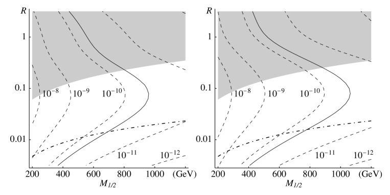
Figure 2: The branching ratio for $\mu\to e\gamma$ in the Type A model with $\tan\beta=2$. The left figure is for $\mu>0$ and the right for $\mu<0$. The solid lines indicate the current experimental bound ($4.9\times 10^{-11}$). The left sides of the solid lines are excluded. The shaded regions are excluded by the real part of the $K^{0}\bar{K}^{0}$ mixing. If the imaginary part of the contribution to the $K^{0}\bar{K}^{0}$ mixing is not suppressed, the excluded regions are extended to the regions above the dot-dashed lines.

Figure 2 displays the branching ratio of $\mu\to e\gamma$ in the case that we use the charge assignment of Type A in Table 1 and only the loop corrections from the gauginos. Why is there a peak around $R\sim 0.1$? The reason is as follows. Remember that the branching ratio is proportional to $\delta m^{2}_{\tilde{e}}/m^{4}_{\tilde{e}}\propto R/(\xi_{\tilde{e}}+e_{R}R)^{2}$. If the slepton mass squared from the gaugino mass, $\xi_{\tilde{e}}M^{2}_{1/2}$, dominates that from the $D$-term, $e_{R}RM^{2}_{1/2}$, we get a smaller branching ratio for a smaller $R$. On the other hand, if the slepton mass from the $D$-term dominates that from the gaugino mass, we get a smaller branching ratio for a larger $R$. The border between two cases must be the around $R\sim\xi_{\tilde{e}}/e_{R}\sim 0.08$. Here we use an anomalous $U(1)$ charge for right-handed scalar muon $e_{2}=2$. This is because the right-handed slepton gives the largest contribution to the branching ratio. This is the reason for the fact that the branching ratio takes its largest value around $R\sim 0.1$.

Figure 3: The branching ratio for $\mu\to e\gamma$ in the Type B model. The meanings of the lines are the same as in Fig. 2.

Figure 3 shows the branching ratio in the case that we take the charge assignment of Type B. Since the main contribution to the $K^{0}\bar{K}^{0}$ mixing is proportional to $\sqrt{\delta_{\tilde{q}}\delta_{\tilde{d}}}$, the constraint on the gaugino mass from the $K^{0}\bar{K}^{0}$ mixing decreases by one order in the case that $\delta_{\tilde{d}}=0$. It can be seen that even the CP violation in $K$ meson does not give a severe constraint. The figure for $\mu>0$ shows that there seems to be a cancellation around $R\sim 1$. Since this charge assignment makes the contribution from the left-handed sleptons vanish, the cancellation between the Feynman diagrams of the right-handed scalar lepton, pointed out in Ref. [31], is realized. For $\mu<0$, the cancellation occurs around $R\sim 3$, though it is not shown in the figure. Even for this weakest constraint, near future experiments can prove the validity of this scenario.

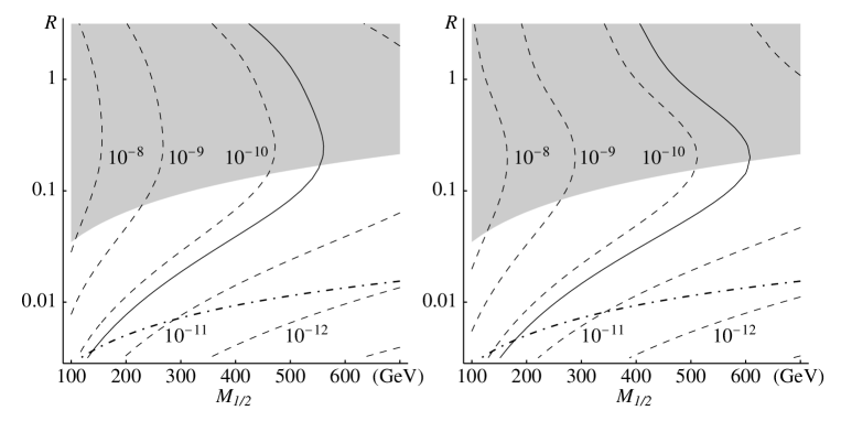
Figure 4: The branching ratio for $\mu\to e\gamma$ with the contribution from the renormalization group from the Planck scale to the GUT scale. Here we adopt the parameters of the minimal $SU(5)$ GUT. The anomalous $U(1)$ charges and the meanings of the lines are the same as in Fig. 2.

As discussed at the end of the previous section, if GUT exists, the renormalization group from the Planck scale, $M_{P}$, to the GUT scale, $M_{G}$, contributes to the sfermion masses. In the case of $SU(5)$ GUT, the contribution is

$$m_{\tilde{f}}^{2}(M_{G}) = m_{\tilde{f}}^{2}(M_{P})+\frac{C^{f}_{5}}{2b_{5}}M_{1/2}^{2}(M_{G})\left[\left(\frac{\alpha_{5}(M_{P})}{\alpha_{5}(M_{G})}\right)^{2}-1\right],$$ (5.5)

$$\sim m_{\tilde{f}}^{2}(M_{P})+\frac{\alpha_{5}(M_{G})}{2\pi}C^{f}_{5}M_{1/2}^{2}(M_{G})\ln\frac{M_{P}}{M_{G}},$$ (5.6)

$$\sim m_{\tilde{f}}^{2}(M_{P})+0.03\times C^{f}_{5}M_{1/2}^{2}(M_{G}),$$ (5.7)

where $C^{f}_{5}$ is the coefficient of the quadratic Casimir ($C^{f}_{5}=72/5$ for the representation ${\bf 10}$ and $C^{f}_{5}=48/5$ for ${\bf 5^{*}}$), and $b_{5}$ is the coefficient of the beta function ($b_{5}=3C(G)+T(R)$). Figure 4 displays the branching ratio in the minimal $SU(5)$ GUT case ($b_{5}=-3$). We can see that a smaller gaugino mass, for example, $M_{1/2}=500$GeV, is allowed. Note that though the amount of the contribution seems to depend on the coefficient of the beta function in Eq. (5.5), there is no difference between the minimal case and the non-minimal case ($b_{5}>-3$) in the approximation to first order in $\displaystyle\frac{\alpha_{5}}{2\pi}\ln(M_{P}/M_{G})$, as in Eq. (5.6). Calculating $m_{\tilde{f}}^{2}(M_{G})$ with no approximation, it can be shown that $m_{\tilde{f}}^{2}(M_{G})$ in the non-minimal cases is slightly larger than that in the minimal case, therefore the constraints on the gaugino mass in Fig. 4 are weakened in the non-minimal cases.

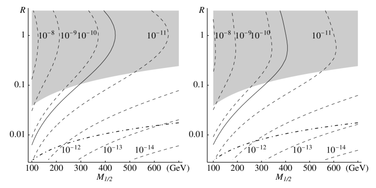
Figure 5: The branching ratio for $\mu\to e\gamma$ with the direct contribution from the $F$-term of the dilaton ($m_{0}^{2}=M^{2}_{1/2}$ at the GUT scale). The anomalous $U(1)$ charges and the meanings of the lines are the same as in Fig. 2.

Figure 5 exhibits the branching ratio in the case that the $F$-term of the dilaton also contributes to the scalar fermion masses directly, as $m_{0}=M_{1/2}$ at the GUT scale. Even if $R=0.1$, the gaugino mass $M_{1/2}>300$GeV is allowed. However, we cannot predict the lowest value of the branching ratio, because the upper limit of the contribution from the dilaton is unknown in this framework.

6 Discussion and Summary

There is a problem in the situation that the gaugino mass dominates sfermion masses ($m_{0}/M_{1/2}\ll 1$) at the GUT scale, as discussed in Ref. [34]. This is that the effective potential is unbounded from below (UFB) and that the standard vacuum in which the electroweak symmetry breaking occurs in a right manner is metastable. In our scenario the ratio of sfermion masses to the gaugino mass $m_{0}/M_{1/2}$ is of the order of $0.3$ for $R\sim 0.1$. According to the analysis in Ref. [34], this ratio means that our scenario is located just around the boundary of the UFB constraint and that the constraint may be satisfied. Even if our scenario does not satisfy it, there is a possibility that the standard vacuum is more stable than the universe. Moreover, if there is another flavor independent contribution to the sfermion masses, such as from GUT interactions or the dilaton, it can be free from this problem since $m_{0}/M_{1/2}\sim 1$.

In this paper, we have studied the case that the dilaton is stabilized by the deformation of the Kähler potential for the dilaton and have pointed out that the order of the ratio of the $F$-term to the $D$-term contributions is generally determined. We estimated FCNC processes from this ratio in this scenario, and we showed that in particular the $\mu\to e\gamma$ process can be around the present experimental upper bound. The analysis in the LANL experiment is expected to make the experimental bound to the branching ratio for $\mu\to e\gamma$ lower to $5\times 10^{-12}$. Moreover, in near future it can be expected that the process is accessible to the branching ratio of the order of $10^{-14}$ [35]. Therefore this process should be observable in the near future if the scenario discussed here is true.

Appendix

In this appendix we briefly give the calculation of the ratio $r$ in Eq. (3.13) for the generalized superpotential (3.11),

$$W = C^{\bar{\imath}_{1},\cdots,\bar{\imath}_{n}}_{i_{1},\cdots,i_{n}}\left(\frac{Q^{i_{1}}\bar{Q}_{\bar{\imath}_{1}}}{M_{P}^{2}}\right)\cdots\left(\frac{Q^{i_{n}}\bar{Q}_{\bar{\imath}_{n}}}{M_{P}^{2}}\right)\left(\frac{\Phi}{M_{P}}\right)^{q_{sum}}M_{P}^{3},$$ (A.1)

where

$$q_{sum}=\sum_{p=1}^{n}(q_{i_{p}}+\bar{q}_{{\bar{\imath}}_{p}}).$$ (A.2)

Below, the dynamical scale $\Lambda$ of the $SU(N_{c})$ gauge theory, the effective superpotential can be written in terms of meson fields $M^{i}_{\bar{\jmath}}\equiv Q^{i}\bar{Q}_{\bar{\jmath}}$ as,

$$W=C^{\bar{\imath}_{1},\cdots,\bar{\imath}_{n}}_{i_{1},\cdots,i_{n}}\left(\frac{M^{i_{1}}_{\bar{\imath}_{1}}}{M_{P}^{2}}\right)\cdots\left(\frac{M^{i_{n}}_{\bar{\imath}_{n}}}{M_{P}^{2}}\right)\left(\frac{\Phi}{M_{P}}\right)^{q_{sum}}M_{P}^{3}+(N_{c}-N_{f})\left(\frac{\Lambda^{3N_{c}-N_{f}}}{\det M}\right)^{\frac{1}{N_{c}-N_{f}}}.$$ (A.3)

On the other hand, since the Kähler potential for the dilaton field $S$ must be a function of $S+S^{\dagger}-\delta_{GS}V^{A}$, because of an anomalous $U(1)$ gauge invariance, the total Kähler potential is

$$K_{tot}=Q^{i}Q^{\dagger}_{i}e^{2q_{i}V^{A}}+\bar{Q}^{\dagger\bar{\imath}}\bar{Q}_{\bar{\imath}}e^{2\bar{q}_{\bar{\imath}}V^{A}}+\Phi^{\dagger}\Phi e^{-2V^{A}}+K(S+S^{\dagger}-\delta_{GS}V^{A}).$$ (A.4)

Along the $SU(N_{c})$ flat direction, the total Kähler potential can be written as

$$K_{tot}=\left(\sqrt{MM^{\dagger}}\right){}^{i}_{i}e^{2q_{i}V^{A}}+\left(\sqrt{M^{\dagger}M}\right){}^{\bar{\imath}}_{\bar{\imath}}e^{2\bar{q}_{\bar{\imath}}V^{A}}+\Phi^{\dagger}\Phi e^{-2V^{A}}+K(S+S^{\dagger}-\delta_{GS}V^{A}).$$ (A.5)

Then

$$\int d^{4}\theta K_{tot} = -D_{A}\left\{q_{i}\left(\sqrt{MM^{\dagger}}\right){}^{i}_{i}+{\bar{q}}_{\bar{\imath}}\left(\sqrt{M^{\dagger}M}\right){}^{\bar{\imath}}_{\bar{\imath}}-|\Phi|^{2}+\xi^{2}\right\}$$ (A.6)

$$+F_{M}{}^{k}_{\bar{k}}F_{M}^{\dagger}{}^{\bar{l}}_{l}(K_{MM^{\dagger}}){}^{\bar{k}}_{k}\;{}^{l}_{\bar{l}}\hskip 5.0pt+\cdots,$$

where

$$(K_{MM^{\dagger}}){}^{\bar{k}}_{k}\;{}^{l}_{\bar{l}}\equiv\frac{\partial^{2}\left\{\mathop{\rm Tr}\nolimits\left(\sqrt{MM^{\dagger}}\right)+\mathop{\rm Tr}\nolimits\left(\sqrt{M^{\dagger}M}\right)\right\}}{\partial M^{k}_{\bar{k}}\partial M^{\dagger}{}^{\bar{l}}_{l}},$$ (A.7)

and $\xi^{2}$ is given by Eq. (2.7). The total scalar potential is

$$V=\frac{1}{K^{\prime\prime}}\left|\frac{\partial W}{\partial S}\right|^{2}+\left|\frac{\partial W}{\partial\Phi}\right|^{2}+\frac{\partial W}{\partial M^{k}_{\bar{k}}}(K^{-1}_{MM^{\dagger}}){}_{\bar{k}}^{k}\;{}_{l}^{\bar{l}}\frac{\partial W^{*}}{\partial M^{\dagger}{}^{k}_{\bar{k}}}+\frac{1}{2g_{A}^{2}}|D_{A}|^{2}.$$ (A.8)

Here we define the parameter $\epsilon\ll 1$ by

$$\epsilon\equiv\left(\frac{\Lambda}{M_{P}}\right)^{\frac{3N_{c}-N_{f}}{nN_{c}-(n-1)N_{f}}},$$ (A.9)

so that we can find a local minimum as an expansion in $\epsilon$:

$$\left\langle\Phi^{2}\right\rangle=\xi^{2}+O(\epsilon).$$ (A.10)

At the minimum, the VEVs of the meson fields are given by the solution of the equations,

$$nC^{\bar{\imath}_{1},\bar{\imath}_{2}\cdots,\bar{\imath}_{n}}_{i_{1},i_{2},\cdots,i_{n}}\left(\frac{M^{i_{2}}_{\bar{\imath}_{2}}}{M_{P}^{2}}\right)\cdots\left(\frac{M^{i_{n}}_{\bar{\imath}_{n}}}{M_{P}^{2}}\right)\left(\frac{\xi}{M_{P}}\right)^{q_{sum}}M_{P}-(M^{-1}){}^{\bar{\imath}_{1}}_{i_{1}}\left(\frac{\Lambda^{3N_{c}-N_{f}}}{\det M}\right)^{\frac{1}{N_{c}-N_{f}}}=0,$$ (A.11)

and the VEVs of the auxiliary fields $D_{A}$ and $F_{S}$ can be written as

$$-\left\langle D_{A}\right\rangle = \epsilon^{2n}\frac{M_{P}^{6}}{\xi^{4}}\left|\frac{1}{\det m}\right|^{\frac{2}{N_{c}-N_{f}}}(2C_{N})^{2}$$ (A.12)

$$\times\left\{\frac{2C_{N}}{N_{c}-N_{f}+\frac{N_{f}}{n}}\left(1-\frac{2K^{\prime}}{\delta_{GS}K^{\prime\prime}}\right)-1\right\},$$

$$\left\langle F_{S}\right\rangle = \epsilon^{n}\frac{M_{P}^{3}}{\xi^{2}}(2C_{N})\frac{K^{\prime}}{K^{\prime\prime}}\left(\frac{1}{\det m^{\dagger}}\right)^{\frac{1}{N_{c}-N_{f}}},$$ (A.13)

where

$$m^{i}_{\bar{\imath}}\equiv\frac{\left\langle M^{i}_{\bar{\imath}}\right\rangle}{\epsilon M_{P}^{2}}.$$ (A.14)

Then the ratio $r\equiv|\left\langle D_{A}\right\rangle|/|\left\langle F_{S}\right\rangle|^{2}$ is

$$r=\frac{1}{N_{c}-N_{f}+\frac{N_{f}}{n}}\frac{4C_{N}}{\delta_{GS}}\left(\frac{K^{\prime\prime}}{-K^{\prime}}\right)+\left\{\frac{2C_{N}}{N_{c}-N_{f}+\frac{N_{f}}{n}}-1\right\}\left(\frac{K^{\prime\prime}}{-K^{\prime}}\right)^{2}.$$ (A.15)

Moreover, we can get the relation among derivatives of the Kähler potential using the minimization condition for the dilaton field $S$:

$$\frac{K^{\prime\prime\prime}}{K^{\prime}}=-\frac{1}{N_{c}-N_{f}+\frac{N_{f}}{n}}\frac{4C_{N}}{\delta_{GS}}\frac{K^{\prime\prime}}{K^{\prime}}\left(1-\frac{\delta_{GS}K^{\prime\prime}}{2K^{\prime}}\right)^{2}+\frac{\delta_{GS}}{2}\left(\frac{K^{\prime\prime}}{K^{\prime}}\right)^{3}.$$ (A.16)

References

- [1] M. Green and J. Schwarz, Phys. Lett. B149 (1984) 117.
- [2] P. Binétruy and E. Dudas, Phys. Lett. B389 (1996) 503.
-
[3]
G. Dvali and A. Pomarol
Phys. Rev. Lett. 77 (1996) 3728;
R.N. Mohapatra and A. Riotto, Phys. Rev. D55 (1997) 1138; Phys. Rev. D55 (1997) 4262. -
[4]
H. Nakano,
hep-th/9404033;
Y. Kawamura and T. Kobayashi, Phys. Lett. B375 (1996) 141; Phys. Rev. D56 (1997) 3844;
E. Dudas, S. Pokorski and C.A. Savoy, Phys. Lett. B369 (1996) 255;
E. Dudas, C. Grojean, S. Pokorski and C.A. Savoy, Nucl. Phys. B481 (1996) 85. - [5] C.D. Froggatt and H.B. Nielsen, Nucl. Phys. B147 (1979) 277.
-
[6]
L. Ibáñez and G.G. Ross,
Phys. Lett. B332 (1994) 100;
P. Binétruy and P. Ramond, Phys. Lett. B350 (1995) 49;
E. Dudas, S. Pokorski and C.A. Savoy, Phys. Lett. B356 (1995) 45;
P. Binétruy, S. Lavignac and P. Ramond, Nucl. Phys. B477 (1996) 353. - [7] A.E. Nelson and D. Wright, Phys. Rev. D56 (1997) 1598.
- [8] Ren-Jie Zhang, Phys. Lett. B402 (1997) 101.
- [9] S. Dimopoulos and G.F. Giudice, Phys. Lett. B357 (1995) 573.
- [10] A.G. Cohen, D.B. Kaplan and A.E. Nelson, Phys. Lett. B388 (1996) 588.
-
[11]
N. Arkani-Hamed and H. Murayama,
Phys. Rev. D56 (1997) 6733;
K. Agashe and M. Graesser, Phys. Rev. D59 (1999) 015007. - [12] N. Arkani-Hamed, M. Dine and S.P. Martin, Phys. Lett. B431 (1998) 329.
- [13] Particle Data Group, Eur. Phys. J. C3 (1998) 1.
-
[14]
E. Witten,
Phys. Lett. B149 (1984) 351;
M. Dine, N. Seiberg and E. Witten, Nucl. Phys. B289 (1987) 589;
J.J. Atick, L.J. Dixon and A. Sen, Nucl. Phys. B292 (1987) 109;
M. Dine, I. Ichinose and N. Seiberg, Nucl. Phys. B293 (1987) 253. - [15] T. Kobayashi and H. Nakano, Nucl. Phys. B496 (1997) 103.
- [16] H. Dreiner, G.K. Leontaris, S. Lola, G.G. Ross and C. Scheich, Nucl. Phys. B436 (1995) 461.
-
[17]
T. Yanagida,
in Proc. of the Workshop on the Unified Theory
and Baryon Number in the Universe, eds.
O. Sawada and A. Sugamoto (KEK report 79-18, 1979);
M. Gell-Mann, P. Ramond and R. Slansky, in Supergravity, eds. P. van Nieuwenhuizen and D.Z. Freedman (North Holland, Amsterdam, 1979). - [18] Z. Maki, M. Nakagawa and S. Sakata, Prog. Theor. Phys. 28 (1962) 870.
- [19] Y. Fukuda et al., Super-Kamiokande Coll., Phys. Rev. Lett. 81 (1998) 1562. For the review, see S.M. Bilenky, C. Giunti and W. Grimus, hep-ph/9812360.
- [20] P. Binétruy, S. Lavignac, S. Petcov and P. Ramond, Nucl. Phys. B496 (1997) 3.
- [21] J. Sato and T. Yanagida, Phys. Lett. B430 (1998) 127; hep-ph/9809307.
- [22] J. Hisano, K. Kurosawa and Y. Nomura, Phys. Lett. B445 (1999) 316.
- [23] T. Barreiro, B. de Carlos, J.A. Casas and J.M. Moreno, Phys. Lett. B445 (1998) 82.
- [24] N. Irges, Phys. Rev. D58 (1998) 115011; hep-ph/9812338.
- [25] I. Affleck, M. Dine and N. Seiberg, Nucl. Phys. B256 (1985) 557.
- [26] A. Kageyama, H. Nakano, T. Ozeki and Y. Watanabe, Prog. Theor. Phys. 101 (1999) 439.
-
[27]
J.S. Hagelin, S. Kelley and T. Tanaka,
Nucl. Phys. B415 (1994) 293;
F. Gabbiani, E. Gabrielli, A. Masiero and L. Silvestrini, Nucl. Phys. B477 (1996) 321. - [28] M.E. Gomez, G.K. Leontaris, S. Lola and J.D. Vergados, Phys. Rev. D59 (1999) 116009.
-
[29]
F. Borzumati and A. Masiero,
Phys. Rev. Lett. 57 (1986) 961;
R. Barbieri and L. Hall, Phys. Lett. B338 (1994) 212;
J. Hisano, T. Moroi, K. Tobe, M. Yamaguchi and T. Yanagida, Phys. Lett. B357 (1995) 579. - [30] J. Hisano, T. Moroi, K. Tobe and M. Yamaguchi, Phys. Rev. D53 (1996) 2442.
- [31] J. Hisano, T. Moroi, K. Tobe and M. Yamaguchi, Phys. Lett. B391 (1997) 341; Erratum-ibid B397 (1997) 357.
- [32] J.A. Bagger, K.T. Matchev and Ren-Jie Zhang, Phys. Lett. B412 (1997) 77.
- [33] M. Ciuchini et al., JHEP 10 (1998) 008.
-
[34]
J.A. Casas, A. Lleyda and C. Muñoz,
Nucl. Phys. B471 (1996) 3;
H. Baer, M. Brihlik and D. Castaño, Phys. Rev. D54 (1996) 6944. -
[35]
Y. Kuno and Y. Okada,
Phys. Rev. Lett. 77 (1996) 434;
Y. Kuno, A. Maki and Y. Okada, Phys. Rev. D55 (1997) 2517.