Finally neutrino has mass

Abstract

The present status of the problem of neutrino mass, mixing and neutrino oscillations is briefly summarized. The evidence for oscillations of atmospheric neutrinos found recently in the Super-Kamiokande experiment is discussed. Indications in favor of neutrino oscillations obtained in solar neutrino experiments and in the accelerator LSND experiment are also considered. Implications of existing neutrino oscillation data for neutrino masses and mixing are discussed.

I Introduction

The Glashow-Weinberg-Salam [1] theory of electroweak interactions, which combined with the Quantum Chromo-Dynamics (QCD) is now called the Standard Model (SM), is one of the greatest achievements of particle physics in the 20^th century. Among others, the Glashow-Weinberg-Salam theory allowed to predict successfully the existence of charmed-particles [2], of the $b$ and $t$ quarks, a new class of weak interactions (neutral currents), the existence of the vector $W^{\pm}$ and $Z^{0}$ bosons and their masses. All the predictions of the SM have been confirmed by numerous experiments; the theory describes beautifully all the existing experimental data in the whole energy range available at present (except for the indications in favor of neutrino oscillations that we will discuss in the following).

However, the prevailing general consensus is that the SM cannot be the final theory of elementary particles. The SM is a theory of weak, electromagnetic and strong interactions with the exception of gravity. In this theory, more than 20 arbitrary fundamental parameters (masses of quarks and leptons, coupling constants, mixing angles, etc.) still remain to be explained. Also, there are several conceptual problems; to name only two, the lack of any explanation of why in nature there exist three generations of quarks and leptons that differ only in masses and the hierarchy problem, connected with the radiative corrections to the mass of the Higgs boson.

Major efforts at the moment are directed towards the search for a theory of elementary particles that could generalize the SM and would solve the problems mentioned above. In the past, many such models have been proposed. They include, among others, Grand Unified models, Supersymmetric models, Superstring models, composite models [3]. In many experiments, possible effects of physics beyond the Standard Model have been and will be searched for. In the frontier of accelerator high energy experiments, one of the major goals is to find, as a signature of new physics, supersymmetric particles or some unexpected behavior of the standard Higgs boson. Among accelerator and non-accelerator physics experiments, one of the most popular searches have been that of neutrino masses via neutrino oscillations, for most theories beyond the SM predict non-zero neutrino masses, and that of proton decay. At present some evidence on new physics beyond the SM has been found only in neutrino oscillation experiments.

If neutrinos are massive and mixed, the states of flavor neutrinos $\nu_{e}$, $\nu_{\mu}$, $\nu_{\tau}$ are mixed coherent superpositions of the states of neutrinos with definite mass. In this case, neutrinos produced via weak interactions experience neutrino oscillations, which are periodical transitions among different flavor neutrinos. Such effects appear to have been observed in several neutrino experiments.

An impressive evidence for the disappearance of atmospheric $\nu_{\mu}$’s has been presented by the Super-Kamiokande collaboration [4, 5, 6, 7, 8]. Similar indications in favor of neutrino oscillations have also been obtained in the Kamiokande [9], IMB [10], Soudan 2 [11] and MACRO [12] atmospheric neutrino experiments. All the existing data of solar neutrino experiments (Homestake [13], Kamiokande [14], GALLEX [15], SAGE [16], Super-Kamiokande [17, 8]) can naturally be explained by neutrino mass and mixing. Finally, some indication in favor of $\bar{\nu}_{\mu}\to\bar{\nu}_{e}$ and $\nu_{\mu}\to\nu_{e}$ oscillations has been found in the accelerator LSND experiment [18, 19].

These data constitute the first observation of processes in which lepton numbers are not conserved. It is a general belief that such phenomena are due to physics beyond the SM [20].

The purpose of this article is to review the theory and phenomenology of neutrino masses, neutrino mixing and the salient features of neutrino oscillations. In Section II, a short discussion of the theory of two-component neutrinos, the Standard Model and the law of conservation of lepton numbers will be given. In Section III, we will consider the problem of neutrino mass and different possibilities of neutrino mixing. Neutrino oscillations will be discussed in Section IV and the experimental data will be briefly presented and discussed in Section V. Conclusions are drawn in Section VI.

II Two-component neutrino, Standard Model and lepton numbers

In 1957, soon after the discovery of parity violation in weak interactions (Wu et al. [21]) Landau [22], Lee and Yang [23] and Salam [24] proposed the theory of two-component massless neutrinos.

Starting with the field $\nu(x)$ of the neutrino with mass $m$, which satisfies the Dirac equation

$$(i\gamma^{\alpha}\partial_{\alpha}-m)\ \nu=0\,,$$ (1)

let us introduce the left-handed $\nu_{L}$ and right-handed $\nu_{R}$ components of the neutrino field, respectively, as

$$\nu_{L,R}=\frac{1\mp\gamma_{5}}{2}\ \nu\,.$$ (2)

From (1), for $\nu_{L,R}$ we have a set of coupled equations,

$$i\gamma^{\alpha}\partial_{\alpha}\nu_{L}-m\nu_{R}=0\,,$$ (3)

$$i\gamma^{\alpha}\partial_{\alpha}\nu_{R}-m\nu_{L}=0\,.$$ (4)

If the neutrino mass is zero, the equations for $\nu_{L}$ and $\nu_{R}$ are decoupled,

$$i\gamma^{\alpha}\partial_{\alpha}\nu_{L}=0\,,\qquad i\gamma^{\alpha}\partial_{\alpha}\nu_{R}=0\,,$$ (5)

and the left-handed component $\nu_{L}$ (or right-handed component $\nu_{R}$) can be chosen as the neutrino field. This was the choice of the authors of the two-component neutrino theory.

If the neutrino field is $\nu_{L}$, a neutrino with definite momentum has negative helicity (projection of spin on the direction of the momentum) and an antineutrino has positive helicity (see Fig. 1). If the neutrino field is $\nu_{R}$, a neutrino has positive helicity and an antineutrino has negative helicity.

FIG. 1.: Helicities of two component neutrino and antineutrinos described by the field $\nu_{L}$. The direction of momentum (thin arrows) and spin (thick arrows) are shown.

The two-component neutrino theory was confirmed in the famous Goldhaber et al. experiment [25] (1958), in which the helicity of neutrino was determined from the measurement of circular polarization of the photon in the process

$$e^{-}+\mathrm{Eu}\to\nu_{e}+\hbox{} \mathrm{Sm}^{*}$$ (6)

$$\downarrow$$ (7)

$$\mathrm{Sm} \hbox{}+\gamma\,.$$ (8)

The measured circular polarization was consistent with a neutrino with negative helicity.

The phenomenological $V-A$ theory of weak interactions by Feynman and Gell-Mann [26] and Sudarshan and Marshak [27] was based on the assumption that only the left-handed components of all fields are involved in the Hamiltonian of weak interactions. Assuming also the universality of the weak interactions, Feynman and Gell-Mann in 1958 proposed a Hamiltonian that is a product of two currents

$$\mathcal{H}_{I}^{\mathrm{CC}}=\frac{G_{\mathrm{F}}}{\sqrt{2}}\ j^{\mathrm{CC}\alpha}\ {j^{\mathrm{CC}}_{\alpha}}^{\dagger}\,,$$ (9)

which was successful in describing all the existing weak interaction data. In Eq.(9), $j_{\alpha}^{\mathrm{CC}}$ is the charged weak current (see later) and $G_{\mathrm{F}}$ is the Fermi constant.

The SM is based on a spontaneously broken $SU(2)\times U(1)$ local gauge group with the left-handed doublets

$$\left(\begin{array}[]{c}\nu_{e}\\ e\end{array}\right)_{L}\,,\qquad\left(\begin{array}[]{c}\nu_{\mu}\\ \mu\end{array}\right)_{L}\,,\qquad\left(\begin{array}[]{c}\nu_{\tau}\\ \tau\end{array}\right)_{L}\,,$$ (10)

and the right-handed singlets $e_{R}$, $\mu_{R}$ and $\tau_{R}$ (we are interested here only in the lepton part of the SM).

The interactions of leptons and vector bosons in the SM has three parts:

1. The Hamiltonian of electromagnetic interaction

   $$\mathcal{H}_{I}^{\mathrm{em}}=e\ j^{\mathrm{em}}_{\alpha}\ A^{\alpha}\,,$$ (11)

   where $A_{\alpha}$ is the electromagnetic field, $e$ is the electric charge and

   $$j^{\mathrm{em}}_{\alpha}=\bar{e}\gamma_{\alpha}e+\bar{\mu}\gamma_{\alpha}\mu+\bar{\tau}\gamma_{\alpha}\tau$$ (12)

   is the electromagnetic current;

2. The Hamiltonian of charged current (CC) weak interactions

   $$\mathcal{H}_{I}^{\mathrm{CC}}=\frac{g}{2\sqrt{2}}\ j^{\mathrm{CC}}_{\alpha}\ W^{\alpha}+\mathrm{h.c.}\,,$$ (13)

   where $g$ is an interaction constant, $W^{\alpha}$ is the field of charged vector bosons, and

   $$j^{\mathrm{CC}}_{\alpha}=2\left(\bar{e}_{L}\gamma_{\alpha}\nu_{eL}+\bar{\mu}_{L}\gamma_{\alpha}\nu_{\mu L}+\bar{\tau}_{L}\gamma_{\alpha}\nu_{\tau L}\right)$$ (14)

   is the charged current;

3. The Hamiltonian of neutral current (NC) weak interactions

   $$\mathcal{H}_{I}^{\mathrm{NC}}=\frac{g}{2\cos{\vartheta_{\mathrm{W}}}}\ j^{\mathrm{NC}}_{\alpha}\ Z^{\alpha}\,,$$ (15)

   where $\vartheta_{\mathrm{W}}$ is the weak (Weinberg) angle, $Z^{\alpha}$ is the field of the neutral vector boson, and

   $$j^{\mathrm{NC}}_{\alpha}=\bar{\nu}_{eL}\gamma_{\alpha}\nu_{eL}+\bar{\nu}_{\mu L}\gamma_{\alpha}\nu_{\mu L}+\bar{\nu}_{\tau L}\gamma_{\alpha}\nu_{\tau L}+\ldots$$ (16)

   is the neutral current.

The three fields of $\nu_{e}$, $\nu_{\mu}$ and $\nu_{\tau}$ enter in the standard charged and neutral currents (14) and (16). There exist no light flavor neutrinos other than these. This was impressively proved by the measurement of the width of the decay $Z\to\nu+\bar{\nu}$ in the SLC and LEP experiments [28]. In the framework of the SM, the width is determined only by the number $N_{\nu}$ of light flavor neutrinos. In the recent LEP experiments, this number was found to be

$$N_{\nu}=2.994\pm 0.011\,.$$ (17)

	$(\nu_{e},~{}e^{-})$	$(\nu_{\mu},~{}\mu^{-})$	$(\nu_{\tau},~{}\tau^{-})$
$L_{e}$	1	0	0
$L_{\mu}$	0	1	0
$L_{\tau}$	0	0	1

TABLE I.: Lepton numbers of neutrinos and charged leptons

The three different types of neutrinos are distinguished by the values of three different conserved lepton numbers: electron $L_{e}$, muon $L_{\mu}$ and tau $L_{\tau}$ (see Table I). Zero lepton numbers are assigned to quarks, $\gamma$, $W$, $Z$, etc.. The SM interactions (11), (13), (15) conserve separately the total electron, muon and tau lepton numbers:

$$\sum L_{e}=\mathrm{const}\,,\qquad\sum L_{\mu}=\mathrm{const}\,,\qquad\sum L_{\tau}=\mathrm{const}\,.$$ (18)

Up to now, there is no indication of a violation of this conservation law in weak interaction processes as weak decays, neutrino interactions, etc.. From the existing data, rather strong limits on the probabilities of the processes that are forbidden by (18) have been obtained:

$$\Gamma(\mu\to e\,\gamma)/\Gamma(\mu\to\mathrm{all})<4.9\times 10^{-11}\,,$$ (19)

$$\Gamma(\mu\to 3\,e)/\Gamma(\mu\to\mathrm{all})<1.0\times 10^{-12}\,,$$ (20)

$$\sigma(\mu^{-}\,\mathrm{Ti}\to e^{-}\,\mathrm{Ti})/\sigma(\mu^{-}\,\mathrm{Ti}\to\mathrm{capture})<4.3\times 10^{-12}\,,$$ (21)

$$\Gamma(K_{L}\to e\,\mu)/\Gamma(K_{L}\to\mathrm{all})<3.3\times 10^{-11}\,,$$ (22)

$$\Gamma(K^{+}\to\pi^{+}\,e^{-}\,\mu^{+})/\Gamma(K^{+}\to\mathrm{all})<2.1\times 10^{-10}\,,$$ (23)

at 90% CL [28].

In spite of the above impressive data, modern gauge theories suggest that the lepton number conservation law is only approximate. It is violated if neutrinos are massive and mixed. In the next Section we will discuss neutrino masses and neutrino mixings with emphasis on how, as a consequence, the law of lepton number conservation is violated.

III Neutrino mass and mixings

The fields of $d$, $s$, $b$ quarks with charge $-1/3$ (“down quarks”) enter in the charged current of the SM in a mixed form. The quark charged current is

$$j^{\mathrm{CC}}_{\alpha}=2\left(\bar{u}_{L}\gamma_{\alpha}d^{\prime}_{L}+\bar{c}_{L}\gamma_{\alpha}s^{\prime}_{L}+\bar{t}_{L}\gamma_{\alpha}b^{\prime}_{L}\right)\,,$$ (24)

where

$$d^{\prime}_{L}=\sum_{q=d,s,b}V_{uq}\ q_{L}\,,\qquad s^{\prime}_{L}=\sum_{q=d,s,b}V_{cq}\ q_{L}\,,\qquad b^{\prime}_{L}=\sum_{q=d,s,b}V_{tq}\ q_{L}\,.$$ (25)

Here $u$, $c$, $t$ are the fields of the quarks with charge $2/3$ (“up quarks”) and $V$ is the unitary Cabibbo-Kobayashi-Maskawa (CKM) mixing matrix [29].

Quark mixing is a well-established phenomenon. The values of the elements of the CKM matrix have been determined from the results of many experiments and are known with a high accuracy [28]. Quark mixing is a possible source of the CP-violation observed in the decays of neutral K-mesons [30] through the phase which enters in the CKM mixing matrix.

What about neutrinos? Are neutrinos massive and, if so, do the fields of massive neutrinos, like the fields of quarks, enter into the lepton charged current in a mixed form? The answer to these questions is of fundamental importance for particle physics.

The following upper bounds have been obtained in the experiments on the direct measurement of the masses of neutrinos:

$$m_{\nu_{e}}\lesssim 3\,\mathrm{eV} \mathrm{(90\%\,CL)}\,,$$ (26)

$$m_{\nu_{\mu}}<170\,\mathrm{keV} \mathrm{(90\%\,CL)}\,,$$ (27)

$$m_{\nu_{\tau}}<18.2\,\mathrm{MeV} \mathrm{(95\%\,CL)}\,.$$ (28)

The upper bound for the $\nu_{e}$ mass was obtained from the experiments on the measurement of high energy part of the $\beta$-spectrum of ³H-decay [31]. The upper bound for the $\nu_{\mu}$ mass comes from the experiments on the measurement of muon momentum in the decay $\pi^{+}\to\mu^{+}\nu_{\mu}$ [32] and the upper bound for the $\nu_{\tau}$ mass from experiments on the measurement of the distribution of effective mass of five pions in the decay $\tau\to\nu_{\tau}+5\pi$ [33].

Although these data do not exclude massless neutrinos, there are no convincing reasons for massless neutrinos. Moreover, in theories such as Grand Unified gauge theories, for example, it is very natural for neutrinos to be massive particles: the non-conservation of lepton numbers and the appearance of right-handed neutrino fields in the Lagrangian are generic features of these theories.

From all the existing neutrino data and from the astrophysical constraints [28] we can expect, however, that neutrino masses are small. To probe hard-to-find effects of small neutrino masses, it requires some very sensitive special experiments. Such experiments have turned out to be neutrino oscillation experiments. Before we discuss neutrino oscillations in detail in the following Sections, we will first discuss different possibilities of mixing of massive neutrinos.

As mentioned already, the minimal Standard Model is based on the assumption that neutrino fields are left-handed two-component fields and there are no right-handed fields in the Lagrangian. In such a model, neutrinos are two-component massless particles (as in Fig. 1).

Neutrino masses can be generated, however, by the same standard Higgs mechanism which generates the masses of quarks and charged leptons, due to Yukawa interactions of neutrinos with the Higgs boson. This interaction requires not only the left-handed doublets (10), but also right-handed singlets $\nu_{\ell R}$. In this case, the neutrino mass term is given by

$$\mathcal{L}=-\sum_{\ell^{\prime},\ell}\bar{\nu}_{\ell^{\prime}R}\ M_{\ell^{\prime}\ell}\ \nu_{\ell L}+\mathrm{h.c.}\,,$$ (29)

where $M$ is a complex matrix. If $M$ is non-diagonal, this Lagrangian does not conserve the lepton numbers and the flavor neutrino fields $\nu_{eL}$, $\nu_{\mu L}$, $\nu_{\tau L}$ are given by

$$\nu_{\ell L}=\sum_{i=1}^{3}U_{\ell i}\ \nu_{iL}\qquad(\ell=e,\mu,\tau)\,.$$ (30)

Here $\nu_{i}$ is the field of the neutrino with mass $m_{i}$ and $U$ is the unitary mixing matrix.

The mass term (29) does not conserve the lepton numbers $L_{e}$, $L_{\mu}$ and $L_{\tau}$ separately, but it conserves the total lepton number

$$L=L_{e}+L_{\mu}+L_{\tau}$$ (31)

and the neutrinos $\nu_{i}$ with definite mass are four component Dirac particles (neutrinos and antineutrinos have, correspondingly, $L=1$ and $L=-1$).

If Dirac neutrino masses are generated by the same mechanism as quark and charged lepton masses, the neutrino masses are only additional parameters of the SM and there is no rationale for the smallness of neutrino masses compared with the masses of the corresponding charged leptons.

A mechanism that explains the smallness of neutrino masses exists if the neutrinos $\nu_{i}$ with definite masses are two-component Majorana particles. It is the famous see-saw mechanism of neutrino mass generation [34]. The see-saw mechanism is based on the assumption that all lepton numbers are violated at a scale $M$ that is much larger than the electroweak scale (usually $M\sim 10^{16}\,\mathrm{GeV}$). For the neutrino mixing, we have the same expression as (30), but in this case the field of neutrino with mass $m_{i}$ satisfies the Majorana condition

$$\nu_{i}^{c}=\nu_{i}$$ (32)

($\nu_{i}^{c}$ is the charge-conjugated field) and the value of the neutrino mass $m_{i}$ is given by the see-saw relation

$$m_{i}\simeq\frac{(m_{f}^{i})^{2}}{M}\,.$$ (33)

Here $m_{f}^{i}$ is the mass of up-quark or lepton in the $i^{\mathrm{th}}$-generation.

Massive Majorana neutrinos are truly neutral particles that have no lepton charge (neutrinos are identical to antineutrinos). Majorana neutrino masses can be generated only in the framework of models beyond the SM in which the conservation of the total lepton number is violated.

If massive neutrinos are Majorana particles, the number of massive light neutrinos can be larger than three (the number of flavor neutrinos). In this case, we have

$$\nu_{\ell L}=\sum_{i=1}^{n}U_{\ell i}\ \nu_{iL}\,,\qquad\nu_{sL}=\sum_{i=1}^{n}U_{si}\ \nu_{iL}\,,$$ (34)

where $\nu_{s}$ is the charge conjugated right-handed field ($\nu_{sL}={\nu_{sR}}^{c}$) and $n=3+n_{s}$, where $n_{s}$ is the number of sterile neutrinos.

Right-handed neutrino fields do not enter into the charged and neutral currents of the SM (see Eqs.(13) and (15)). This means that the quanta of the neutrino fields $\nu_{s}$ do not interact with matter (via the standard weak interaction). Such neutrinos are called sterile neutrinos. Because of neutrino mixing, the flavor neutrinos $\nu_{e}$, $\nu_{\mu}$ and $\nu_{\tau}$ can transform into sterile states. Such a possibility is widely discussed now in the literature in order to accommodate all the existing neutrino oscillation data.

Some important questions that are currently under active investigation are:

1. What are the values of neutrino masses?

2. What are the values of the elements of the unitary neutrino mixing matrix $U$ ?

3. What is the nature of massive neutrinos? Are they Dirac particles with total lepton number equal to $1$ ($-1$) or truly neutral Majorana particles with zero lepton number?

4. Are there transitions of active neutrinos into sterile states?

5. Is CP violated in the lepton sector?

Many experiments designed to observe neutrino oscillations, to investigate neutrinoless double $\beta$-decay

$$(A,Z)\to(A,Z+2)+e^{-}+e^{-}\,,$$ (35)

and to perform a precise measurement of the high-energy part of the $\beta$-spectrum of ³H-decay are all aimed to answer these fundamental questions. As we will see in the next Section, neutrino oscillations provide a unique opportunity to reveal the effects of extremely small neutrino masses and small mixing.

IV Neutrino oscillations

If neutrinos have small mass and are mixed particles, neutrino oscillations take place [35, 36]. Neutrino oscillations were considered as early as in 1957 by B. Pontecorvo [37] and flavor neutrino mixings has been discussed in 1962 by Maki, Nakagawa and Sakata [38].

In this Section, we will discuss neutrino oscillations in some detail. From the quantum mechanical point of view, neutrino oscillations are similar to the very well-known oscillations of neutral kaons $K^{0}\rightleftarrows\bar{K}^{0}$. Let us consider a beam of neutrinos with momentum $p$. In the case of neutrino mixing ((30) or (34)), the state of a neutrino $|\nu_{\ell}\rangle$ ($\ell=e,\mu,\tau$) produced in a weak process (for example, $\pi\to\mu\nu_{\mu}$, $n\to pe^{-}{\bar{\nu}}_{e}$, etc.) is a coherent superposition of the states of neutrinos with definite mass,

$$|\nu_{\ell}\rangle=\sum_{i}U^{*}_{\ell i}\ |\nu_{i}\rangle\,,$$ (36)

where $|\nu_{i}\rangle$ is the state of a neutrino with momentum $p$ and energy

$$E_{i}=\sqrt{p^{2}+m^{2}_{i}}\simeq{p+\frac{m_{i}^{2}}{2p}}\,.$$ (37)

At the time $t$ after production, the neutrino is no longer described by a pure flavor state, but by the state

$$|\nu_{\ell}\rangle_{t}=\sum_{i}U^{*}_{\ell i}\ e^{-iE_{i}t}\ |\nu_{i}\rangle\,.$$ (38)

Neutrinos can only be detected via weak interaction processes. Decomposing the state $|\nu_{\ell}\rangle_{t}$ in terms of weak eigenstates $|\nu_{\ell^{\prime}}\rangle$, we have

$$|\nu_{\ell}\rangle_{t}=\sum_{\ell^{\prime}}|\nu_{\ell^{\prime}}\rangle\ \mathcal{A}_{\nu_{\ell^{\prime}};\nu_{\ell}}(t)\,,$$ (39)

where

$$\mathcal{A}_{\nu_{\ell^{\prime}};\nu_{\ell}}(t)=\sum_{i}U_{\ell^{\prime}i}\ e^{-iE_{i}t}\ U_{\ell i}^{*}\,.$$ (40)

Thus, if neutrino mixing takes place, the state of a neutrino produced at $t=0$ as a state with definite flavor becomes at the time $t>0$ a superposition of all possible states of flavor neutrinos. The quantity $\mathcal{A}_{\nu_{\ell^{\prime}};\nu_{\ell}}(t)$ is the amplitude of the transition $\nu_{\ell}\to\nu_{\ell^{\prime}}$ during the time $t$. It is clear from Eq.(40) that the transitions among different neutrino flavors are effects of the phase differences of the different mass components of the flavor state. For the transition probability we have

$$P_{\nu_{\alpha}\to\nu_{\alpha^{\prime}}}=\left|\sum_{i}U_{\alpha^{\prime}i}^{*}\ U_{\alpha i}\left[\exp\left(-i\ \frac{\Delta{m}^{2}_{i1}L}{2p}\right)-1\right]+\delta_{\alpha^{\prime}\alpha}\right|^{2}\,,$$ (41)

where $\Delta{m}^{2}_{ij}\equiv m_{i}^{2}-m_{j}^{2}$ and $L\simeq t$ is the distance between the neutrino production and detection points.

The expression (41) is valid not only for the transitions among flavor neutrinos $\nu_{e}$, $\nu_{\mu}$, $\nu_{\tau}$ but also for the transitions of flavor neutrinos into sterile states $\nu_{s}$. In this case the index $i$ runs over $n>3$ values ($n$ is the number of massive neutrinos) and the indexes $\alpha^{\prime}$, $\alpha$ run over $e$, $\mu$, $\tau$, $s_{1}$, $\ldots$.

As one can see from Eq.(41), the transition probabilities depend on the parameter $L/p$, on $n-1$ neutrino mass squared differences and on the elements of the neutrino mixing matrix, that can be parameterized in terms of $n(n-1)/2$ mixing angles and $(n-1)(n-2)/2$ phases. If all $\Delta{m}^{2}_{i1}$ are so small that the inequalities

$$\frac{\Delta{m}^{2}_{i1}L}{2p}\ll 1$$ (42)

are satisfied, we simply have $P_{\nu_{\alpha}\to\nu_{\alpha^{\prime}}}=\delta_{\alpha\alpha^{\prime}}$ and neutrino oscillations do not take place.

Let us consider the simplest case of mixing of two types of neutrinos. In this case we have

$$\nu_{\alpha L}=\cos{\vartheta}\ \nu_{1L}+\sin{\vartheta}\ \nu_{2L}$$ (43)

$$\nu_{\alpha^{\prime}L}=-\sin{\vartheta}\ \nu_{1L}+\cos{\vartheta}\ \nu_{2L}\,,$$ (44)

where $\vartheta$ is the mixing angle and $\alpha$, $\alpha^{\prime}$ take the values $\mu,e$, or $\mu,\tau$, or $e,\tau$, or $\mu,s$, etc.. From Eq.(41), the transition probabilities are given by

$$P_{\nu_{\alpha}\to\nu_{\alpha^{\prime}}}=\frac{1}{2}\ \sin^{2}{2\vartheta}\left(1-\cos\frac{\Delta{m}^{2}L}{2p}\right)\qquad\qquad(\alpha^{\prime}\neq\alpha)$$ (45)

$$P_{\nu_{\alpha}\to\nu_{\alpha}}=1-P_{\nu_{\alpha}\to\nu_{\alpha^{\prime}}}=1-\frac{1}{2}\ \sin^{2}{2\vartheta}\left(1-\cos\frac{\Delta{m}^{2}L}{2p}\right)\,,$$ (46)

where $\Delta{m}^{2}\equiv m^{2}_{2}-m^{2}_{1}$. The probability $P_{\nu_{\alpha}\to\nu_{\alpha^{\prime}}}$ can also be written in the form

$$P_{\nu_{\alpha}\to\nu_{\alpha^{\prime}}}=\frac{1}{2}\ \sin^{2}{2\vartheta}\left[1-\cos\left(2.48\ \frac{\Delta{m}^{2}L}{E}\right)\right]\,,$$ (47)

where $\Delta{m}^{2}$ is the neutrino mass squared difference in units of eV², $L$ is the distance in m (km) and $E$ is neutrino energy in MeV (GeV). The mixing parameter $\sin^{2}{2\vartheta}$ is the oscillation amplitude. Thus, for a fixed energy, the transition probability is a periodical function of the distance. The oscillation length $L_{\mathrm{osc}}$ that characterizes this periodicity is given by

$$L_{\mathrm{osc}}=4\pi\ \frac{E}{\Delta{m}^{2}}=2.54\ \frac{E\ (\mathrm{MeV})}{\Delta{m}^{2}\ (\mathrm{eV}^{2})}\ \mathrm{m}\,.$$ (48)

The transition probabilities among different neutrino flavors depend on the parameter $L/E$. This oscillatory behavior is shown in Fig. 2 for $\sin^{2}2\vartheta=1$ and $\Delta{m}^{2}=10^{-3}\,\mathrm{eV}^{2}$ (grey line).

In practice, neutrino beams are not monoenergetic and neutrino sources and detectors have always a finite size. The black curve in Fig. 2 shows the effects of averaging of the transition probability over a Gaussian neutrino spectrum with a mean energy value $\overline{E}=E$ and a standard deviation $\sigma=E/10$.

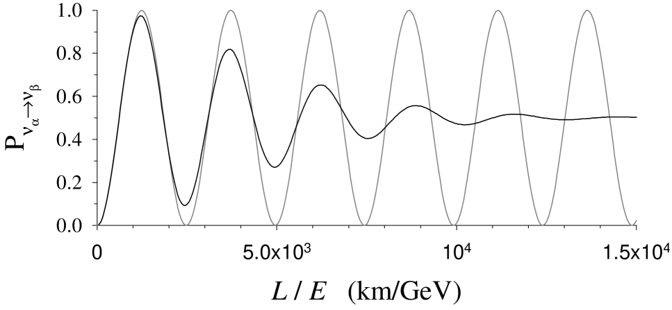
FIG. 2.: Transition probability for $\sin^{2}2\vartheta=1$ and $\Delta{m}^{2}=10^{-3}\,\mathrm{eV}^{2}$ as a function of $L/E$ in km/GeV (or m/MeV). The grey line represents the transition probability (47) and the black line represents the same transition probability averaged over a Gaussian energy spectrum with a mean energy value $\overline{E}=E$ and standard deviation $\sigma=E/10$.

In order to observe neutrino oscillations it is necessary that the neutrino mass squared difference $\Delta{m}^{2}$ satisfies the condition

$$\Delta{m}^{2}\gtrsim\frac{E}{L}\,.$$ (49)

This condition provides a guideline for finding the sensitivity of neutrino oscillation experiments to the neutrino mass squared difference (for large values of $\sin^{2}{2\vartheta}$). For example, for reactor ($L\sim 100\,\mathrm{m}$, $E\sim 1\,\mathrm{MeV}$), accelerator ($L\sim 1\,\mathrm{km}$, $E\sim 1\,\mathrm{GeV}$) and solar ($L\sim 10^{11}\,\mathrm{m}$, $E\sim 1\,\mathrm{MeV}$) neutrino oscillation experiments, the minimal values of $\Delta{m}^{2}$ are $\sim 10^{-2}\,\mathrm{eV}^{2}$, $\sim 1\,\mathrm{eV}^{2}$, $\sim 10^{-11}\,\mathrm{eV}^{2}$, respectively. However, in order to calculate precisely the sensitivity of neutrino oscillation experiments, it is necessary to take into account also all the conditions of an experiment.

A typical exclusion plot in the $\sin^{2}2\vartheta$–$\Delta{m}^{2}$ plane, obtained from the data of experiments in which neutrino oscillations were not found, is presented in Fig. 3 [39]. This plot shows the exclusion curves in the $\nu_{\mu}\to\nu_{\tau}$ channel obtained in the CDHS [40], FNAL E531 [41], CHARM II [42], CCFR [43], CHORUS [44] and NOMAD [45, 39] accelerator experiments. The excluded region lies on the right of the curves.

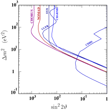
FIG. 3.: Exclusion curves (90% CL) in the $\nu_{\mu}\to\nu_{\tau}$ channel obtained in the CDHS [40], FNAL E531 [41], CHARM II [42], CCFR [43], CHORUS [44] and NOMAD [45, 39] experiments.

The expressions (45) and (46) that describe neutrino oscillations between two types of neutrinos are usually employed in the analysis of experimental data. The general expressions for the transition probabilities among three types of neutrinos are rather complicated, but the probabilities become simple if there is a hierarchy of neutrino masses,

$$m_{1}\ll m_{2}\ll m_{3}\,.$$ (50)

Such a hierarchy is realized, for example, if neutrino masses are generated by the see-saw mechanism.

In the case of a mass hierarchy the $\nu_{\alpha}\to\nu_{\alpha}^{\prime}$ transition probability and the $\nu_{\alpha}\to\nu_{\alpha}$ survival probability in neutrino oscillation experiments for which only the largest mass-squared $\Delta{m}^{2}_{31}$ is relevant are given by [46]

$$P_{\nu_{\alpha}\to\nu_{\alpha^{\prime}}}=\frac{1}{2}\ A_{\alpha;\alpha^{\prime}}\left(1-\cos\frac{\Delta{m}^{2}_{31}L}{2p}\right)\qquad\qquad(\alpha^{\prime}\neq\alpha)\,,$$ (51)

$$P_{\nu_{\alpha}\to\nu_{\alpha}}=1-\frac{1}{2}\ B_{\alpha;\alpha}\left(1-\cos\frac{\Delta{m}^{2}_{31}L}{2p}\right)\,,$$ (52)

with the oscillation amplitudes

$$A_{\alpha;\alpha^{\prime}}=4\ |U_{\alpha 3}|^{2}\ |U_{\alpha^{\prime}3}|^{2}\,,\qquad B_{\alpha;\alpha}=4\ |U_{\alpha 3}|^{2}\ (1-|U_{\alpha 3}|^{2})\,.$$ (53)

The expressions (51) and (52) have the same form as the two-neutrino expressions (45) and (46), respectively. They describe, however, all possible transitions among three types of neutrinos: $\nu_{\mu}\leftrightarrows\nu_{e}$, $\nu_{\mu}\leftrightarrows\nu_{\tau}$ and $\nu_{e}\leftrightarrows\nu_{\tau}$.

The transition probabilities (51) and (52) are characterized by the two mixing parameters $|U_{e3}|^{2}$ and $|U_{\mu 3}|^{2}$ (from the unitarity of the mixing matrix it follows that $|U_{\tau 3}|^{2}=1-|U_{e3}|^{2}-|U_{\mu 3}|^{2}$) and by one neutrino mass-squared difference $\Delta{m}^{2}_{31}\equiv m_{3}^{2}-m_{1}^{2}$. The expressions (51) and (52) are currently often used in the analysis of data of reactor, accelerator and atmospheric neutrino oscillation experiments [47].

There are two types of oscillation experiments:

1. Appearance experiments;

2. Disappearance experiments.

In the experiments of the first type, neutrinos of a certain flavor (for example, $\nu_{\mu}$) are produced and then the appearance of neutrinos of a different flavor (for example, $\nu_{\tau}$) are searched for at some distance. In the experiments of the second type, neutrinos of a certain flavor (say, $\nu_{\mu}$) are produced and, at some distance, neutrinos of the same flavor ($\nu_{\mu}$) are detected. In the latter case, if the number of detected neutrino events is less than the expected number (with the assumption that there are no oscillations), one has a signal that some neutrinos are transformed into neutrinos of other flavors. Reactor neutrino experiments in which $\bar{\nu}_{e}\to\bar{\nu}_{e}$ transitions are searched for are typical disappearance experiments. Accelerator neutrino oscillation experiments can be both of appearance and of disappearance type.

In the next Section we will discuss some results of neutrino oscillation experiments.

V Status of neutrino oscillations

The first experimental information on neutrino oscillations have been obtained about twenty years ago as a by-product of an experiment designed for other measurements. At present, the majority of neutrino experiments are dedicated to the detection of neutrino oscillations.

An impressive evidence in favor of oscillations of atmospheric neutrinos has been obtained recently in the Super-Kamiokande experiment [4, 5, 6, 7, 8]. The results of this experiment reported at the Neutrino ’98 conference [48] attracted enormous attention to the problem of neutrino mass from the general public as well as from many physicists.

Indications in favor of neutrino oscillations have been obtained also in the Kamiokande [9], IMB [10], Soudan 2 [11] and MACRO [12] atmospheric neutrino experiments. In all the solar neutrino experiments (Homestake [13], Kamiokande [14], GALLEX [15], SAGE [16], Super-Kamiokande [17, 8]) the observed event rates are significantly smaller than the expected ones. This solar neutrino problem can naturally be explained if neutrinos are massive and mixed. Indications in favor of neutrino oscillations were also found in the accelerator LSND neutrino experiment [18, 19]. In the rest of the accelerator neutrino experiments, no indications in favor of neutrino oscillations have been found. The reactor neutrino experiments have all failed to observe neutrino oscillations.

We will start with the discussion of the results of atmospheric neutrino experiments. The main source of atmospheric neutrinos is the chain of decays

$$\pi\to \mu \hbox{}+\nu_{\mu}$$ (54)

$$\downarrow$$ (55)

$$e \hbox{}+\nu_{e}+\nu_{\mu}\,,$$ (56)

pions being produced in the interaction of cosmic rays with the atmosphere (in the currently running experiments, neutrinos and antineutrinos are not distinguishable). Almost all the muons with relatively low energies ($\lesssim 1\,\mathrm{GeV}$) have enough time to decay in the atmosphere, so that the ratio of the fluxes of low energy muon and electron neutrinos is approximately equal to two. At higher energies this ratio becomes larger.

The absolute fluxes of muon and electron neutrinos can be calculated with an accuracy of 20–30%. However, because of an approximate cancellation of the uncertainties of the absolute fluxes, the ratio of the fluxes of muon and electron neutrinos is predicted with an uncertainty of about 5% [49]. The results of atmospheric neutrino experiments are usually presented in terms of the double ratio of the ratio of observed muon and electron events and the ratio of muon and electron events calculated with a Monte Carlo under the assumption that there are no neutrino oscillations:

$$R=\left(\frac{N_{\mu}}{N_{e}}\right)_{\mathrm{obs}}\ \Bigl{/}\ \left(\frac{N_{\mu}}{N_{e}}\right)_{\mathrm{MC}}\,.$$ (57)

In four experiments (Kamiokande [9], IMB [10], Soudan 2 [11] and Super-Kamiokande [4, 5, 6, 7, 8]) the observed values of the double ratio $R$ significantly less than one.

In the Kamiokande, IMB and Super-Kamiokande experiments water Cherenkov detectors are used. The Super-Kamiokande detector is a huge tank filled with 50 kton of water and covered with 11000 photo-multiplier tubes. The Soudan2 detector is an iron calorimeter.

The Kamiokande and Super-Kamiokande collaborations divide their events into two categories: sub-GeV events with $E_{\mathrm{vis}}<1.33\,\mathrm{GeV}$ and multi-GeV events with $E_{\mathrm{vis}}>1.33\,\mathrm{GeV}$ ($E_{\mathrm{vis}}$ is the visible energy). In the high statistics Super-Kamiokande experiment, the double ratio $R$ was found to be [8]

$$R=0.680\,{}^{+0.023}_{-0.022}\pm 0.053 \mbox{(sub-GeV)}\,,$$ (58)

$$R=0.678\,{}^{+0.042}_{-0.039}\pm 0.080 \mbox{(multi-GeV)}\,.$$ (59)

In other experiments, the double ratio R was found to be

$$R=0.60\,{}^{+0.07}_{-0.06}\pm 0.05 \mbox{(Kamiokande sub-GeV) \cite[cite]{[\@@bibref{Number}{Hir92}{}{}]}}\,,$$ (60)

$$R=0.57\,{}^{+0.08}_{-0.07}\pm 0.07 \mbox{(Kamiokande multi-GeV) \cite[cite]{[\@@bibref{Number}{Kam-atm}{}{}]}}\,,$$ (61)

$$R=0.54\pm 0.05\pm 0.11 \mbox{(IMB) \cite[cite]{[\@@bibref{Number}{IMB}{}{}]}}\,,$$ (62)

$$R=0.68\pm 0.11\pm 0.06 \mbox{(Soudan 2) \cite[cite]{[\@@bibref{Number}{Soudan2}{}{}]}}\,.$$ (63)

The fact that the double ratio $R$ is less than one could mean the disappearance of $\nu_{\mu}$ or appearance of $\nu_{e}$ or both. The Super-Kamiokande collaboration found a compelling evidence in favor of disappearance of $\nu_{\mu}$ in the multi-GeV region.

A relatively large statistics of events allowed the Super-Kamiokande Collaboration to investigate in detail the zenith angle ($\theta$) dependence of the number of electron and muon events. Down-going neutrinos ($\cos\theta\simeq 1$) pass through a distance of about 20 km. Up-going neutrinos ($\cos\theta\simeq-1$) travel a distance of about 13000 km. The Super-Kamiokande collaboration observed a significant up-down asymmetry of muon events in the multi-GeV region [7]:

$$A_{\mu}={\left(\frac{U-D}{U+D}\right)}_{\mu}=-0.311\pm 0.043\pm 0.01\,,$$ (64)

where $U$ is the number of up-going events with $\cos\theta$ in the range $-1<\cos\theta<-0.2$ and $D$ is the number of down-going events with $\cos\theta$ in the range $0.2<\cos\theta<1$. Thus, the up-down asymmetry of multi-GeV muon events deviates from zero by about seven standard deviations. On the other hand, the asymmetry of electron events is consistent with zero [4]:

$$A_{e}=-0.036\pm 0.067\pm 0.02\,.$$ (65)

The negative sign of the asymmetry $A_{\mu}$ means that the number of up-going muon events is smaller than that of down-going events. The $U/D$ ratio is given by [6]

$${\left(\frac{U}{D}\right)}_{\mu}=0.52\,{}^{+0.05}_{-0.04}\pm 0.01\,.$$ (66)

The disappearance of up-going muon neutrinos can be naturally explained by $\nu_{\mu}\to\nu_{\tau}$ oscillations, since the up-going $\nu_{\mu}$’s travel a much longer distance than the down-going $\nu_{\mu}$’s.

In the case of oscillations between two types of neutrinos, the transition probability depends on two parameters: $\Delta{m}^{2}$ and $\sin^{2}2\vartheta$. From the analysis of the Super-Kamiokande data, the best-fit values of these parameters were found to be [8]

$$\Delta{m}^{2}\simeq 3\times 10^{-3}\,\mathrm{eV}^{2}\,,\qquad\sin^{2}{2\vartheta}\simeq 1\,.$$ (67)

In the case of quarks, all the mixing angles are known to be small. The Super-Kamiokande result shows that neutrino mixings are very different from quark mixings: the mixing angle that characterizes $\nu_{\mu}\to\nu_{\tau}$ transitions inferred from the atmospheric neutrino data is large (close to $\pi/4$).

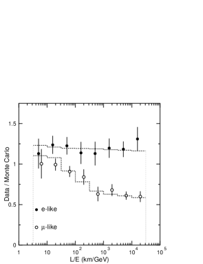
FIG. 4.: The ratio of the number of data events to Monte Carlo calculated events (in the absence of oscillations) in Super-Kamiokande, as a function of reconstructed $L/E$ [4]. The points show the ratio of observed data and Monte Carlo expectation. The dashed lines show the expected ratios for $\nu_{\mu}\to\nu_{\tau}$ (or $\nu_{\mu}\to\nu_{s}$) oscillations with $\Delta{m}^{2}=2.2\times 10^{-3}\,\mathrm{eV}^{2}$ and $\sin^{2}2\vartheta=1$. The slight $L/E$ dependence of the ratio for $e$-like events is due to contamination of $\nu_{\mu}$ CC interactions (2–7%).

The neutrino transition probabilities also depend on the parameter $L/E$. In Fig. 4 the ratio of the numbers of observed and predicted muon (electron) events as a function of $L/E$ is shown. The ratio practically does not depend on $L/E$ for the electron events, but strongly depends on $L/E$ for the muon events. In the region $L/E\gtrsim 10^{3}\mathrm{km}/\mathrm{GeV}$ the argument of the cosine in the expression for the $\nu_{\mu}$ survival probability (see Eq.(46)) is large and the cosine in the $\nu_{\mu}$ survival probability disappears due to averaging over energies and distances. As a result, in this region we have $\langle P_{\nu_{\mu}\to\nu_{\mu}}\rangle\simeq 1-\frac{1}{2}\sin^{2}{2\vartheta}\simeq\frac{1}{2}$ (see the last four points in Fig. 4). The disappearance of atmospheric muon neutrinos can also be explained by $\nu_{\mu}\to\nu_{s}$ oscillations. These two alternatives can be distinguished with the observation of atmospheric neutrinos through the NC process [51, 52]

$$\nu_{\ell}+A\to\nu_{\ell}+\pi^{0}+X\qquad(\ell=e,\mu,\tau)\,.$$ (68)

If $\nu_{\mu}$’s transform into sterile states, an up-down asymmetry of $\pi^{0}$ events should be observed. Another possibility to distinguish the $\nu_{\mu}\to\nu_{\tau}$ and $\nu_{\mu}\to\nu_{s}$ channels is to look for matter effects. The investigation of both effects allowed the Super-Kamiokande Collaboration to exclude pure $\nu_{\mu}\to\nu_{s}$ transitions at $2\sigma$ level [6, 7, 8].

The value $\Delta{m}^{2}\simeq 10^{-3}\,\mathrm{eV}^{2}$, which is just right in explaining the atmospheric neutrino data, can be probed in the long-baseline (LBL) reactor and accelerator experiments with a distance between source and detector about 1 km in the case of reactors and about 1000 km in the case of accelerators. No indications in favor of neutrino oscillations were found in the first reactor LBL experiment CHOOZ [53]. The CHOOZ data exclude transitions of $\bar{\nu}_{e}$ into all other possible antineutrinos for $\Delta{m}^{2}\gtrsim 10^{-3}\,\mathrm{eV}^{2}$ and $\sin^{2}{2\vartheta}\gtrsim 0.1$.

The first accelerator LBL experiment K2K, from KEK to Super-Kamiokande (a distance of about 250 km), started in Japan in 1999 [51]. The Fermilab–Soudan (a distance of about 730 km) LBL experiment MINOS [54] and the CERN-Gran Sasso (a distance of about 730 km) program of LBL experiments [55] will start after the year 2000. These experiments will investigate in detail the transitions of accelerator $\nu_{\mu}$ ’s into all possible states in the atmospheric neutrino region of $\Delta{m}^{2}$.

We will now discuss the results of solar neutrino experiments. The energy of the Sun is produced in the reactions of the thermonuclear $pp$ chain and CNO cycle. From the thermodynamical point of view, the source of the energy of the Sun is a transformation of four protons into ⁴He:

$$4p\to{}^{4}\mathrm{He}+2e^{+}+2\nu_{e}\,.$$ (69)

Thus, the production of the energy of the Sun is accompanied by the emission of electron neutrinos.

reaction	neutrino energy (MeV)	expected flux [56] (cm-2 s-1)
$p+p\to d+e^{+}+\nu_{e}$	$\leqslant 0.42$	$5.9\times 10^{10}$
$e^{-}+{}^{7}\mathrm{Be}\to{}^{7}\mathrm{Li}+\nu_{e}$	$0.86$	$4.8\times 10^{9}$
${}^{8}\mathrm{B}\to{}^{8}\mathrm{Be}^{*}+e^{+}+\nu_{e}$	$\lesssim 15$	$5.2\times 10^{6}$

TABLE II.: Main sources of solar $\nu_{e}$’s.

The main sources of $\nu_{e}$ are the reactions of the $pp$ chain that are listed in Table II, and the neutrinos coming from these sources are called $pp$, ⁷Be and ⁸B neutrinos, respectively. Neutrinos from other sources are called $pep$, $hep$ (from the reactions $p+e^{-}+p\to d+\nu_{e}$, ${}^{3}\mathrm{He}+p\to{}^{4}\mathrm{He}+e^{+}+\nu_{e}$ of the $pp$ chain) and ¹³N, ¹⁵O, ¹⁷F (from the reactions ${}^{13}\mathrm{N}\to{}^{13}\mathrm{C}+e^{+}+\nu_{e}$, ${}^{15}\mathrm{O}\to{}^{15}\mathrm{N}+e^{+}+\nu_{e}$, ${}^{17}\mathrm{F}\to{}^{17}\mathrm{O}+e^{+}+\nu_{e}$ of the CNO cycle) neutrinos. As one can see from Table II, the major part of solar neutrinos are low energy $pp$ neutrinos with $E\leqslant 0.42\,\mathrm{MeV}$. There are about 10% of monoenergetic ⁷Be neutrinos with an energy of 0.86 MeV, whereas the high energy ⁸B neutrinos ($E\lesssim 15\,\mathrm{MeV}$) constitute a very small part of the total flux of $\nu_{e}$’s from the Sun. However, as we will see later, these neutrinos give the major contribution to the event rates of experiments with a high threshold.

Assuming that $P_{\nu_{e}\to\nu_{e}}^{\mathrm{sun}}=1$ and that the Sun is in a stable state, the transition in Eq.(69) implies the following general relation between the neutrino fluxes and the luminosity of the Sun [28] $\mathcal{L}_{\odot}=2.40\times 10^{39}\,\mathrm{MeV}\,\mathrm{s}^{-1}$:

$$\sum_{r}\left(\frac{Q}{2}-\overline{E}_{r}\right)\Phi_{r}=\frac{{\mathcal{L}}_{\odot}}{4\pi R^{2}}\,,$$ (70)

with $r=pp,\,{}^{7}\mathrm{Be},\,{}^{8}\mathrm{B},\,pep,\,hep,\,{}^{13}\mathrm{N},\,{}^{15}\mathrm{O},\,{}^{17}\mathrm{F}$. Here $Q=26.7\,\mathrm{MeV}$ is the energy release in the transition (69), $R=1.50\times 10^{13}\,\mathrm{cm}$ is the Sun–Earth distance, and $\Phi_{r}$ and $\overline{E}_{r}$ are the total flux and the average energy of neutrinos from the source $r$, respectively.

Now let us turn to the experimental data. The pioneering Chlorine solar neutrino experiment by R. Davis et al. [13] known as the Homestake experiment started more than 30 years ago. Now the results of five solar neutrino experiments are available. These results are presented in Table III.

Homestake [13], GALLEX [15] and SAGE [16] are underground radiochemical experiments. The target in the Homestake experiment is a tank filled with 615 tons of C₂Cl₄ liquid. Solar neutrinos are detected in this experiment through the extraction of radioactive ³⁷Ar atoms produced in the Pontecorvo-Davis reaction

$$\nu_{e}+{}^{37}\mathrm{Cl}\rightarrow e^{-}+{}^{37}\mathrm{Ar}\,.$$ (71)

The atoms of ³⁷Ar are extracted from the tank by purging it with ⁴He gas and the Auger electrons produced in the capture of $e^{-}$ by ³⁷Ar are detected in a low-background proportional counter. During a typical exposure time of 2 months about 16 atoms of ³⁷Ar are extracted from the volume that contains $2.2\times 10^{30}$ atoms of ³⁷Cl!

The observed event rate in the Homestake experiment averaged over 108 runs is $2.56\pm 0.23$ SNU, whereas the event rate predicted by the Standard Solar Model (SSM) [56] is $7.7\pm 1.2$ SNU.

The threshold of the reaction (71) is $E_{\mathrm{th}}=0.81\,\mathrm{MeV}$. Thus, low energy $pp$ neutrinos cannot be detected in the Homestake experiment. The main contributions to the event rate come from ⁸B and ⁷Be neutrinos (according to the SSM, 77% and 15%, respectively).

Experiment	Observed rate	Predicted rate [56]
Homestake	$2.56\pm 0.16\pm 0.16$	$7.7\,{}^{+1.2}_{-1.0}$
GALLEX	$77.5\pm 6.2\,{}^{+4.3}_{-4.7}$	$129\,{}^{+8}_{-6}$
SAGE	$66.6\,{}^{+6.8}_{-7.1}\,{}^{+3.8}_{-4.0}$	”
Kamiokande	$(2.80\pm 0.19\pm 0.33)\times 10^{6}$	$(5.15\,{}^{+1.0}_{-0.7})\times 10^{6}$
Super-Kamiokande	$(2.45\pm 0.04\pm 0.07)\times 10^{6}$	”

TABLE III.: The results of solar neutrino experiments. The rates measured in Homestake, GALLEX and SAGE are given in SNU ($1\,\mathrm{SNU}=10^{-36}\,\mathrm{events/atom/sec}$). The rates measured in Kamiokande and Super-Kamiokande are given in $\mathrm{cm}^{-2}\mathrm{s}^{-1}$.

Neutrinos from all the reactions in the Sun are detected in the radiochemical Gallium experiments GALLEX (30.3 tons of ⁷¹Ga in gallium-chloride solution) and SAGE (57 tons of ⁷¹Ga in metallic form). The detection is based on the observation of radioactive ⁷¹Ge atoms produced in the reaction

$$\nu_{e}+{}^{71}\mathrm{Ga}\rightarrow e^{-}+{}^{71}\mathrm{Ge}\,,$$ (72)

whose threshold is $E_{\mathrm{th}}=0.23\,\mathrm{MeV}$. The event rates observed in the GALLEX and SAGE experiments are about 1/2 of the predicted rates (see Table III).

In the underground Kamiokande [14] and Super-Kamiokande [17, 8] water-Cherenkov experiments, the solar neutrinos are detected in real time through the observation of the recoil electron in the process

$$\nu+e\to\nu+e\,.$$ (73)

Most importantly, in these experiments the direction of neutrinos can be determined through the the measurement of the direction of the recoil electrons. Because of the low energy background from natural radioactivity, the thresholds in the Kamiokande and Super-Kamiokande experiments are rather high: $E_{\mathrm{th}}\simeq 7\,\mathrm{MeV}$ and $E_{\mathrm{th}}\simeq 5.5\,\mathrm{MeV}$, respectively. Thus, in these experiments only ⁸B neutrinos are detected.

The results of the Kamiokande and Super-Kamiokande experiments are presented in Table III. As it can be seen from this Table, the ⁸B neutrino flux observed in these experiments is significantly smaller (about 1/2) than the SSM prediction.

Thus, in all the solar neutrino experiments a deficit of solar $\nu_{e}$’s is observed. This deficit constitutes the solar neutrino problem. What is the origin of the problem?

The predictions of the SSM are considered as rather robust [56, 57]. The model takes into account all the existing data on nuclear cross sections, opacities, etc. and is in impressive agreement with precise helioseismological data. It is a consensus that the solar neutrino problem should be attributed to neutrino properties.

Let us first discuss some model-independent conclusions that can be inferred from the solar neutrino data. In the gallium experiments, neutrinos from all the solar sources are detected. From the luminosity constraint (70), we have the following lower bound for the event rate in the gallium experiments:

$$S_{\mathrm{Ga}}=\int\mathrm{d}E\ \sigma_{\mathrm{Ga}}(E)\sum_{r}\Phi_{r}(E)\geqslant 76\pm 2\ \mathrm{SNU}\,.$$ (74)

The data of the GALLEX and SAGE experiments are compatible with this bound (see the Table III). Thus, on the basis of the luminosity constraint alone, one cannot conclude that the solar neutrino problem exists. However, we can see that the problem exists if we compare the data obtained from different solar neutrino experiments [58, 36].

Let us assume that $P_{\nu_{e}\to\nu_{e}}^{\mathrm{sun}}=1$ and let us consider the total neutrino fluxes $\Phi_{r}$ as free variable parameters. From the data of the Super-Kamiokande experiment it follows that the flux of ⁸B neutrinos is

$$\Phi_{{}^{8}\mathrm{B}}=(2.44\pm 0.10)\times 10^{6}\,\mathrm{cm}^{-2}\,\mathrm{s}^{-1}\,.$$ (75)

If we subtract the contribution of ⁸B neutrinos from the event rate observed in the Homestake experiment, we obtain an upper bound for the contribution of ⁷Be neutrinos to the chlorine event rate:

$$S^{{}^{7}\mathrm{B}}_{\mathrm{Cl}}\leqslant S^{\mathrm{exp}}_{\mathrm{Cl}}-S^{{}^{8}\mathrm{B}}_{\mathrm{Cl}}=-0.22\pm 0.35\ \mathrm{SNU}\,.$$ (76)

According to the SSM, the contribution of ⁷Be neutrinos to the Chlorine event rate is significantly larger ($S^{{}^{7}\mathrm{B}}_{\mathrm{Cl}}(\mathrm{SSM})=1.1\pm 0.1\,\mathrm{SNU}$). Such a strong suppression of the flux of ⁷Be neutrinos cannot be explained by any known astrophysical mechanism [57]. One can reach the same conclusion using the Super-Kamiokande and GALLEX-SAGE data.

The solar neutrinos problem can be solved if we assume that the solar $\nu_{e}$’s transform into another flavor ($\nu_{\mu}$, $\nu_{\tau}$) or sterile states through neutrino oscillations. In order to explain all the existing solar neutrino data, it is sufficient to assume that transitions between two neutrino states alone take place.

The solar neutrinos produced in the thermonuclear reactions in the central zone of the Sun pass through a large amount of matter on the way to the Earth. If the value of the parameter $\Delta{m}^{2}$ lies between $\sim 10^{-8}\,\mathrm{eV}^{2}$ and $\sim 10^{-4}\,\mathrm{eV}^{2}$, coherent matter effects become important and the transition probability of solar $\nu_{e}$’s into other states can be resonantly enhanced (MSW effect [59]), even for small values of the mixing angle $\vartheta$. Assuming the validity of the SSM and that the MSW effects does indeed take place, the analysis of all the solar neutrino data leads to the following two possible sets of best-fit values of the oscillation parameters [58, 60, 8]

$$\Delta{m}^{2}\simeq 5\times 10^{-6}\,\mathrm{eV}^{2}\,,\qquad\sin^{2}{2\vartheta}\simeq 5\times 10^{-3}\,,$$ (77)

$$\Delta{m}^{2}\simeq 3.2\times 10^{-5}\,\mathrm{eV}^{2}\,,\qquad\sin^{2}{2\vartheta}\simeq 0.8\,.$$ (78)

In the case of $\nu_{e}\to\nu_{s}$ transitions only small values of the mixing angle are allowed [58, 60, 61, 8].

The existing data can also be explained if $\Delta{m}^{2}\ll 10^{-8}\,\mathrm{eV}^{2}$ and matter effects are unimportant. In this case, the $\nu_{e}$ survival probability is given by the standard two neutrino vacuum expression (see Eq.(46)). From the analysis of the data, the following best-fit values of the oscillation parameters have been found [58, 62, 8]

$$\Delta{m}^{2}\simeq 4.3\times 10^{-10}\,\mathrm{eV}^{2}\,,\qquad\sin^{2}{2\vartheta}\simeq 0.79\,.$$ (79)

This solution of the solar neutrino problem is called “vacuum oscillation solution” or “just-so vacuum solution”.

Recently a new solar neutrino experiment, SNO [63], started in Canada. In this experiment, the solar ⁸B neutrinos will be detected through the charged current (CC) process, $\nu_{e}+d\to e^{-}+p+p$, the neutral current (NC) process, $\nu+d\to\nu+n+p$, and elastic neutrino-electron scattering $\nu+e\to\nu+e$.

From the detection of the solar neutrinos via the CC process, the spectrum of $\nu_{e}$’s on the Earth can be measured and compared with the well-known ⁸B neutrino spectrum predicted by the theory of weak interactions. A comparison of the measured spectrum with the predicted one can provide us with a model-independent check on whether the solar $\nu_{e}$’s have transformed into other states in a energy-dependent way. The detection of neutrinos via the NC process can determine the total flux of all flavors, $\nu_{e}$, $\nu_{\mu}$ and $\nu_{\tau}$. The comparison of the NC and CC measurements, will provide us with another possibility to check in a model-independent way whether transitions of the solar $\nu_{e}$’s into other flavor states actually take place.

From all the analyses of the solar neutrino data it follows that the flux of medium energy ⁷Be neutrinos is strongly suppressed. A future solar neutrino experiment, Borexino [64], in which mainly ⁷Be neutrinos will be detected, can check this general conclusion obtained from the existing data.

Several other future solar neutrino experiments [65] (ICARUS, GNO, LENS, HELLAZ and others) are under planning or development. In these experiments different parts of the solar neutrino spectrum will be explored in detail.

A sensitivity to values of $\Delta{m}^{2}$ as small as $\sim 10^{-5}\,\mathrm{eV}^{2}$ will be reached in the LBL reactor experiments Kam-Land in Japan [66] and Borexino in Italy [64] (with distances between reactors and detectors of about 200 km and 800 km, respectively). These experiments will be able to check the large mixing angle MSW solution of the solar neutrino problem.

The third indication in favor of neutrino oscillations was reported by the Los Alamos neutrino experiment LSND [18, 19]. In this experiment, neutrinos were produced in decays at rest of $\pi^{+}$ ($\pi^{+}\to\mu^{+}\nu_{\mu}$) and $\mu^{+}$ ($\mu^{+}\to e^{+}\nu_{e}\bar{\nu}_{\mu}$). Thus, there are no $\bar{\nu}_{e}$’s from the source. At a distance of about 30 m from the source $\bar{\nu}_{e}$’s are searched for in the large LSND detector (about 180 tons of liquid scintillator) via the process

$$\bar{\nu}_{e}+p\to e^{+}+n\,.$$ (80)

A significant number of $\bar{\nu}_{e}$ events (22 events with an expected background of $4.6\pm 0.6$ events) has been found in the range of neutrino energy $36\,\mathrm{MeV}<E<60\,\mathrm{MeV}$ [18].

The observed events can be explained by $\bar{\nu}_{\mu}\to\bar{\nu}_{e}$ oscillations. Taking into account the results of other reactor and accelerator experiments, in which neutrino oscillations were not observed, the following ranges for the oscillation parameters are allowed:

$$0.2\,\mathrm{eV}^{2}\lesssim\Delta{m}^{2}\lesssim 2\,\mathrm{eV}^{2}\,,\qquad 3\times 10^{-3}\lesssim\sin^{2}{2\vartheta}\lesssim 4\times 10^{-2}\,.$$ (81)

The LSND Collaboration found also some evidence in favor of $\nu_{\mu}\to\nu_{e}$ transitions of the $\nu_{\mu}$’s generated by $\pi^{+}$ decay in flight [19]. The $\nu_{e}$’s produced in this way can be distinguished from the $\nu_{e}$’s generated by $\mu^{+}$ decay at rest because they have higher energies. The resulting allowed values of the parameters $\Delta{m}^{2}$ and $\sin^{2}2\vartheta$ are compatible with those in Eq.(81).

In another accelerator experiment, KARMEN [67], designed to find $\bar{\nu}_{\mu}\to\bar{\nu}_{e}$ oscillations, no positive signal was found. The sensitivity of the KARMEN experiment to the value of the parameter $\sin^{2}{2\vartheta}$ is, however, smaller than the sensitivity of the LSND experiment and at the moment there is no contradiction between the results of these two experiments, although part of the LSND allowed region is disfavored by the results of the KARMEN experiment. New experiments are needed in order to investigate in detail the LSND anomaly. Four such experiments have been proposed and are under study: BooNE [68] at Fermilab, I-216 [69] at CERN, ORLaND [70] at Oak Ridge and NESS at the European Spallation Source [71]. Among these proposals BooNE is approved and will start in the year 2001.

In summary, indications in favor of nonzero neutrino masses and neutrino mixing have been found in the atmospheric, solar and LSND neutrino experiments. What conclusions can we drawn about the possible neutrino mass spectra and the values of the elements of the neutrino mixing matrix $U$ from the data of these experiments?

Assuming the validity of the solar and atmospheric indications in favor of neutrino oscillations, the types of neutrino mass spectra allowed by the data crucially depend on the validity of the LSND result. If this result fails to be confirmed by future experiments, three massive neutrinos with the hierarchical mass spectrum of see-saw type and with $\Delta{m}^{2}_{21}$ relevant for the oscillations of solar neutrinos and $\Delta{m}^{2}_{31}$ relevant for the oscillations of atmospheric neutrinos are enough to describe all the existing data [72].

The CHOOZ and Super-Kamiokande results suggest that, in the three neutrino case, the element $|U_{e3}|^{2}$ is small [73, 74]. This means that the oscillations of solar and atmospheric neutrinos are practically decoupled and are described by the two-neutrino formalism. Neutrinos are very light in this scenario: the heaviest mass is $m_{3}\simeq 5\times 10^{-2}\mathrm{eV}^{2}$. In order to answer the fundamental question as to whether massive neutrinos are Dirac or Majorana particles, it is necessary to increase the sensitivity of the experiments searching for neutrinoless double-$\beta$ decay by at least one order of magnitude [75, 76].

If the LSND result is confirmed, at least three different scales of $\Delta{m}^{2}$ (LSND, atmospheric and solar) are needed in order to describe the data, which implies that there are at least four massive (but light) neutrinos. In the minimal scheme with four massive neutrinos, only the two mass spectra

$$\mbox{(A)}\qquad\underbrace{\overbrace{m_{1}<m_{2}}^{\mathrm{atm}}\ll\overbrace{m_{3}<m_{4}}^{\mathrm{sun}}}_{\mathrm{LSND}}\qquad\mbox{and}\qquad\mbox{(B)}\qquad\underbrace{\overbrace{m_{1}<m_{2}}^{\mathrm{sun}}\ll\overbrace{m_{3}<m_{4}}^{\mathrm{atm}}}_{\mathrm{LSND}}\,,$$ (82)

with two couples of close masses separated by the the ”LSND gap” of about 1 eV, are compatible with all the existing data [77]. The existence of four massive light neutrinos implies that a sterile neutrino should exist in addition to the flavor neutrinos $\nu_{e}$, $\nu_{\mu}$ and $\nu_{\tau}$. Furthermore, if the standard Big-Bang Nucleosynthesis constraint on the number of light neutrinos [78] is less than 4 [79], there is a stringent limit on the mixing of the sterile neutrino with the two massive neutrinos that are responsible for the oscillations of atmospheric neutrinos and the two allowed schemes have the form shown in Fig. 5 [80, 81], i.e. $\nu_{s}$ is mainly mixed with the two massive neutrinos that contribute to solar neutrino oscillations ($\nu_{3}$ and $\nu_{4}$ in scheme A and $\nu_{1}$ and $\nu_{2}$ in scheme B) and $\nu_{\tau}$ is mainly mixed with the two massive neutrinos that contribute to the oscillations of atmospheric neutrinos.

In the extended SM with massive neutrinos, there is no room for sterile neutrinos. Thus, a successful explanation of all the existing data requires new exciting physics.

FIG. 5.: The two types of neutrino mass spectra that can accommodate the solar, atmospheric and LSND scales of $\Delta{m}^{2}$ and the mixing schemes that emerge if the Big-Bang Nucleosynthesis constraint on the number of light neutrinos is less than 4.

VI Conclusions

The evidence in favor of oscillations of atmospheric neutrinos found in the Super-Kamiokande experiment and the indications in favor of oscillations obtained in other atmospheric neutrino experiments, in the solar neutrino experiments and in the LSND experiment has opened a new chapter in neutrino physics: the physics of massive and mixed neutrinos.

There are many open problems in the physics of massive neutrinos.

We are now anxiously waiting for the results of the new neutrino oscillation experiments SNO and K2K, that started their operation in 1999, and the future experiments Borexino, ICARUS, BooNe, MINOS and many others, that will start after the year 2001. We hope that the results of these experiments will answer the questions that have been puzzling us for the past decades.

There is no doubt that the program of future investigations of neutrino oscillations will lead to a significant progress in understanding the origin of the tiny neutrino masses and of neutrino mixing, which is undoubtedly of extreme importance for the future of elementary particle physics and astrophysics.

REFERENCES

- [1] S.L. Glashow, Nucl. Phys. 22, 597 (1961); S. Weinberg, Phys. Rev. Lett. 19, 1264 (1967); A. Salam, Proc. of the 8th Nobel Symposium on Elementary particle theory, relativistic groups and analyticity, edited by N. Svartholm, 1969.
- [2] S.L. Glashow, J. Iliopoulos and L. Maiani, Phys. Rev. D 2, 1285 (1970).
- [3] See, for example, J. Ellis, hep-ph/9812235, Lectures presented at 1998 European School of High-Energy Physics.
- [4] Y. Fukuda et al., Super-Kamiokande Coll., Phys. Rev. Lett. 81, 1562 (1998); Phys. Rev. Lett. 82, 2644 (1999).
- [5] K. Scholberg (Super-Kamiokande Coll.), hep-ex/9905016, Talk presented at the VIIIth International Workshop on Neutrino Telescopes, Venice, 23–26 February 1999.
- [6] T. Kajita (Super-Kamiokande Coll.), Talk presented at BEYOND’99, Castle Ringberg, Tegernsee, Germany, 6–12 June 1999.
- [7] J. Learned (Super-Kamiokande Coll.), Talk presented at the 23rd Johns Hopkins Workshop on Current Problems in Particle Theory, Neutrinos in the Next Millennium, Johns Hopkins University, Baltimore, USA, 10–12 June 1999 (transparencies available at http://www.pha.jhu.edu/events/jhwsh99/speakers.html).
- [8] M. Nakahata (Super-Kamiokande Coll.), Talk presented at TAUP’99, Paris, France, 6–10 September 1999 (transparencies available at http://taup99.in2p3.fr/TAUP99/program.html).
- [9] Y. Fukuda et al. (Kamiokande Coll.), Phys. Lett. B335, 237 (1994).
- [10] R. Becker-Szendy et al. (IMB Coll.), Nucl. Phys. B (Proc. Suppl.) 38, 331 (1995).
- [11] W.W.M. Allison et al. (Soudan2 Coll.), Phys. Lett. B 391, 491 (1997); Phys. Lett. B 449, 137 (1999); T. Kafka (Soudan2 Coll.), Talk presented at TAUP’99, Paris, France, 6–10 September 1999 (transparencies available at http://taup99.in2p3.fr/TAUP99/program.html).
- [12] M. Ambrosio et al. (MACRO Coll.), Phys. Lett. B 434, 451 (1998); M. Spurio (MACRO Coll.), hep-ex/9908066.
- [13] B.T. Cleveland et al. (Homestake Coll.), Astrophys. J. 496, 505 (1998).
- [14] K.S. Hirata et al. (Kamiokande Coll.), Phys. Rev. Lett. 77, 1683 (1996).
- [15] W. Hampel et al. (GALLEX Coll.), Phys. Lett. B447, 127 (1999).
- [16] J.N. Abdurashitov et al. (SAGE Coll.), Phys. Rev. Lett. 77, 4708 (1996); Phys. Rev. C 60, 055801 (1999).
- [17] Y. Fukuda et al. (Super-Kamiokande Coll.), Phys. Rev. Lett. 81, 1158 (1998); Phys. Rev. Lett. 82, 2430 (1999); M.B. Smy (Super-Kamiokande Coll.), hep-ex/9903034.
- [18] C. Athanassopoulos et al., LSND Coll., Phys. Rev. Lett. 77, 3082 (1996).
- [19] C. Athanassopoulos et al., LSND Coll., Phys. Rev. Lett. 81, 1774 (1998).
- [20] See, for example, F. Wilczek, Nucl. Phys. B (Proc. Suppl.) 77, 511 (1999).
- [21] C.S. Wu et al., Phys. Rev. 105, 1413 (1957).
- [22] L. Landau, Nucl. Phys. 3, 127 (1957).
- [23] T.D. Lee and C.N. Yang, Phys. Rev. 105, 1671 (1957).
- [24] A. Salam, Il Nuovo Cimento 5, 299 (1957).
- [25] M. Goldhaber, L. Grodzins and A.W. Sunyar, Phys. Rev. 109, 1015 (1958).
- [26] R.P. Feynman and M. Gell-Mann, Phys. Rev. 109, 193 (1958).
- [27] E.C.G. Sudarshan and R. Marshak, Phys. Rev. 109, 1860 (1958).
- [28] C. Caso et al., Particle Data Group, Eur. Phys. J. C 3, 1 (1998).
- [29] N. Cabibbo, Phys. Rev. Lett. 10, 531 (1963); M. Kobayashi and K. Maskawa, Prog. Theor. Phys. 49, 652 (1973).
- [30] J.H. Christenson, J.W. Cronin, V.L. Fitch and R. Turlay, Phys. Rev. Lett. 13, 138 (1964); Phys. Rev. 140, B74 (1965).
- [31] V. Lobashov, Talk presented at Neutrino ’98 [48]; C. Weinheimer, Talk presented at Neutrino ’98 [48].
- [32] K. Assamagan et al., Phys. Rev. D 53, 6065 (1996).
- [33] R. Barate et al., Eur. Phys. J. C 2, 395 (1998).
- [34] M. Gell-Mann, P. Ramond, and R. Slansky, in Supergravity, ed. F. van Nieuwenhuizen and D. Freedman (North Holland, Amsterdam, 1979), p.315; T. Yanagida, Proc. of the Workshop on Unified Theory and the Baryon Number of the Universe, KEK, Japan, 1979; R.N. Mohapatra and G. Senjanović, Phys. Rev. Lett. 44, 912 (1980).
- [35] S.M. Bilenky and B. Pontecorvo, Phys. Rep. 41, 225 (1978); S.M. Bilenky and S.T. Petcov Rev. Mod. Phys. 59, 671 (1987); R.N. Mohapatra and P.B. Pal, Massive Neutrinos in Physics and Astrophysics, World Scientific Lecture Notes in Physics, Vol.41, World Scientific, Singapore, 1991; C.W. Kim and A. Pevsner, Neutrinos in Physics and Astrophysics, Contemporary Concepts in Physics, Vol.8, Harwood Academic Press, Chur, Switzerland, 1993.
- [36] S.M. Bilenky, C. Giunti and W. Grimus, Prog. Part. Nucl. Phys. 43, 1 (1999), hep-ph/9812360.
- [37] B. Pontecorvo, J. Exptl. Theoret. Phys. 33, 549 (1957) [Sov. Phys. JETP 6, 429 (1958)]; J. Exptl. Theoret. Phys. 34, 247 (1958) [Sov. Phys. JETP 7, 172 (1958)].
- [38] Z. Maki, M. Nakagawa and S. Sakata, Prog. Theor. Phys. 28, 870 (1962).
- [39] D. Orestano (NOMAD Coll.), Talk presented at the CAPP 98 Workshop, CERN, June, 1998 (NOMAD WWW page: http://nomadinfo.cern.ch).
- [40] F. Dydak et al., CDHS Coll., Phys. Lett. B 134, 281 (1984).
- [41] N. Ushida et al., Phys. Rev. Lett. 57, 2897 (1986).
- [42] P. Vilain et al., CHARM II Coll., Z. Phys. C 64, 539 (1994).
- [43] K.S. McFarland et al., CCFR Coll., Phys. Rev. Lett. 75, 3993 (1995).
- [44] CHORUS Coll., hep-ex/9907015.
- [45] J. Altegoer et al. (NOMAD Coll.), Phys. Lett. B431, 219 (1998).
- [46] A. De Rujula et al., Nucl. Phys. B 168, 54 (1980); V. Barger and K. Whisnant, Phys. Lett. B 209, 365 (1988); S.M. Bilenky, M. Fabbrichesi and S.T. Petcov, Phys. Lett. B 276, 223 (1992).
- [47] S.M. Bilenky, A. Bottino, C. Giunti and C.W. Kim Phys. Rev. D 54, 1881 (1996); S.M. Bilenky, C. Giunti and C.W. Kim, Astrop. Phys. 4, 241 (1996); C. Giunti, C.W. Kim and M. Monteno, Nucl. Phys. B 521, 3 (1998).
- [48] International Conference on Neutrino Physics and Astrophysics Neutrino ’98, Takayama, Japan, June 1998; WWW page: http://www-sk.icrr.u-tokyo.ac.jp/nu98.
- [49] T.K. Gaisser et al., Phys. Rev. D 54, 5578 (1996); T.K. Gaisser, hep-ph/9611301, Proc. of Neutrino ’96, Helsinki, June 1996, edited by K. Enqvist et al., p. 211, World Scientific, Singapore, 1997; Nucl. Phys. B (Proc. Suppl.) 77, 133 (1999).
- [50] K.S. Hirata et al., Kamiokande Coll., Phys. Lett. B 280, 146 (1992).
- [51] Y. Suzuki, Proc. of Neutrino 96, Helsinki, June 1996, edited by K. Enqvist et. al., p. 237, World Scientific, Singapore, 1997.
- [52] F. Vissani and A.Yu. Smirnov, Phys. Lett. B 432, 376 (1998).
- [53] M. Apollonio et al. (CHOOZ Coll.), Phys. Lett. B 420, 397 (1998); Phys. Lett. B 466, 415 (1999).
- [54] D. Ayres et al., MINOS Coll., report NUMI-L-63 (1995).
- [55] P. Picchi and F. Pietropaolo, preprint hep-ph/9812222.
- [56] J.N. Bahcall, S. Basu and M.H. Pinsonneault, Phys. Lett. B 433, 1 (1998).
- [57] J.N. Bahcall, Nucl. Phys. B (Proc. Suppl.) 77, 64 (1999).
- [58] J.N. Bahcall, P.I. Krastev and A.Yu. Smirnov, Phys. Rev. D 58, 096016 (1998).
- [59] S.P. Mikheyev and A.Yu. Smirnov, Yad. Fiz. 42, 1441 (1985) [Sov. J. Nucl. Phys. 42, 913 (1985)]; Il Nuovo Cimento C 9, 17 (1986); L. Wolfenstein, Phys. Rev. D 17, 2369 (1978); ibid. 20, 2634 (1979).
- [60] Y. Fukuda et al., Super-Kamiokande Coll., Phys. Rev. Lett. 82, 1810 (1999).
- [61] M.C. Gonzalez-Garcia et al., hep-ph/9906469.
- [62] V. Barger and K. Whisnant, Phys. Lett. B456, 54 (1999).
- [63] SNO WWW page: http://www.sno.queensu.ca.
- [64] L. Oberauer, Borexino Coll., Talk presented at Neutrino ’98 [48]; Borexino WWW pages: http://almime.mi.infn.it/; http://pupgg.princeton.edu/~borexino/welcome.html.
- [65] R.E. Lanou, Nucl. Phys. B (Proc. Suppl.) 77, 55 (1999).
- [66] F. Suekane, preprint TOHOKU-HEP-97-02 (1997); A. Suzuki, Talk presented at the VIIIth International Workshop on Neutrino Telescopes, Venice, 23–26 February 1999.
- [67] T. Jannakos (KARMEN Coll.), http://www-ik1.fzk.de/www/karmen/ps/moriond99_2.ps, Talk presented at Les Rencontres De Moriond 1999, 13–20 March 1999, Les Arc 1800; M. Steidl (KARMEN Coll.) http://www-ik1.fzk.de/www/karmen/ps/thuile99.ps, Talk presented at Les Rencontres De Physique De La Vallee Aoste 1999, 28 Feb – 6 March 1999, La Thuile.
- [68] Booster Neutrino Experiment (BooNE), http://nu1.lampf.lanl.gov/BooNE.
- [69] I-216 proposal at CERN, http://chorus01.cern.ch/~pzucchel/loi/.
- [70] Oak Ridge Large Neutrino Detector, http://www.phys.subr.edu/orland/.
- [71] NESS: Neutrinos at the European Spallation Source, http://www.isis.rl.ac.uk/ess/neut%5Fess.htm.
- [72] G.L. Fogli, E. Lisi and D. Montanino Phys. Rev. D 49, 3626 (1994); Astropart. Phys. 4 177 (1995); Phys. Rev. D 54, 2048 (1996); Astropart. Phys. 9, 119 (1998); G.L. Fogli and E. Lisi and D. Montanino and G. Scioscia, Phys. Rev. D 55, 4385 (1997).
- [73] F. Vissani, preprint hep-ph/9708483.
- [74] S.M. Bilenky and C. Giunti, Phys. Lett. B 444, 379 (1998).
- [75] S.M. Bilenky, C. Giunti, C.W. Kim and M. Monteno, Phys. Rev. D 57, 6981 (1998).
- [76] S.M. Bilenky, C. Giunti, W. Grimus, B. Kayser and S.T. Petcov, Phys. Lett. B 465, 193 (1999).
- [77] S.M. Bilenky, C. Giunti and W. Grimus, Eur. Phys. J. C 1, 247 (1998); hep-ph/9609343, Proc. of Neutrino ’96, p. 174, Helsinki, June 1996, edited by K. Enqvist et al., World Scientific, Singapore, 1997; S.M. Bilenky, C. Giunti, W. Grimus and T. Schwetz, Phys. Rev. D60, 073007 (1999).
- [78] S. Sarkar, Rept. Prog. Phys. 59, 1493 (1996); D.N. Schramm and M.S. Turner, Rev. Mod. Phys. 70, 303 (1998); K.A. Olive, astro-ph/9707212; astro-ph/9712160; A.D. Dolgov, astro-ph/9807134 E. Lisi, S. Sarkar and F.L. Villante, Phys. Rev. D59, 123520 (1999); S. Sarkar, astro-ph/9903183; K.A. Olive, G. Steigman and T.P. Walker, astro-ph/9905320.
- [79] S. Burles, K.M. Nollett, J.N. Truran and M.S. Turner, Phys. Rev. Lett. 82, 4176 (1999).
- [80] N. Okada and O. Yasuda, Int. J. Mod. Phys. A 12, 3669 (1997).
- [81] S.M. Bilenky, C. Giunti, W. Grimus and T. Schwetz, Astropart. Phys. 11, 413 (1999).