Stronger constraints for nanometer scale Yukawa-type hypothetical interactions from
the new measurement of the Casimir force

Abstract

We consider the Casimir force including all important corrections to it for the configuration used in a recent experiment employing an atomic force microscope. We calculate the long-range hypothetical forces due to the exchange of light and massless elementary particles between the atoms constituting the bodies used in the experiment — a dielectric plate and a sphere both covered by two thin metallic layers. The corrections to these forces caused by the small surface distortions were found to be essential for nanometer Compton wave lengthes of hypothetical particles. New constraints for the constants of Yukawa-type interactions are obtained from the fact that such interactions were not observed within the limits of experimental accuracy. They are stronger up to 140 times in some range than the best constraints known up date. Different possibilities are also discussed to strengthen the obtained constraints in several times without principal changes of the experimental setup.

I INTRODUCTION

Hypothetical interactions of Yukawa- and power-types have been discussed actively in recent years (for a collection of references on this subject, see [1]). They may be considered as specific corrections to the classical gravitational force at small distances [2]. An alternative interpretation comes from the elementary particle physics. According to the unified gauge theories, supersymmetry and supergravity [3], there would exist a number of light or massless elementary particles (for example, axion, scalar axion, graviphoton, dilaton, arion, and others). The exchange of such particles between two atoms gives rise to an interatomic force described by Yukawa or power-law effective potentials. The interaction range of this force is to be considered from one angström to hundreds of kilometers. Because of this, it is called a “long-range force” (in comparison with the nuclear size).

The constraints for the constants of these hypothetical long-range interactions lead to new knowledge about the parameters of associated elementary particles. Such constraints are obtainable from Galileo-, Eötvös- and Cavendish-type experiments, from the measurements of the van der Waals and Casimir force, transition probabilities in exotic atoms, etc [4]. The pioneering studies in the application of the Casimir force measurements to the problem of long-range interactions were made in Refs. [5–7]. There it was shown that the Casimir effect leads to the strongest constraints on the constants of Yukawa-type interactions with a range of action of $10^{-8}{\,\mbox{\rm m}}\,<\lambda<10^{-4}{\,\mbox{\rm m}}$ [4,5,7].

In the beginning of 1997 the results on the demonstration of the Casimir force between the metallized surfaces of a flat disc and a spherical lens were published [8]. The absolute error of the force measurements was $\Delta F\approx 10^{-11}\,$N for distances between the disc and the lens from one to six micrometers. This corresponds to the relative error of approximately 5% at the smallest surface separation. Some tentative conclusions from experimental observations of [8] were made in [9,10] concerning the possible constraints on long-range interactions. The detailed and accurate analyses of constraints following from [8] was given in [11] for both Yukawa- and power-type interactions with account of all different corrections to the Casimir force. It was established that the constraints for Yukawa-type interactions following from [8] are the best ones within a range $2.2\times 10^{-7}{\,\mbox{\rm m}}\leq\lambda\leq 1.6\times 10^{-4}{\,\mbox{\rm m}}$. The fact was emphasized that they surpass the previously known constraints in this range up to factor of 30.

Recently, the results of a new experiment were published [12] on the precision measurement of the Casimir force between a metallized sphere and a flat plate. The force was measured using an atomic force microscope for the plate-sphere separations from 120 nm to 900 nm. In [12] the corrections to the Casimir force were taken into account due to the finite conductivity of the metal and due to the small surface distortions (the temperature corrections are negligible in the range of the measurement). The theoretical value of the Casimir force including corrections was confirmed experimentally with the root mean square deviation $\sigma=1.6\times 10^{-12}\,$N. This gives the possibility to use the experiment [12] for obtaining much stronger constraints on the hypothetical long-range interactions at the nanometer scale.

In this paper we calculate the hypothetical forces which might appear between a sphere and a flat plate. It is shown that the surface distortions contribute to the value of the hypothetical force essentially at the nanometer scale and influence the strength of the resulting constraints. As indicated below, the experiment [12] imposes the strongest constraints for Yukawa hypothetical interactions within a range $5.9\,$nm$\leq\lambda\leq 100\,$nm. They are stronger than the previously known constraints in this range up to a factor of 140. We notice that both recent experiments on Casimir force measuring [8,12] lead to stronger constraints for Yukawa-type hypothetical interactions, and yet these constraints hold for different $\lambda$-ranges which do not intersect each other.

The paper is organized as follows. In Sec. II the necessary details of the experiment [12] are summarized and the theoretical results for the Casimir force with all the necessary corrections are discussed. Section III is devoted to the calculation of the hypothetical forces in the experimental configuration of [12]. Both the layer structure of the test bodies and small surface distortions are taken into account. Section IV contains the derivation of the new constraints for the parameters of Yukawa-type hypothetical interactions following from the experiment [12]. The possible improvement of the experimental scheme is also discussed in order to provide stronger constraints. Section V contains the conclusions and discussions.

II THE CASIMIR FORCE BETWEEN A SPHERE AND A DISC

In the experiment [12] the Casimir force was measured between a metallized polystyrene sphere of radius $R=98{\,\mu{\mbox{\rm m}}}$ and a sapphire disc of diameter $D=1.25\,$cm (see Fig. 1). The sphere was attached to a cantilever of an atomic force microscope. The sphere and the disc were covered by a layer of $Al$ with $\Delta_{1}^{\prime}=\Delta_{1}=300\,$nm thickness. Both surfaces were covered then by a layer of $60\%Au/40\%Pd$ with $\Delta_{2}^{\prime}=\Delta_{2}=20\,$nm (the thicknesses in Fig 1 are shown to be different on both bodies for generality). Disc-sphere surface separations lie in the range $120\,$nm$\leq\lambda\leq 900\,$nm.

The Casimir force in the configuration of Fig. 1 is the same as in the configuration of a spherical lens above an infinite disc due to inequalities $a\ll R\ll D$:

$$F^{(0)}(a)=-\frac{\pi^{3}}{360}\,R\,\frac{\hbar c}{a^{3}}.$$ (1)

This formula was derived in [13] for the first time and reobtained by different authors afterwards (see, e.g., [14–16]).

In the range of $a$ under consideration the substantial corrections to Eq. (1) are due to the finite conductivity of the metal and due to the surface distortions (the temperature corrections are important for larger surface separations [11]). The corrections due to the finite conductivity can be obtained by the use of perturbation theory in the small parameter $\delta_{0}/a=c/(\omega_{p}a)=\lambda_{p}/(2\pi a)$, where $\omega_{p}(\lambda_{p})$ is the effective plasma frequency (wave-length) of the electrons, $\delta_{0}$ is the penetration depth of the electromagnetic oscillations into the metal. For $Al$ we have $\lambda_{p}\approx 100\,$nm [12] (the external metallic layer is rather transparent, so it is equivalent to several nanometers of $Al$ only). Thus, the value of $\delta_{0}/a$ changes from 0.133 to 0.018 in the range of the measurement.

The first order correction to (1) was firstly found in [17] for the configuration of two plane parallel plates (see also [18]). The second order correction was obtained in [19]. We finally obtain for the case of plane parallel plates

$$F_{\delta_{0}}(a)\approx F^{(0)}(a)\left(1-\frac{16}{3}\,\frac{\delta_{0}}{a}+24\,\frac{\delta_{0}^{2}}{a^{2}}\right).$$ (2)

From the exact expression of $F_{\delta_{0}}$ (before the expansion in powers of $\delta_{0}/a$) it is quite clear that $F_{\delta_{0}}$ is sign-constant for all $\delta_{0}$ and tends to zero in the formal limit $\delta_{0}\to\infty$. This allows us to obtain a simple interpolation formula. It gives the same result as (2) for small $\delta_{0}/a$, but applicable over a broader interval $0\leq\delta_{0}/a\,{\scriptscriptstyle{\stackrel{{\scriptstyle<}}{{\sim}}}}\,0.2$ [14]

$$F_{\delta_{0}}(a)\approx F^{(0)}(a)\left(1+\frac{11}{3}\,\frac{\delta_{0}}{a}\right)^{-16/11}.$$ (3)

It is an easy matter to expand (3) in powers of $\delta_{0}/a$ and to modify the result to the case of a sphere above a disc by the use of the force proximity theorem [15]. The result up to fourth order is

$$F_{\delta_{0}}(a)\equiv F^{(0)}(a)+\Delta_{\delta_{0}}F^{(0)}(a)\approx F^{(0)}(a)\left(1-4\,\frac{\delta_{0}}{a}+\frac{72}{5}\,\frac{\delta_{0}^{2}}{a^{2}}-\frac{152}{3}\,\frac{\delta_{0}^{3}}{a^{3}}+\frac{532}{3}\,\frac{\delta_{0}^{4}}{a^{4}}\right).$$ (4)

Let us now discuss the corrections to (1) due to surface distortions. The character of distortions was investigated in [12] using an atomic force microscope. They look like some crystal boxes on both surfaces with a mean height $h=35\,$nm. These boxes are spaced rather rarely in a stochastic way, so that the ratio of the occupied surface area to the free one is $\beta\approx 0.11$ (see [20] for the detailed investigation of the surface distortions in [12] and their contribution to the Casimir force). The general form of the corrections to Eq. (1) due to distortions was obtained in [21] by the use of perturbation theory in the small parameters $A_{1}/a$, $A_{2}/a$. Here $A_{1,2}$ are the distortion amplitudes on both test bodies. They are defined in such a way that the mean values of the distortion functions $A_{i}f_{i}(x_{i},y_{i})$ of the first and the second body are equal to zero, and $\max|f_{i}|=1$. For two plane parallel plates the result up to the fourth order inclusive is [21]

$$F_{d}(a)\equiv F^{(0)}(a)+\Delta_{d}F^{(0)}(a)\approx F^{(0)}(a)\left[1+c_{pp}^{(1)}\left(\langle f_{1}^{2}\rangle\frac{A_{1}^{2}}{a^{2}}-2\langle f_{1}f_{2}\rangle\frac{A_{1}A_{2}}{a^{2}}+\langle f_{2}^{2}\rangle\frac{A_{2}^{2}}{a^{2}}\right)\right.$$ (5)

$$\phantom{aaaaaaa}+c_{pp}^{(2)}\left(\langle f_{1}^{3}\rangle\frac{A_{1}^{3}}{a^{3}}-3\langle f_{1}^{2}f_{2}\rangle\frac{A_{1}^{2}A_{2}}{a^{3}}+3\langle f_{1}f_{2}^{2}\rangle\frac{A_{1}A_{2}^{2}}{a^{3}}-\langle f_{2}^{3}\rangle\frac{A_{2}^{3}}{a^{3}}\right)$$ (6)

$$\phantom{aaaaaaaaaa}\left.+c_{pp}^{(3)}\left(\langle f_{1}^{4}\rangle\frac{A_{1}^{4}}{a^{4}}-4\langle f_{1}^{3}f_{2}\rangle\frac{A_{1}^{3}A_{2}}{a^{4}}+6\langle f_{1}^{2}f_{2}^{2}\rangle\frac{A_{1}^{2}A_{2}^{2}}{a^{4}}-4\langle f_{1}f_{2}^{3}\rangle\frac{A_{1}A_{2}^{3}}{a^{4}}+\langle f_{2}^{4}\rangle\frac{A_{2}^{4}}{a^{4}}\right)\right].$$ (7)

Here the angle brackets denote the averaging procedure over the area of the plates and the coefficients are $c_{pp}^{(1)}=10$, $c_{pp}^{(2)}=20$, $c_{pp}^{(3)}=35$.

The result (6) may be modified for a configuration of a sphere above a disc by the use of the force proximity theorem [15] which works good in the case of stochastic distortions [22] (as was noticed in [22] for the case of large-scale deviations on the boundary surfaces from the perfect shape the appropriate redefinition of the distance between the interacting bodies is necessary for the correct application of this theorem). Again, it has the form of (6) where the numerical coefficients $c_{pp}^{(i)}$ should be changed for $c_{ps}^{(1)}=6$, $c_{ps}^{(2)}=10$, $c_{ps}^{(3)}=15$.

For the experiment [12] $A_{1}=A_{2}=h/(1+\beta)\approx 31.5\,$nm, so that the expansion parameter in (6) changes from 0.26 to 0.035 (note that, contrary to (4), the expansion (6) starts from the second-order term). The minimal distance between the tops of two distortions situated against each other is equal to 50 nm. It is still in the action range of the Casimir forces. The quantities of the form $\langle f_{1}^{i}f_{2}^{k}\rangle$ depend on the phase shifts $\varphi_{x},\varphi_{y}$ between the distortions situated on different bodies. The measured Casimir force was averaged in [12] over 26 scans. Because of this it is necessary to consider the quantity $\langle\Delta_{d}F^{(0)}(a)\rangle_{\varphi_{x},\varphi_{y}}$ averaged over the possible values of phase shifts [20]. With a required accuracy we can use the sum of corrections to (1) due to finite conductivity and surface distortions. As a consequence of Eqs. (4), (6), the theoretical value of the Casimir force is:

$$F(a)=F^{(0)}+\Delta_{\delta_{0}}F^{(0)}(a)+\langle\Delta_{d}F^{(0)}(a)\rangle_{\varphi_{x},\varphi_{y}}.$$ (8)

As it was shown in [12, 20], the deviation of the theoretical value (8) from the experimental results is less than the absolute error of force measurements $\Delta F$ within the most interesting range 120 nm$\leq a\leq 300\,$nm (note, that in [12] there was approximately $\Delta F\approx 2\times 10^{-12}\,$N [20]). This fact is used in Sec. IV for obtaining stronger constraints for hypothetical long-range interactions.

III CALCULATION OF THE HYPOTHETICAL FORCES

As noted above, for the experimental configuration of [12] the disc can be considered as of infinite diameter. Let us start with Yukawa-type hypothetical interactions and calculate firstly the force, acting between a homogeneous disc and a sphere. The potential between two atoms which are separated by a distance $r_{12}$ and belonging to different bodies is

$$V_{Yu}=-\alpha N_{1}N_{2}\hbar c\frac{1}{r_{12}}e^{-r_{12}/\lambda},$$ (9)

where $\alpha$ is a dimensionless constant, $\lambda=\hbar/(mc)$ is the Compton wavelength of some hypothetical particle giving rise to new interaction, $N_{i}$ are the numbers of nucleons in the atomic nuclei. They are introduced into (9) to take off the dependence of $\alpha$ on the sort of atoms [23].

The potential energy of a sphere above a disc (plate) is given by

$$U_{Yu}^{(sp)}(a)=-\alpha N_{1}N_{2}\hbar c\int\limits_{V_{s}}d^{3}r_{1}\int\limits_{V_{p}}d^{3}r_{2}\frac{1}{r_{12}}e^{-r_{12}/\lambda}.$$ (10)

For the wavelength $\lambda$ at nanometer scale the plate may be considered not only as of infinite area but as of infinite width also. Integrating in (10) over $V_{p}$ one obtains

$$U_{Yu}^{(sp)}(a)=-2\pi\alpha N_{1}N_{2}\lambda^{2}\hbar c\int\limits_{V_{s}}d^{3}r_{1}e^{-z_{1}/\lambda}.$$ (11)

Here the $(x,y)$-plane of the coordinate system coincides with the surface of the plate and the $z$-axis is perpendicular to it (see Fig. 1).

Integrating over $x_{1},y_{1}$ in (11) and calculating the force as derivative

$$F_{Yu}^{(sp)}(a)=-\frac{\partial U_{Yu}^{(sp)}(a)}{\partial a},$$ (12)

we come to the expression

$$F_{Yu}^{(sp)}(a)=-2\pi^{2}\alpha N_{1}N_{2}\lambda\hbar c\int\limits_{a}^{a+2R}dz_{1}\left[R^{2}-(z_{1}-a-R)^{2}\right]e^{-z_{1}/\lambda}.$$ (13)

After the integration over $z_{1}$ the result is

$$F_{Yu}^{(sp)}(a)=-4\pi^{2}\alpha N_{1}N_{2}\lambda^{3}\hbar ce^{-a/\lambda}\,\Phi(R,\lambda),$$ (14)

where the notation

$$\Phi(R,\lambda)=R-\lambda+(R+\lambda)\,e^{-2R/\lambda}$$ (15)

is introduced.

Eq. (14) may be rewritten in terms of the densities of the sphere and the disc, respectively, $\rho^{\prime}=1.06\times 10^{3}\,$kg/m³, $\rho=4.0\times 10^{3}\,$kg/m³

$$F_{Yu}^{(sp)}(a)=-4\pi^{2}\alpha\frac{\hbar c}{m_{p}^{2}}\lambda^{3}e^{-a/\lambda}\,\Phi(R,\lambda),$$ (16)

where $m_{p}$ is the proton mass.

Using (16) it is an easy task to calculate the force acting in the configuration of the experiment [12] (see Fig. 1), i.e., taking into account the metallic layers on the sphere and the disc. For this purpose the contribution of, e.g., a layer on the sphere, may be represented as the difference of two quantities, given by (16), with the appropriate densities, radii and distances to the disc. The complete force acting in the configuration of Fig. 1 consists of twenty five contributions of the form of (16). After some rearrangements the result is

$$F_{Yu}(a)=-4\pi^{2}\alpha\frac{\hbar c}{m_{p}^{2}}\rho\rho^{\prime}\lambda^{3}e^{-\frac{a}{\lambda}}\,\left[\rho_{2}-(\rho_{2}-\rho_{1})e^{-\frac{\Delta_{2}}{\lambda}}-(\rho_{1}-\rho)e^{-\frac{\Delta_{2}+\Delta_{1}}{\lambda}}\right]$$ (17)

$$\phantom{aaaaaa}\times\left[\rho_{2}^{\prime}\Phi(R,\lambda)-(\rho_{2}^{\prime}-\rho_{1}^{\prime})\Phi(R_{1},\lambda)e^{-\frac{\Delta_{2}^{\prime}}{\lambda}}-(\rho_{1}^{\prime}-\rho^{\prime})\Phi(R_{2},\lambda)e^{-\frac{\Delta_{2}^{\prime}+\Delta_{1}^{\prime}}{\lambda}}\right].$$ (18)

Here $\rho_{2}^{\prime},\,\rho_{2}$ are the densities of the external layers on the sphere and the disc, and $\rho_{1}^{\prime},\,\rho_{1}$ are the internal ones. Also the following notations are introduced: $R_{1}=R-\Delta_{2}^{\prime}$, $R_{2}=R-\Delta_{1}^{\prime}-\Delta_{2}^{\prime}$.

One may hope to get strong constraints on $\alpha$ within the range $\lambda\sim a$ only. With regard to $a\ll R$ it follows $\lambda\ll R$ and $\Phi(R,\lambda)\approx R$ for nanometer scale of $\lambda$ we are concerned with. The result (17) may be simplified additionally when it is also taken into account that in the experiment [12] $\rho_{1}^{\prime}=\rho_{1}=2.7\times 10^{3}\,$kg/m³ and $\rho_{2}^{\prime}=\rho_{2}=16.2\times 10^{3}\,$kg/m³

$$F_{Yu}(a)=-4\pi^{2}\alpha\frac{\hbar c}{m_{p}^{2}}\lambda^{3}e^{-\frac{a}{\lambda}}\,R$$ (19)

$$\phantom{aaa}\times\left[\rho_{2}-(\rho_{2}-\rho_{1})e^{-\frac{\Delta_{2}}{\lambda}}-(\rho_{1}-\rho)e^{-\frac{\Delta_{2}+\Delta_{1}}{\lambda}}\right]\times\left[\rho_{2}-(\rho_{2}-\rho_{1})e^{-\frac{\Delta_{2}}{\lambda}}-(\rho_{1}-\rho^{\prime})e^{-\frac{\Delta_{2}+\Delta_{1}}{\lambda}}\right].$$ (20)

Now let us consider the Yukawa-type hypothetical force taking into account the surface distortions covering both the sphere and the disc. One might expect that their contribution is of prime importance when $\lambda$ is of the same order as the distortions amplitude $A$ or even smaller. The vertical distance between the distorted disc and lens surfaces is given by

$$a_{d}=a-A\left[f(x+\varphi_{x},y+\varphi_{y})+f(x,y)\right].$$ (21)

Here $f(x,y)$ is a function describing box-type distortions which are the same for both bodies, $\varphi_{x,y}$ are the phase shifts of the distortions in $x$- and $y$-coordinates between different surfaces. They may take the values from zero till the corresponding size of the characteristic distortion cell of some area $S$. Inside of this cell the quantity $a_{d}$ from (21) can have the following values

$$a_{d}=\left\{\begin{array}[]{rl}a-2A,&for\ x,y\in S_{1},\\ a-(1-\beta)A,&for\ x,y\in S_{2},\\ a+2\beta A,&for\ x,y\in S_{3},\end{array}\right.$$ (22)

when, correspondingly, there are two boxes against each other on both surfaces, a box against a nondistorted point or two nondistorted points against each other. (We remind that the parameter $\beta$ characterizing the area, occupied by distortions, was introduced in Sec. II.) Each of the values of $a_{d}$ from (22) is taken with a probability $w_{i}=S_{i}/S$; $S\equiv S_{1}\cup S_{2}\cup S_{3}$.

Clearly the areas $S_{i}$, and, consequently, the probabilities $w_{i}$, depend on $\varphi_{x}$, $\varphi_{y}$. Averaging over all the values of $\varphi_{x}$, $\varphi_{y}$, we get the averaged probabilities

$$\langle w_{1}\rangle_{\varphi_{x},\varphi_{y}}=\frac{\beta^{2}}{(1+\beta)^{2}},\quad\langle w_{2}\rangle_{\varphi_{x},\varphi_{y}}=\frac{2\beta}{(1+\beta)^{2}},\quad\langle w_{3}\rangle_{\varphi_{x},\varphi_{y}}=\frac{1}{(1+\beta)^{2}}.$$ (23)

Then the force between the distorted surfaces may be represented as a linear combination of the expressions (19) with the weights (23)

$$F_{Yu}^{(d)}(a)=\frac{2\beta}{(1+\beta)^{2}}F_{Yu}\left(a-(1-\beta)A\right)+\frac{\beta^{2}}{(1+\beta)^{2}}F_{Yu}(a-2A)+\frac{1}{(1+\beta)^{2}}F_{Yu}(a+2\beta A).$$ (24)

Substituting (19) into Eq. (24) we obtain the final result for the Yukawa-type hypothetical interaction by accounting of distortions

$$F_{Yu}^{(d)}(a)=\frac{F_{Yu}(a)}{(1+\beta)^{2}}\left[\beta^{2}e^{\frac{2A}{\lambda}}+2\beta e^{\frac{(1-\beta)A}{\lambda}}+e^{-\frac{2\beta A}{\lambda}}\right].$$ (25)

It is seen from (25) that for $\lambda\gg A$ the contribution of distortions is negligible. Expanding (25) in powers of $A/\lambda$ we find that the first nonzero correction is of second order

$$F_{Yu}^{(d)}(a)\approx F_{Yu}(a)\left(1+\beta^{2}\frac{A^{2}}{\lambda^{2}}\right).$$ (26)

So, the distortions begin to contribute when $\lambda\,{\scriptscriptstyle{\stackrel{{\scriptstyle<}}{{\sim}}}}\,80\,$nm. At $\lambda\sim 15\,$nm they determine the hypothetical force value. Here the Eq. (25) should be used in computations.

The interatomic interaction due to the exchange of massless hypothetical particles may be described by the power-law effective potentials

$$V_{n}=-\lambda_{n}N_{1}N_{2}\hbar c\frac{1}{r_{12}}\left(\frac{r_{0}}{r_{12}}\right)^{n-1},$$ (27)

where $\lambda_{n}$ are the interaction constants. The quantity $r_{0}=1\,$F$=10^{-15}{\,\mbox{\rm m}}$ is introduced to provide the proper dimensionality with different $n$ [23].

For the force between a homogeneous sphere and an infinite plate one obtains with $n\geq 3$

$$F_{n}^{(sp)}(a)=-2\pi\lambda_{n}\frac{\hbar c}{m_{p}^{2}(n-2)}\rho\rho^{\prime}r_{0}^{n-1}\int\limits_{V_{s}}d^{3}r_{1}\frac{1}{z_{1}^{n-2}}.$$ (28)

These quantities depend on $a$ very slowly. For example, integration in (28) for $n=4$ leads to the result

$$F_{4}^{(sp)}(a)=-2\pi^{2}\lambda_{4}\frac{\hbar c}{m_{p}^{2}}\rho\rho^{\prime}r_{0}^{3}\left[(R+a)\ln\frac{2R+a}{a}-2R\right].$$ (29)

Combining the appropriate number of expressions (28), (29) it is not difficult to obtain the power-type hypothetical force with account of metallic layers covering the sphere and the plate. It is evident from below, however, that the experiment [12] does not lead to any interesting new constraints for the power-type interactions. For this conclusion the expressions (28), (29) would be ample.

IV OBTAINING OF CONSTRAINTS FOR HYPOTHETICAL YUKAWA-TYPE INTERACTIONS

As it was noted in Sec. II, the theoretical expression for the Casimir force (8) was confirmed experimentally in [12,20] with the absolute error $\Delta F=2\times 10^{-12}\,$N. This means that the probable hypothetical force (if any) should be constrained by the inequality

$$|F^{hyp}(a)|\leq\Delta F=2\times 10^{-12}\,\mbox{N}.$$ (30)

Here the Yukawa-type force (19), (25) or the power-law ones (28) or (29) can play the role of $F^{hyp}(a)$.

The strongest constraints on the parameters of hypothetical interactions follow from (30) for the smallest possible value of $a=120\,$nm. Substituting (19) and (25) into (30) with account of numerical values of all involved quantities (see Secs. II, III) we obtain constraints on the Yukawa-type interaction following from the experiment [12]. They are shown by the curve 1b in Fig. 2. The region below each curve in the ($\lambda,\alpha$)-plane is permitted by the inequality (30) and above the curve it is prohibited. The curve 1a in Fig. 2 indicates constraints on Yukawa-type interaction which would be obtained without taking into account the contribution of surface distortions. In this case the total hypothetical force is given by Eq. (19) only. In the same figure curves 2 and 3 correspondingly show constraints following from the old measurements of the Casimir force [4, 7, 13, 24] and of the van der Waals force [4, 25, 26] between dielectrics. The constraints given by the curves 2, 3 were the best ones in nanometer range up to date.

It is seen that with account of surface distortions the experiment [12] leads to the best constraints for Yukawa-type interaction with a wide range of action 5.9 nm$\leq\lambda\leq$100 nm. The maximal strengthening of 140 times takes place around $\lambda=14\,$nm. Note that when neglecting the distortion contributions to the Yukawa force this range would be more narrow 8.7 nm$\leq\lambda\leq$100 nm. In this case the maximal strengthening of constraints would be about 65 times only. It is seen from Fig. 2 that the distortions cease to contribute to the strength of constraints for $\lambda\geq 25\,$nm. The $\lambda$-range in which the constraints are strengthened in ten times or more is 8.3 nm$\leq\lambda\leq$32 nm with account of distortions. This range would be more narrow (11 nm$\leq\lambda\leq$32 nm) if the distortions are neglected. By this it follows that the surface distortions contribute essentially for the Yukawa-type hypothetical force in the nanometer range and should be taken into account in all computations of constraints.

Now let us turn to the power-type hypothetical interactions. Substituting, e.g., (29) into inequality (30) one gets the constraint $\lambda_{4}\leq 3$. This result is about one thousand times weaker than the constraint obtained from the old Casimir force measurements [6]. For the power-law interactions with smaller $n$ the results are even worse. The reason is that the power-type forces between a plate and a sphere are almost independent on the distance. So, the decrease of distance in [12] in comparison to the previous experiments does not lead to an increase of the force. Meanwhile, decreasing the radius of the sphere by one thousand times (from 10 cm previously to 100$\,\mu$m now) leads to the corresponding decreasing of the hypothetical force.

The constraints, following from the experiment [12], can be strengthened additionally by a minor modification of experimental setup. Let us start with a discussion of the metallic layers covering the disc and the sphere. It is easily seen that the contribution of their interaction to hypothetical force determines its value almost completely. Actually, the contribution of a layer on a sphere and a layer on a disc is given by the combination of four expressions of the form of (16) with appropriate parameters. For example, the force acting between two outer layers is

$$F_{Yu}^{(2,2)}(a)=-4\pi^{2}\alpha\frac{\hbar c}{m_{p}^{2}}\lambda^{3}e^{-a/\lambda}\,R\rho_{2}^{2}\left(1-e^{-\Delta_{2}/\lambda}\right).$$ (31)

Performing the computations for the layers $Au/Pd$ between theirselves we come to the conclusion that they contribute 98% of the hypothetical force value at $\lambda=6\,$nm and 33% at $\lambda=100\,$nm. In the same way the contribution of $Au/Pd-Al$ layers of both bodies is 10% for $\lambda=15\,$nm and 46% for $\lambda=100\,$nm. Finally $Al-Al$ layers contribute only 1.5% of force at $\lambda=25\,$nm and 17% at $\lambda=100\,$nm. For comparison, the interaction of the sphere layers with the sapphire disc contribute only 1% of the hypothetical force at $\lambda=70\,$nm and 4% at $\lambda=100\,$nm. The interaction of the disc metallic layers with the polystyrene sphere does not contribute to the hypothetical interaction with the required accuracy not to speak of the interaction of polysterene with sapphire.

As is seen from above the main contribution to the nanometer scale Yukawa interaction is given by the $Au/Pb$ outer layers. If to change them for more heavy purely $Au$ layers of the same thickness the obtained constraints would be strengthened in 1.2 times in the range $\lambda\leq 60\,$nm. Also, the application range of new constraints would be a bit wider on the account of small $\lambda$.

The other possibility is to increase the thickness of $Au/Pb$ layer till, e.g., 25 nm (a further increasing would decrease partly the advantage of the good reflectivity properties of Al). This also gives the possibility to strengthen constraints for Yukawa interaction in 1.2 times in the range $\lambda\leq 40\,$nm.

If to combine both suggestions, i.e., to use purely $Au$ layers of 25 nm thickness, the obtained constraints would be in 1.4 times stronger.

More radical strengthening can be obtained by the use of a larger sphere. Due to the linear dependence of the hypothetical force (19) on a sphere radius $R$ the increasing of it in, e.g., 3 times would lead to the same strengthening of constraints (in this case metallic layers should cover only the top of the sphere, nearest to a disc, not to make the sphere too heavy; also a semisphere may be used with the same success). It seems to be possible also to decrease the absolute error of force measurements in 2 times, i.e., till $10^{-12}\,$N. This would strengthen constraints in 2 times simultaneously.

As a result of all these suggestions the obtained constraints could be strengthened in 8.4 times without any principal change of the setup. The maximal strengthening of the known up date constraints for Yukawa-type interaction in nanometer scale would be about 1200 times.

V CONCLUSION AND DISCUSSION

As is seen from above the new measurement of the Casimir force using an atomic force microscope gives the possibility to strengthen constraints for hypothetical Yukawa-type interaction in nanometer scale. The strengthening takes place in the range 5.9 nm$\leq\lambda\leq$100 nm. The maximal strengthening in 140 times occurs around $\lambda=$14 nm. It is interesting to compare this result with the constraints for Yukawa interaction following from the other recent experiment on measuring of the Casimir force [8]. According to the results of Ref. [11], where these constraints were obtained, the strengthening takes place in the range 220 nm$\leq\lambda\leq 1.6\times 10^{5}\,$nm. The new constraints surpass the old ones following from the measurements of the Casimir force between dielectrics up to a factor of 30. Thus, both recent experiments give complementary results which are valid in different regions. At the same time there is a wide gap for 100 nm$<\lambda<220$ nm where the former constraints are valid [4,7] obtained from the Casimir force measurements between dielectrics [13,24]. It should be covered by future experiments on measuring the Casimir force (see, e.g., a proposal to measure the Casimir force using the suspended Michelson interferometer developed for gravitational waves detection [27]).

There is a tendency of widening the range of $\lambda$ for which the Casimir effect leads to the strongest constraints on Yukawa hypothetical interactions. According to [4,7] the former measurements of the Casimir force were the source of strongest constraints in the range $10^{-8}{\,\mbox{\rm m}}\leq\lambda\leq 10^{-4}{\,\mbox{\rm m}}$. At present, combining the results following from the experiments [8,12], we get the strongest constraints in a wider range $5.9\times 10^{-9}{\,\mbox{\rm m}}\leq\lambda\leq 1.6\times 10^{-4}{\,\mbox{\rm m}}$. This means that the Casimir effect not only succeeded in obtaining stronger constraints for hypothetical interaction but also successfully compets with the measurements of van der Waals forces (in $\lambda<10^{-8}{\,\mbox{\rm m}}$ range) and with Cavendish-type experiments (for $\lambda>10^{-4}{\,\mbox{\rm m}}$). In this sense the experiments on the Casimir force measuring suggest a good supplement to the other experimental investigations giving stronger constraints for the hypothetical interactions (see, e.g., [28] where the new constraints were obtained for $\lambda\approx 0.5{\,\mbox{\rm m}}$ from the short-range test of equivalence principle or [29] where the strengthening for extremely large $\lambda$ was achieved from the satellite measurement of the Earth’s magnetic field).

As it was discussed in the preceeding section the constraints, obtained in this paper, could be strengthened by a factor of about 8 due to some modifications of experimental setup. As a result the maximal strengthening in nanometer scale may achieve of about 1000 times. According to the results of Ref. [11] the other experiment [8] on the Casimir force measuring also could lead to much stronger constraints being modified in appropriate way. This would give the possibility to constrain masses of such hypothetical elementary particles as graviphoton and dilaton by the use of the Casimir force measurements (see Ref. [30] which contains some experimental evidence for the existence of graviphoton obtained from geophysical data).

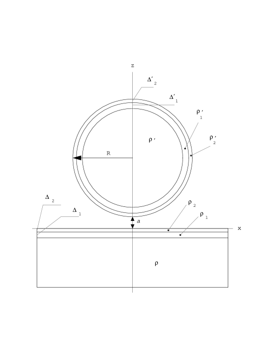
FIG. 1.: Configuration of a sphere of radius $R$ and density $\rho^{\prime}$ above a disc of density $\rho$ spaced at a distance $a$. The thicknesses and densities of $Al$ and $Au/Pd$ layers on the disc are $\Delta_{1},\,\Delta_{2},$ $\rho_{1},\,\rho_{2}$ and on the sphere are $\Delta_{1}^{\prime},\,\Delta_{2}^{\prime},$ $\rho_{1}^{\prime},\,\rho_{2}^{\prime}$, respectively.

FIG. 2.: Constraints for the constants of hypothetical Yukawa-type interactions following from different experiments. Curves 1a, 1b are obtained in this paper. They follow from the new measurement of the Casimir force [12] using an atomic force microscope (a — without account of surface distortions, b - with account of distortions). Curve 2 follows from the measurement of the Casimir force between dielectrics [4,7,13,24], curve 3 results from the van der Waals force between crossed cylinders [25,26].

REFERENCES

- [1] E. Fischbach, G.T. Gillies, D.E. Krause, J.G. Schwan, and C. Talmadge, Metrologia 29, 213 (1992).
- [2] G.T. Gillies, Rep. Prog. Phys. 60, 151 (1997).
- [3] J. Kim, Phys. Rep. C 150, 1 (1987).
- [4] V.M. Mostepanenko and I.Yu. Sokolov, Phys. Rev. D 47, 2882 (1993).
- [5] V.A. Kuz’min, I.I. Tkachev, and M.E. Shaposhnikov, JETP Letters (USA) 36, 59 (1982).
- [6] V.M. Mostepanenko and I.Yu. Sokolov, Phys. Lett. A 125, 405 (1987).
- [7] V.M. Mostepanenko and I.Yu. Sokolov, Phys. Lett. A 132, 313 (1988).
- [8] S.K. Lamoreaux, Phys. Rev. Lett. 78, 5 (1997); 81, 5475 (1998).
- [9] M. Bordag, G.T. Gillies, and V.M. Mostepanenko, Phys. Rev. D 56, R6 (1997); D 57, 2024 (1998).
- [10] G.L. Klimchitskaya, E.R. Bezerra de Mello, and V.M. Mostepanenko, Phys. Lett. A 236, 280 (1997).
- [11] M. Bordag, B. Geyer, G.L. Klimchitskaya, and V.M. Mostepanenko, Phys. Rev. D 58, 075003 (1998).
- [12] U. Mohideen and A. Roy, Phys. Rev. Lett. 81, 4549 (1998).
- [13] B.V. Derjaguin, I.I. Abrikosova, and E.M. Lifshitz, Quart. Rev. Chem. Soc. 10, 295 (1956).
- [14] V.M. Mostepanenko and N.N. Trunov, The Casimir Effect and Its Applications (Clarendon Press, Oxford, 1997).
- [15] J. Blocki, J. Randrup, W.J. Swiatecki, and S.F. Tsang, Ann. Phys. (N.Y.) 105, 427 (1977).
- [16] G.L. Klimchitskaya and Yu.V. Pavlov, Int. J. Mod. Phys. A 11, 3723 (1996).
- [17] C.M. Hargreaves, Proc. Kon. Ned. Akad. Wet. B 68, 231 (1965).
- [18] J. Schwinger, L.L. DeRaad, and K.A. Milton, Ann. Phys. (N.Y.) 115, 1 (1978).
- [19] V.M. Mostepanenko and N.N. Trunov, Sov. J. Nucl. Phys. (USA) 42 812 (1985).
- [20] G.L. Klimchitskaya, U. Mohideen, V.M. Mostepanenko, and A. Roy, paper in preparation.
- [21] M. Bordag, G.L. Klimchitskaya, and V.M. Mostepanenko, Int. J. Mod. Phys. A 10, 2661 (1995).
- [22] V.B. Bezerra, G.L. Klimchitskaya, and C. Romero, Mod. Phys. Lett. A 12, 2613 (1997).
- [23] G. Feinberg and J. Sucher, Phys. Rev. D 20, 1717 (1979).
- [24] S. Hunklinger, H. Geisselmann, and W. Arnold, Rev. Sci. Instr. 43, 584 (1972).
- [25] Y.N. Israelachvili and D. Tabor, Proc. Roy. Soc. Lond. A 331, 19 (1972).
- [26] M. Bordag, V.M. Mostepanenko, and I.Yu. Sokolov, Phys. Lett. A 187, 35 (1994).
- [27] A. Grado, E. Calloni, and L. Di Fiore, Phys. Rev D 59, 042002 (1999).
- [28] J.H. Gundlach, G.L. Smith, E.G. Adelberger, B.B. Heckel, and H.E. Swanson, Phys. Rev. Lett. 78, 2523 (1997).
- [29] E. Fischbach, H. Kloor, R.A. Langel, A.T.Y. Lui, and M. Peredo, Phys. Rev. Lett. 73, 514 (1994).
- [30] V. Achilli, P. Baldi, G. Casula, M. Errani, S. Focardi, F. Palmonari, and F. Pedrielli, Nuovo Cim. B 112, 775 (1997).