$\eta$ and $\eta^{\prime}$ hadronic decays in $U_{L}(3)\otimes U_{R}(3)$ Chiral Perturbation Theory.

P. Herrera-Siklódy

Departament d’Estructura i Constituents de la Matèria
Facultat de Física, Universitat de Barcelona
Diagonal 647, E-08028 Barcelona, Spain
and
I. F. A. E.
and
Syracuse University
Physics Department
201 Physics Building
Syracuse 13244-1130 NY, USA

Abstract

The decays $\eta/\eta^{\prime}\rightarrow\pi\pi\pi$ and $\eta^{\prime}\rightarrow\eta\pi\pi$ are studied up to leading and next-to-leading order within the framework of $U_{L}(3)\otimes U_{R}(3)$ Chiral Perturbation Theory. The analysis incorporates important features of the $\eta-\eta^{\prime}$ system, such as the contribution of the glueball $\alpha G\tilde{G}$ due to the axial anomaly and $\eta_{0}/\eta_{8}$ mixing. One-loop corrections, which are third-order contributions according to the combined chiral and $1/N_{c}$ expansion, are not included. Reasonably good results are obtained in most cases.

PACS: 12.39 Fe, 13.25 -k, 14.40 Aq, 14.40 Cs.

Keywords: $\eta$, $\eta^{\prime}$, Chiral Perturbation Theory, decays.

1 Introduction

Chiral perturbation theory has proved to be a good tool to describe the dynamics of the low-energy region of QCD, where the natural degrees of freedom are the eight Goldstone bosons (pions, kaons and $\eta$) associated with the spontaneous breaking of $SU_{R}(3)\otimes SU_{L}(3)$ chiral symmetry. If a large number of colors $N_{c}$ is allowed, the theory can be enlarged to the so-called $U_{R}(3)\otimes U_{L}(3)$ Chiral Perturbation Theory, that includes a ninth particle — the $\eta^{\prime}$.

The $\eta\rightarrow\pi\pi\pi$ decays have drawn a lot of attention from theoreticians since they provide a measure of the isospin violation due to the quark masses: the main contribution to the amplitude is proportional to $m_{d}-m_{u}$. In principle, this process can be analyzed in the simpler octet theory. However, the $\eta$ particle is actually a superposition of the $SU(3)$ singlet $\eta_{8}$ and the $U(1)$ singlet $\eta_{0}$, and mixing is seemingly important ($\theta\approx-20^{\circ}$), so a model including this effect is expected to give better results.

The measured values [1] for $\eta$ decays are the following:

$$\Gamma(\eta\rightarrow\pi_{0}\pi_{0}\pi_{0}) = 379\pm 40\;{\rm eV}\ ,$$

$$\Gamma(\eta\rightarrow\pi_{0}\pi_{+}\pi_{-}) = 274\pm 33\;{\rm eV}\ ,$$

$$r=\frac{\Gamma^{exp}(\eta\rightarrow\pi_{0}\pi_{0}\pi_{0})}{\Gamma^{exp}(\eta\rightarrow\pi_{0}\pi_{+}\pi_{-})} = 1.35\pm 0.05.$$

The $U(3)$ theory can be also used to study $\eta^{\prime}$ decays. Two different channels will be analyzed in this paper: $\eta^{\prime}\rightarrow\pi\pi\pi$ and $\eta^{\prime}\rightarrow\eta\pi\pi$.

The $\eta^{\prime}\rightarrow\pi\pi\pi$ transition is also an isospin violating process. It is however not one of the dominant decay channels for the $\eta^{\prime}$, as happened in the corresponding $\eta$ decay. As a consequence, the branching ratios associated to these decays are more difficult to determine experimentally because they stem from a small fraction of the total observed events, so the uncertainties are unfortunately higher:

$$\Gamma^{exp}(\eta^{\prime}\rightarrow\pi_{0}\pi_{0}\pi_{0}) = 311\pm 77\;{\rm eV}\ .$$

$$\Gamma^{exp}(\eta^{\prime}\rightarrow\pi_{0}\pi_{+}\pi_{-}) < 1005\;{\rm eV}\ ,$$

$$r > 0.3$$

The $\eta^{\prime}\rightarrow\eta\pi\pi$ transition is in contrast one of the most important decay channels for the $\eta^{\prime}$. The measured rates are:

$$\Gamma^{exp}(\eta^{\prime}\rightarrow\eta\pi_{0}\pi_{0}) = 42.0\pm 6.0\;{\rm keV}\ ,$$

$$\Gamma^{exp}(\eta^{\prime}\rightarrow\eta\pi_{+}\pi_{-}) = 88.9\pm 10.0\;{\rm keV}\ ,$$

$$r=\frac{\Gamma(\eta^{\prime}\rightarrow\eta\pi_{0}\pi_{0})}{\Gamma(\eta^{\prime}\rightarrow\eta\pi_{+}\pi_{-})} = 2.1\pm 0.5\ .$$

In general, the description of these decays involves the estimation of the following amplitudes:

$$\langle\,{\cal P}_{1}{\cal P}_{2}{\cal P}_{3}\,|\,{\cal P}_{0}\,\rangle=i\,(2\,\pi)^{4}\,\delta^{4}(p_{f}-p_{i})\,A_{{\cal P}_{0}\rightarrow{\cal P}_{1}{\cal P}_{2}{\cal P}_{3}}(s,t,u)\;,$$

where

$$s=(p_{0}-p_{1})^{2}\quad;\quad t=(p_{0}-p_{2})^{2}\quad;\quad u=(p_{0}-p_{3})^{2}\quad\mbox{($p^{\mu}_{i}$ is the momentum of particle ${\cal P}_{i}$)}\ .$$

The decay rates in the center-of-mass reference frame require a phase space integral of the squared amplitudes over some region ${\cal R}$, defined by the kinematic restrictions of a three body decay.

Some general issues can be inferred from symmetry considerations. In the isospin limit (and in the absence of electromagnetic interactions) the $\eta/\eta^{\prime}\rightarrow\pi\pi\pi$ decays are strictly forbidden by Bose symmetry. Therefore, they must originate in isospin-violating terms, which are proportional to $m_{u}-m_{d}$. One can see [2] that the pions must emerge in an $I=1$ configuration. This $\Delta I=1$ selection rule can be used to prove a relation between the two decay channels:

$$A_{000}(s,t,u)\,=\,A_{0+-}(s,t,u)\,+\,A_{0+-}(t,u,s)\,+\,A_{0+-}(u,s,t)\ .$$ (1)

If one assumes that the dominant decay channel is the vectorial one (by vector-meson dominance [3]) where $\eta/\eta^{\prime}\rightarrow\pi\rho\rightarrow\pi\pi\pi$, one can assume the amplitudes to be flat, moment independent functions: $A_{0+-}(s,t,u)\approx A_{0+-}(s)\approx A_{0+-}(M^{2}_{\rho})\equiv{\cal A}$. Under this assumption, the ratio between the charged and the neutral channels can be easily estimated:

$$r=\frac{\Gamma(\eta\rightarrow\pi_{0}\pi_{0}\pi_{0})}{\Gamma(\eta\rightarrow\pi_{0}\pi_{+}\pi_{-})}\approx\frac{\frac{1}{3!}\int_{\cal R}|3{\cal A}|^{2}}{\int_{\cal R}|{\cal A}|^{2}}=1.5\ .$$ (2)

Notice that phase space corrections due to $M_{\pi^{0}}\neq M_{\pi^{+}}$ have been neglected (the region of integration ${\cal R}$ is the same in the numerator and the denominator). They can easily be included within the present approximation, but turn out to increase rather than decrease the ratio —the main corrections to it must come from the inclusion of other decay channels.

The isospin symmetry constraints on the $\eta^{\prime}\rightarrow\eta\pi\pi$ system produce more restrictive results. In this case, the wave function must be symmetric under the exchange of pions only. Besides, the total isospin for the three-particle state must be equal to zero. When this is taken into account, the expansion in terms of Clebsch-Gordan coefficients leads to a simple relation:

$$A_{\eta^{\prime}\rightarrow\eta\pi_{+}\pi_{-}}(s,t,u)=A_{\eta^{\prime}\rightarrow\eta\pi_{0}\pi_{0}}(s,t,u)\ .$$

The amplitudes being equal, the rates will be identical except for the combinatorial 1/2! prefactor in the neutral case, so the ratio must be equal to 2. Phase-space corrections produce a deviation from this value.

A first approach to the $\eta$ decays can be done in the usual $SU(3)$ Chiral Perturbation Theory. The leading-order results are definitely too small. The ${\cal O}(p^{4})$ result is closer to the experimental data, because the unitary corrections due to the final-state interactions are surprisingly large, especially in the I=0 and 1, S-wave $\pi\pi$ channels. These results (collected in section 5) seem to indicate that the $\eta\rightarrow\pi\pi\pi$ decays are dominated by the (well-known) vectorial resonance and by an intermediate low-mass scalar resonance, the celebrated $\sigma$ particle [4, 5].

Nevertheless, as mentioned before, there is another possible reason why the $SU(3)$ Chiral Perturbation Theory prediction fails: the physical $\eta$ particle is not one of the states in the octet, but a superposition of $\eta_{8}$ and $\eta_{0}$. The $\eta_{0}$, on the other hand, is a mixture of the pseudoscalar quark current and the gluonic state $G\tilde{G}$ due to the axial anomaly. All this should be taken into account in order to get a more careful description of the $\eta$ meson [6].

2 $U_{L}(3)\otimes U_{R}(3)$ Chiral Perturbation Theory

$U_{L}(3)\otimes U_{R}(3)$ Chiral Perturbation Theory is an appropriate tool to deal with the $\eta-\eta^{\prime}-\pi$ transitions. In the chiral limit $m_{q}=0$, the QCD Lagrangian is invariant under the flavor group $SU_{L}(3)\otimes SU_{R}(3)$. As a consequence, the vector and axial currents are classically conserved. However, the symmetry observed in nature is $SU_{V}(3)$, and only approximatively. This means that the classical largest symmetry must somehow be spontaneously broken: $SU_{L}(3)\otimes SU_{R}(3)\rightarrow SU_{V}(3)$. The remaining $SU_{V}(3)$ symmetry is also slightly broken due to the different masses of the different quarks:

$$\partial_{\mu}V_{\alpha}^{\mu} = 0\;+\;{\cal O}(m_{q}-m_{q^{\prime}})\;,$$

$$\partial_{\mu}A_{\alpha}^{\mu} = 0\;+\;{\cal O}(m_{q})\ ,\hskip 100.00015pt\alpha\neq 0\ .$$

The low-energy spectrum of QCD is made of the well-known octet of Goldstone bosons corresponding to the eight broken axial symmetries.

The singlet part of the flavor group deserves a separate discussion, because even in the chiral limit, the axial current is not conserved due to the presence of the axial anomaly. Nevertheless, the anomalous terms are proportional to the inverse of the number of colors $N_{c}$, so $U_{A}(1)$ can be indeed considered as a good symmetry if one also allows $N_{c}$ to be large:

$$\partial_{\mu}A_{0}^{\mu} = 0\;+\;{\cal O}(m_{q})\;+\;{\cal O}(\frac{1}{N_{c}})\;.$$

In this case, one can also think of this symmetry as being spontaneously broken and a ninth Goldstone boson appears.

Following the spirit of Chiral Perturbation Theory, one is led to build an effective theory containing nine pseudoscalar particles, associated with the spontaneous breaking of the symmetry $U_{L}(3)\otimes U_{R}(3)\rightarrow U_{V}(3)$ and conveniently collected for this purpose in a 3 $\times$ 3 matrix $U$:

$$U(x)=\exp\left(i\sum_{\alpha=0}^{8}\frac{\lambda_{\alpha}\phi_{\alpha}(x)}{f}\right),\qquad\mbox{where}\quad\{\lambda_{\alpha}\}_{\alpha=0,...,8}\quad\mbox{are the $U(3)$ generators.}\quad$$

As usual the external sources $s_{\alpha}(x)$, $p_{\alpha}(x)$, $v_{\alpha}^{\mu}(x)$ and $a_{\alpha}^{\mu}(x)$, coupled to the vector, axial, scalar and pseudoscalar QCD currents respectively, are introduced in order to generate Green’s functions for the QCD currents and because their behavior with respect to the flavor group transformations, taken from QCD, guarantees the reproduction of the QCD symmetry breaking pattern in the effective theory. For instance the explicit symmetry breaking effects due to $m_{q}\neq 0$ are introduced by freezing the value of the scalar source $s(x)=2\,B\,{\cal M}$, where $B$ is a constant and ${\cal M}=diag(m_{u},\,m_{d},\,m_{s})$ is the quark-mass matrix. Similarly, in the $U(3)\otimes U(3)$ case, the source $\theta(x)$, coupled to $:\alpha_{s}G(x)\tilde{G}(x):$ in the QCD Lagrangian, provides an excellent tool to keep track of the effects of the anomaly.

In terms of these sources, the divergence of the singlet axial currents reads:

$$\frac{\delta\,{\cal S}_{QCD}}{\delta\,\partial_{\mu}a_{0}^{\mu}(x)} = 2\,\sqrt{\frac{2}{n_{f}}}\,\Big{(}\,\,\sum_{\alpha}\ {\cal M}_{\alpha}\frac{\delta\,{\cal S}_{QCD}}{\delta\,p_{\alpha}(x)}\;-\;n_{f}\,\frac{\delta{\cal S}_{QCD}}{\delta\,\theta(x)}\,\Big{)}\,\;.$$ (3)

The non-conservation of $A_{0}^{\mu}$ originates from two different sources: firstly from the quark masses through the pseudoscalar currents coupled to $p_{\alpha}(x)$ and secondly from the anomaly through the current coupled to $\theta(x)$. When $S_{QCD}$ is replaced by $S_{\chi{\rm PT}}$, (3) is automatically satisfied (the sources have been defined to do so!). Recall however that, in this case, the equation refers to infinite series of the fields, because the different QCD currents are represented by infinite series of pseudoscalar mesons.

These two building blocks (the matrix $U$ and external sources) and the symmetry constraints allow for an infinite number of operators in the Lagrangian, but they can be classified depending on the associated power of energy (one derivative $\sim p\sim m_{q}$ ). The complete ${\cal O}(p^{0})$, ${\cal O}(p^{2})$ and ${\cal O}(p^{4})$ Lagrangians were given in [7]. The problem is that each term in the Lagrangians can be multiplied by an (almost) arbitrary function of a special combination of the singlet field and the external source $\theta$ given by $X=i\ \frac{\sqrt{6}}{f}\ \phi_{0}+i\ \theta$. Fortunately, the $N_{c}$ counting allows one to think of these functions as infinite series in $X$ whose coefficients would be suppressed in one power of $1/N_{c}$ for each power of $X$. Due to discrete symmetry restrictions, these series must be either made of exclusively even or odd powers of $X$. Following the notation introduced in [7], $W_{k}(X)$ (k=0 to 6) will refer to the arbitrary functions that multiply ${\cal O}(p^{0})$ and ${\cal O}(p^{2})$ operators, and $L_{k}(X)$ (k=0 to 57) will be used for the ones that multiply ${\cal O}(p^{4})$ operators. The coefficients for the expansion in powers of $X$ are the parameters that are used in practice:

$$W_{k}(X) = \frac{f^{2}}{4}\left(v_{k,0}+v_{k,2}X^{2}+v_{k,4}X^{4}+...\right),\quad k\neq 3\;,$$

$$W_{3}(X) = -i\frac{f^{2}}{4}\left(v_{3,1}X+v_{3,3}X^{3}+\;...\right),$$

$$L_{k}(X) = L_{k,0}+L_{k,2}X^{2}+L_{k,4}X^{4}+...,\quad\mbox{for even operators},$$

$$L_{k}(X) = L_{k,1}X+L_{k,3}X^{3}+...,\quad\qquad\mbox{for odd operators}.$$

This strengthens the idea that the only possible way of working within this theory is thus through the use of two simultaneous expansions in powers of masses and momenta and in powers of $1/N_{c}$. Luckily simple arguments based on the value of the $\eta^{\prime}$ mass [8] suggest that both expansions can be merged by assuming: $p^{2}\;\sim M^{2}\;\sim\;m_{q}\;\sim\;1/N_{c}\;\sim\;\delta$ ($M$ being the typical meson mass).

Under this assumption, the leading-order Lagrangian reduces to three terms:

$${\cal L}_{LO} = \frac{f^{2}}{4}\Big{(}-\ v_{0,2}X^{2}+\langle D_{\mu}U^{\dagger}D^{\mu}U\rangle+\langle U^{\dagger}\chi+\chi^{\dagger}U\rangle\Big{)}\;,$$

where:

$$D_{\mu}\ U = \partial_{\mu}\ U-i\ r_{\mu}\ U+i\ U\ l_{\mu}\;,$$

$$D_{\mu}\ U^{\dagger} = \partial_{\mu}\ U^{\dagger}-i\ l_{\mu}\ U^{\dagger}+i\ U^{\dagger}\ r_{\mu}\;,$$

$$\chi = 2\ B\ (s+i\ p)\;,$$

$$r_{\mu} = v_{\mu}+a_{\mu}\ ,$$

$$l_{\mu} = v_{\mu}-a_{\mu}\ ,$$

and

$$v_{0,2}\sim\frac{1}{N_{c}}\;,\qquad f\sim\sqrt{N_{c}}\;,\qquad B\sim N_{c}^{0}.$$

Notice that the actual order in $\delta$ of any particular computation will depend on the number of external fields, because each field carries a $1/f\sim N_{c}^{-1/2}\sim\delta^{1/2}$ factor.

A simple dimensional analysis shows that the one-loop diagrams will always be suppressed by a factor $M^{2}/f^{2}$ —which is ${\cal O}(\delta^{2})$ according to our choice of $\delta$. As a consequence, the next-to-leading order Lagrangian, that is suppressed with respect to the leading one by a factor $\delta$ only, can also be treated classically because quantum corrections would only appear in the third order in the expansion.

The next-to-leading Lagrangian involves new ${\cal O}(p^{2})$ and ${\cal O}(p^{4})$ terms:

$${\cal L}_{NLO} = {\cal L}_{LO}$$ (4)

$$+ \frac{f^{2}}{4}\ \Big{(}\ v_{3,1}\ X\langle U^{\dagger}\chi-\chi^{\dagger}U\rangle+v_{4,0}\langle U^{\dagger}\ D_{\mu}U\rangle\langle U^{\dagger}\ D^{\mu}U\rangle$$

$$+ i\ v_{5,0}\langle U^{\dagger}\ D_{\mu}U\rangle D^{\mu}\theta-v_{6,0}D_{\mu}\theta D^{\mu}\theta\Big{)}+\sum_{j}\ L_{j}\ O_{j}\;,$$

where $j$ labels the ${\cal O}(p^{4})$ operators $O_{j}$ whose coupling constants $L_{j}$ are of ${\cal O}(N_{c})$ (the number of required ${\cal O}(p^{4})$ operators depends on a choice that will be discussed in section 4). Either $v_{4,0}$, $v_{5,0}$ or $v_{6,0}$ can be set to zero by means of a change of variables; we shall use $v_{5,0}=0$ and $v_{3,1},\ v_{4,0},\ v_{6,0}\sim\delta$.

3 Masses and interpolating field in the isospin violating case

The first step in the calculation is necessarily the identification of the physical states contained in the theory, i.e., the diagonalization of the ${\cal O}(\phi^{2})$ effective action. This was already done in the isospin limit in [8]. However, since the $\eta/\eta^{\prime}\rightarrow\pi\pi\pi$ decays are isospin-violating processes, the amplitudes for these processes must be evaluated in the case $m_{u}\neq m_{d}\neq m_{s}$.

In the next-to-leading order, the two-point functions are described by an ${\cal O}(\phi^{2})$ and ${\cal O}(\delta^{2})$ effective action given by (4):

$${\cal S}_{{\delta}^{2}}=\frac{1}{2}\int\;{\rm d}^{4}x\left(\;\partial_{\mu}\phi_{a}\,{\cal A}_{ab}\,\partial^{\mu}\phi_{b}-\phi_{a}{\cal B}_{ab}\,\phi_{b}\right),$$ (5)

In the isospin-violating case,

$${\cal A}=I+\Delta A+\Delta dA\;,\hskip 20.00003pt{\cal B}=2\,B\,m\,(D+dD+\Delta D+\Delta dD)\;,\hskip 20.00003pt$$

where $m=(m_{u}+m_{d})/2$. The suffix $\Delta$ indicates the next-to-leading terms. The terms with the suffix $d$ are proportional to $m_{d}-m_{u}$. The matrices $D$, $\Delta A$ and $\Delta D$ [8] do not include isospin-breaking contributions :

$$D_{11}=D_{22}=D_{33}=1\qquad,\qquad D_{44}=D_{55}=D_{66}=D_{77}=1+{x\over 2}\ ,$$

$$D_{88}=1+{2\over 3}\ x\quad,\quad D_{08}=-{{\sqrt{2}}\over 3}\ x\quad,\quad D_{00}=1+{1\over 3}\ x-{3\over 2}\ {v_{02}\over mB}\ ,$$

The strange quark mass is introduced through the quantity $x=(m_{s}-m)/m$.

The ${\cal O}(p^{4})$ operators involved in the 2-point functions are $O_{5}$ and $O_{8}$. There are also two ${\cal O}(p^{2})$ contributions, because $v_{3,1}$ and $v_{4,0}$ are of ${\cal O}(1/N_{c})$. All these terms contribute to the ${\cal O}(\delta^{2})$ corrections:

$$\Delta A_{11}=\Delta A_{22}=\Delta A_{33}=\frac{16\ L_{5,0}}{f^{2}}\ B\,m\ ,$$

$$\Delta A_{44}=\Delta A_{55}=\Delta A_{66}=\Delta A_{77}=\frac{16\ L_{5,0}}{f^{2}}\ B\,m\left(1+{x\over 2}\right)\ ,$$

$$\Delta A_{88}=\frac{16\ L_{5,0}}{f^{2}}\ B\,m\left(1+{2\over 3}x\right)\ ,$$

$$\Delta A_{08}=-\frac{16\ L_{5,0}}{f^{2}}\ \frac{\sqrt{2}}{3}\ B\,m\ x\ ,$$

$$\Delta A_{00}=\frac{16\ L_{5,0}}{f^{2}}\ B\,m\left(1+{1\over 3}x\right)\ -3\ v_{4,0}\ ,$$

and:

$$\Delta D_{11}=\Delta D_{22}=\Delta D_{33}=\frac{32\ L_{8,0}}{f^{2}}\ B\,m\ ,$$

$$\Delta D_{44}=\Delta D_{55}=\Delta D_{66}=\Delta D_{77}=\frac{32\ L_{8,0}}{f^{2}}\ B\,m\left(1+x+{1\over 4}\ x^{2}\right)\ ,$$

$$\Delta D_{88}=\frac{32\ L_{8,0}}{f^{2}}\ B\,m\left(1+{4\over 3}\ x+{2\over 3}\ x^{2}\right)\ ,$$

$$\Delta D_{08}=-\frac{32\ L_{8,0}}{f^{2}}\ {{\sqrt{2}}\over 3}\ B\,m\ x\ (2+x)+{\sqrt{2}}\ v_{3,1}\ x\ ,$$

$$\Delta D_{00}=\frac{32\ L_{8,0}}{f^{2}}\ B\,m\left(1+{2\over 3}\ x+{1\over 3}\ x^{2}\right)-2\ v_{3,1}\ (3+x)\ .$$

When $m_{u}\neq m_{d}$, the following (leading and next-to-leading) pieces must also be considered:

$$\Delta dA_{44}=\Delta dA_{55}\;=\;-\Delta dA_{66}\;=\;-\Delta dA_{77}\;=\;\frac{8\,L_{5,0}}{f^{2}}\ B\,(m_{u}-m_{d})\;,$$

$$\Delta dA_{38}=\frac{8\,L_{5,0}}{f^{2}}\,\frac{1}{\sqrt{3}}\,B\,(m_{u}-m_{d})\;,$$

$$\Delta dA_{03}=\frac{8\,L_{5,0}}{f^{2}}\,\sqrt{\frac{2}{3}}\,B\,(m_{u}-m_{d})\;,$$

$$dD_{44}=dD_{55}\;=\;-dD_{66}\;=\;-dD_{77}\;=\;\frac{m_{u}-m_{d}}{4\ m}\;,$$

$$dD_{38}=\frac{1}{\sqrt{3}}\,\frac{m_{u}-m_{d}}{2\ m}\;,$$

$$dD_{03}=\sqrt{\frac{2}{3}}\,\frac{m_{u}-m_{d}}{2\ m}\;,$$

$$\Delta dD_{44}=\Delta dD_{55}\;=\;-\Delta dD_{66}\;=\;-\Delta dD_{77}\;=\;\frac{L_{8,0}}{f^{2}}\,B\,\frac{(m_{u}-m_{d})^{2}}{m^{2}}\;,$$

$$\Delta dD_{38}=\frac{32\,L_{8,0}}{f^{2}}\,\frac{1}{\sqrt{3}}\,B\,(m_{u}-m_{d})\;,$$

$$\Delta dD_{03}=\frac{32\,L_{8,0}}{f^{2}}\,\sqrt{\frac{2}{3}}\,B\,(m_{u}-m_{d})\;.$$

A simple change of variables:

$$\psi=(I\,+\,\frac{1}{2}\,\Delta A\,+\,\frac{1}{2}\,\Delta dA)\,\phi\;$$ (6)

provides the correct prefactor in the kinetic term and reduces the calculation of the masses to an eigenvalue problem. The matrix to be diagonalized is:

$$2\,B\,m\,\Big{(}D+\Delta D-\frac{1}{2}\{\Delta A,D\}+dD+\Delta dD-\frac{1}{2}\{\Delta dA,D\}-\frac{1}{2}\{\Delta A,dD\}\Big{)}\;.$$ (7)

This matrix is diagonal in the kaon and the charged-pion sector, so the interpolating fields and the particle masses can be written straightforwardly as:

$$\pi_{+}=-\frac{1}{\sqrt{2}}(\psi_{1}+i\psi_{2})\;, \pi_{-}=\frac{1}{\sqrt{2}}(\psi_{1}-i\psi_{2})\;,$$

$$K_{+}=-\frac{1}{\sqrt{2}}(\psi_{4}+i\psi_{5})\;, K_{-}=\frac{1}{\sqrt{2}}(\psi_{4}-i\psi_{5})\;,$$

$$K_{0}=-\frac{1}{\sqrt{2}}(\psi_{6}+i\psi_{7})\;, \bar{K}_{0}=\frac{1}{\sqrt{2}}(\psi_{6}-i\psi_{7})\;.$$

$$M^{2}_{\pi_{+}}=M^{2}_{\pi_{-}}=B\,(m_{u}+m_{d})\Big{(}1+8\,B\,(m_{u}+m_{d})\frac{2\,L_{8,0}-L_{5,0}}{f^{2}}\Big{)}\;,$$

$$M^{2}_{K_{+}}=M^{2}_{K_{-}}=B\,(m_{u}+m_{s})\Big{(}1+8\,B\,(m_{u}+m_{s})\frac{2\,L_{8,0}-L_{5,0}}{f^{2}}\Big{)}\;,$$

$$M^{2}_{K_{0}}=M^{2}_{\bar{K_{0}}}=B\,(m_{d}+m_{s})\Big{(}1+8\,B\,(m_{d}+m_{s})\frac{2\,L_{8,0}-L_{5,0}}{f^{2}}\Big{)}\;.$$

$\pi_{0}$, $\eta$ and $\eta^{\prime}$ are related to $\phi_{3}$, $\phi_{0}$ and $\phi_{8}$ by a rotation $S$. In the $m_{u}=m_{d}$ case, the rotation mixes $\eta$ and $\eta^{\prime}$ only:

$$S=\pmatrix{1&0&0\cr 0&\cos\theta&\sin\theta\cr 0&-\sin\theta&\cos\theta\cr}\;.$$

The isospin-violating terms will be considered as small corrections to be treated perturbatively. To first order in this expansion, the relation between the original fields and the eigenvectors is given by a matrix $F^{d}$ :

$$\varphi^{d}_{P}\, = (F^{d})_{P\alpha}\;\phi_{\alpha}\;,\qquad\mbox{with}\quad F^{d}=(S^{d})^{-1}(I+\frac{1}{2}\Delta A+\frac{1}{2}\Delta dA)\,,$$

$$\mbox{and}\quad S^{d} = S\,(I-dT-\Delta dT)\;.$$

The matrices $dT$ and $dDT$ are defined by:

$$dT_{PQ} = \frac{2\,B\,m}{M_{P}^{2}-M_{Q}^{2}}\,\langle\,\varphi_{P}\,|\;dD|\,\varphi_{Q}\,\rangle,\qquad\qquad(\varphi=S\psi)\ ,$$

$$\Delta dT_{PQ} = \frac{2\,B\,m}{M_{P}^{2}-M_{Q}^{2}}\,\langle\,\varphi_{P}\,|\;\Delta dD-\frac{1}{2}\{\Delta dA,D\}-\frac{1}{2}\{\Delta A,dD\}\,|\,\varphi_{Q}\,\rangle\,.$$

The only non-vanishing elements in these matrices are:

$$dT_{\pi\eta} = -dT_{\eta\pi}\;=\;\epsilon_{0}(\cos\theta-\sqrt{2}\sin\theta)\,,$$

$$dT_{\pi\eta^{\prime}} = -dT_{\eta^{\prime}\pi}\;=\;\frac{\Delta}{M_{\eta^{\prime}}^{2}-M^{2}_{\pi}}\,\epsilon_{0}\,(\sin\theta+\sqrt{2}\cos\theta)\,,$$

$$\Delta dT_{\pi\eta} = -\Delta dT_{\eta\pi}\;=\;(\epsilon_{3,8}\cos\theta-\epsilon_{0,3}\sin\theta),$$

$$\Delta dT_{\pi\eta^{\prime}} = -\Delta dT_{\eta^{\prime}\pi}\;=\;\frac{\Delta}{M_{\eta^{\prime}}^{2}-M^{2}_{\pi}}\;(\epsilon_{3,8}\sin\theta+\epsilon_{0,3}\cos\theta),$$ (8)

where

$$\epsilon_{3,8} = \epsilon_{0}\,16\,(M_{\pi}^{2}-M_{K}^{2})\,\frac{2\,L_{8,0}-L_{5,0}}{f^{2}}\;,$$

$$\epsilon_{0,3} = \epsilon_{0}\,\sqrt{2}\,\Big{(}-3\,v_{3,1}+12\,v_{0,2}\,\frac{L_{5,0}}{f^{2}}+16\,(M_{\pi}^{2}-M_{K}^{2})\,\frac{2\,L_{8,0}-L_{5,0}}{f^{2}}+\frac{3}{2}\,v_{4,0}\Big{)}\;,$$

$$\Delta = M_{\eta}^{2}-M_{\pi}^{2}\;.$$

The dimensionless quantity $\epsilon_{0}$ is a good measure of the isospin-breaking perturbation since

$$B(m_{d}-m_{u})=-\epsilon_{0}\,\Delta\,\sqrt{3}\,\Big{(}1-16\,M_{K}^{2}\,\frac{2\,L_{8,0}-L_{5,0}}{f^{2}}\Big{)}\,.$$

and can be estimated in terms of the observable quantities $\Delta$ and $M_{1}^{2}$ (9):

$$\epsilon_{0}=\frac{M_{1}^{2}}{\sqrt{3}\,\Delta}\;,\qquad M_{1}^{2}=(M_{K_{0}}^{2}-M_{K_{+}}^{2})-(M_{\pi_{0}}^{2}-M_{\pi_{+}}^{2})\;.$$ (9)

The combination of masses $M_{1}^{2}$ isolates the QCD isospin-breaking effect due to the quark masses, because the electromagnetic contribution to the mass splitting is the same for the kaons and the pions and will cancel out.

It can be checked that the leading-order contributions to the matrix $F^{d}$ do indeed match the diagonalization given in [9].

As a consequence of (8) being the only non-vanishing terms the first isospin-violating corrections to $M^{2}_{\pi^{0}}$, $M^{2}_{\eta}$ and $M^{2}_{\eta^{\prime}}$ are of ${\cal O}(\epsilon_{0}^{2})$ which goes beyond our working precision and will be therefore neglected.

In any case, for the isospin-violating decays that are the subject of this paper, the amplitude is proportional to $\epsilon_{0}$ so only the complete isospin-violating eigenstates and the complete quark mass matrix are required for the calculation. The free parameters in the theory can be estimated in the isospin limit since any $\epsilon_{0}$ correction would give a second-order contribution of ${\cal O}(\epsilon_{0}^{2})$ to the amplitude.

4 Four-point processes in $U_{L}(3)\otimes U_{R}(3)\ \chi{\rm PT}$

To leading order, the only two relevant four-field terms in the Lagrangian are formally the same as those that appear in the $SU(3)$ theory:

$${\cal L}_{\phi^{4}} = -\frac{1}{6\,f^{2}}\,f_{abr}\,f_{cdr}\,\phi_{a}\,\partial_{\mu}\phi_{b}\,\phi_{c}\,\partial_{\mu}\phi_{d}\,+\,\frac{1}{24\,f^{2}}d_{abr}\,d_{res}\,d_{scd}\,\phi_{a}\,\phi_{b}\,\phi_{c}\,\phi_{d}\,2\,B\,{\cal M}_{e}\;.$$

The next-to-leading ${\cal O}(\delta^{2})$ contributions can originate from:

1. terms with constants of ${\cal O}(1/N_{c})$ from the ${\cal O}(p^{0})$ Lagrangian;

2. terms with constants of ${\cal O}(N_{c}^{0})$ from the ${\cal O}(p^{2})$ Lagrangian;

3. terms with constants of ${\cal O}(N_{c})$ from the ${\cal O}(p^{4})$ Lagrangian.

The $N_{c}$-power counting for the coupling constants in the model was studied in [7]. According to this work there can be no ${\cal O}(p^{0})$ correction, and there will be only one more ${\cal O}(p^{2})$ contribution, associated with the coupling constant $v_{31}$. The next chiral order looks less encouraging: at first sight one might think that nine independent ${\cal O}(p^{4})$ terms have to be included ($O_{1}$, $O_{2}$, $O_{3}$, $O_{5}$, $O_{8}$, $O_{13}$, $O_{14}$, $O_{15}$ and $O_{16}$). This problem can be dodged by noticing that the constants $L_{i}$ associated to most of them are ${\cal O}(N_{c})$ due to the contribution of the term $O_{0}$ that was eliminated through the Cayley-Hamilton theorem. A more convenient set of independent operators can be chosen by eliminating $O_{16}$ instead. In this case, the only operators left in the list are $O_{0}$, $O_{3}$, $O_{5}$ and $O_{8}$, because all the other terms are suppressed by a factor $1/N_{c}$ or more.

The new set of coupling constants $\{M_{i}\}$ is related to the old one $\{L_{i}\}$ . In particular, for the first three of them, one obtains :

$$M_{1,0}=L_{1,0}-\frac{M_{0,0}}{2}\quad;\quad M_{2,0}=L_{2,0}-M_{0,0}\quad;\quad M_{3,0}=L_{3,0}+2M_{0,0}\;.$$

One can use the first two relations to get an estimate of the new constant $M_{0,0}$. $M_{1,0}$ and $M_{2,0}$ are expected to be both of ${\cal O}(N_{c}^{0})$, and thus negligible in front of $M_{0,0}$, $L_{1,0}$ and $L_{2,0}$. Furthermore, as shown in [10], $L_{1,0}$, $L_{2,0}$ and $L_{3,0}$ are equal to the corresponding $L_{1}$, $L_{2}$ and $L_{3}$ from the octet theory up to one-loop corrections —which is beyond our working precision. $L_{3,0}$ will be therefore directly borrowed from the $SU(3)$ model (see, for instance, [11] and references therein):

$$L_{3,0} = (-3.5\pm 1.1)\ \cdot 10^{-3}\;.$$ (10)

$L_{1}$ and $L_{2}$ can be used to fix the new constant:

$$M_{0,0}=\frac{2}{3}(L_{1,0}+L_{2,0})+{\cal O}(N_{c}^{0})\simeq(1.2\,\pm\,0.4)\;10^{-3}\;.$$

Another way to estimate $M_{0,0}$ is given by the QCD bosonization models [12]:

$$M_{0,0}=\frac{N_{c}}{192\pi^{2}}\approx 1.58\cdot 10^{-3}\;.$$

This value seems more reliable since bosonization models have proved to give excellent results for the ${\cal O}(p^{4})$ constants (except for the operators that contain explicit symmetry breaking because then the results are model-dependent, but this is not the case for $O_{0}$).

Yet a third possible source to fix $M_{0,0}$ can be used: it turns out that the most important contributions to the decay $\eta^{\prime}\rightarrow\eta\pi\pi$ come from $O_{0}$, so the experimental data for this process can be used to determine $M_{0,0}$ (see section 7 for details). The quoted error is the one induced by the experimental uncertainties:

$$M_{0,0} = (1.54\pm 0.1)\ \cdot 10^{-3}\;.$$ (11)

This value is in good agreement with the theoretical estimations discussed above. It is worth pointing out that $M_{3,0}$ turns out to be quite small. Using the central value in (11), we take:

$$M_{3,0}=-0.4\cdot 10^{-3}\;.$$ (12)

The other constants that appear in the calculation are $B\,m$, $x$ , $f$, $L_{5,0}$, $L_{8,0}$, $v_{3,1}$, $v_{0,2}$ and $v_{4,0}$. Their values are fixed by the masses and decay constants $M_{\pi}$, $M_{K}$, $M_{\eta}$, $M_{\eta^{\prime}}$, $f_{\pi}$, $f_{K}$, $f_{\eta}$ and $f_{\eta^{\prime}}$. Within the required precision and in terms of the mixing angle $\theta$, the first correction can be written in terms of measurable quantities by using the following identities:

$$\Delta_{M}={8\over f^{2}}(M^{2}_{K}-M^{2}_{\pi})(2L_{8,0}-L_{5,0})\ =\ \frac{M^{2}_{\pi}+3M^{2}_{\eta}-4M^{2}_{K}+3(M^{2}_{\eta^{\prime}}-M^{2}_{\eta})\ \sin^{2}\theta}{4\ (M^{2}_{K}-M^{2}_{\pi})}\ ,$$

$$\Delta_{N}=3\ v_{3,1}-{12\over f^{2}}\ v_{0,2}\ L_{5,0}\ =\ 1+\frac{3}{4\sqrt{2}}\ \frac{(M^{2}_{\eta^{\prime}}-M^{2}_{\eta})}{(M^{2}_{K}-M^{2}_{\pi})}\ \sin 2\theta\ ,$$

$$\frac{L_{5,0}}{f^{2}}=\frac{1}{4\ (M^{2}_{K}-M^{2}_{\pi})}\Big{(}\frac{f_{K}}{f_{\pi}}-1\Big{)}\ ,$$

$$v_{4,0}=-\frac{2}{3}\Big{(}\frac{f_{\eta}+f_{\eta^{\prime}}}{f_{\pi}}-2\Big{)}\ .$$ (13)

The parameters from the leading-order Lagrangian must be evaluated up to ${\cal O}(\delta)$ corrections:

$$B\ m = M^{2}_{\pi}\ (1-\frac{M^{2}_{\pi}}{M^{2}_{K}-M^{2}_{\pi}}\ \Delta_{M})\ ,$$

$$x = 2\ \frac{M^{2}_{K}}{M^{2}_{\pi}}(1-\Delta_{M})-2\ (1+\Delta_{M})\ ,$$

$$f = f_{\pi}\Big{(}1-\frac{4\ L_{5,0}}{f^{2}}\ M^{2}_{\pi}\Big{)}\ ,$$

$$-3\ v_{02} = \Big{(}M^{2}_{\eta^{\prime}}-\frac{2M^{2}_{K}+M^{2}_{\pi}}{3}\Big{)}(1-3\ v_{40})+\frac{2\sqrt{2}}{3}\ (M^{2}_{K}-M^{2}_{\pi})\ (1+\Delta_{M}-\Delta_{N}-\frac{3}{2}\ v_{4,0})\ \tan\theta$$ (14)

$$- \frac{2}{3}\Big{(}(M^{2}_{K}-M^{2}_{\pi})\ \Delta_{M}+(2M^{2}_{K}+M^{2}_{\pi})\ \Delta_{N}\Big{)}\ .$$

As shown in [8], the fitting does not fix the value of the mixing angle $\theta$. One observes, however, that the corrections on $M^{2}_{\eta}$ and $M^{2}_{\eta^{\prime}}$ given by $\Delta_{M}$ and $\Delta_{N}$ are minimized for $\theta$ between $-20^{\circ}$ and $-22^{\circ}$. Furthermore, this minimum sensitivity prediction agrees with the experimental data and is reasonably close to the leading-order prediction ($\theta\approx-21.7^{\circ}$), as expected if the $U(3)$ expansion is to make sense.

5 The $\eta\rightarrow\pi\pi\pi$ decays

A first estimation of the decay rates can be given by the current algebra [13] or by the leading order ${\cal O}(p^{2})$ in $SU(3)$ Chiral Perturbation Theory [14], [2]. According to this theory, the amplitude is:

$$A_{0+-}(s,t,u)=-\frac{\epsilon_{0}}{f_{\pi}}\,(s-\frac{4}{3}M_{\pi}^{2})\,.$$

Electromagnetic contributions to the decay amplitude need not be included to leading and next-to-leading order in the low-energy expansion, as argued in [14]. The only relevant QED effect in this case is the splitting between the masses of the charged particles, which is taken into account through the definition of $\epsilon_{0}$ (9).

The numerical results are too small:

$$\Gamma^{SU(3)}(\eta\rightarrow\pi_{0}\pi_{0}\pi_{0}) = 100\;{\rm eV}\ ,$$

$$\Gamma^{SU(3)}(\eta\rightarrow\pi_{0}\pi_{+}\pi_{-}) = 66\;{\rm eV}\ ,$$

$$r = 1.51\;.$$

The predicted rates are off by a factor of four. The branching ratio r is however not that bad. This is not such an amazing feature, since it has been shown that the ratio is related to the isospin selection rules (see comment on section 1 and appendix A). In any case, it seems to indicate that whatever is missing in both calculations is essentially a multiplicative correction that cancels out in the ratio.

The next-to-leading ${\cal O}(p^{4})$ calculation in $SU(3)$ Chiral Perturbation Theory was carefully analyzed and presented in [2]:

$$\Gamma^{SU(3)}(\eta\rightarrow\pi_{0}\pi_{0}\pi_{0}) = 229\;{\rm eV}\ ,$$

$$\Gamma^{SU(3)}(\eta\rightarrow\pi_{0}\pi_{+}\pi_{-}) = 160\;{\rm eV}\ ,$$

$$r = 1.43\;.$$

The new terms come from the ${\cal O}(p^{4})$ Lagrangian and from one-loop diagrams. An unexpectedly large contribution arises from the unitarity correction term, especially from the pieces that correspond to $\pi\pi$ final-state interaction . Technically, these contributions turn out to be so important because the one-loop diagram integrals are plagued with infrared divergences that produce a significant enhancement of the quark-mass perturbation.

5.1 Leading order in $U_{L}(3)\otimes U_{R}(3)\ \chi{\rm PT}$

As shown in section 3, the leading-order Lagrangian required to describe this process is very similar to the Lagrangian used in $SU(3)\ \chi{\rm PT}$. The difference with respect to that case lies in the mixing effects. The anomaly appears only indirectly through the contribution of $v_{02}$ to $M_{\eta}^{2}$ and $\theta$.

$$A_{0+-} = -\frac{\epsilon_{0}}{f_{\pi}}\,\Big{(}\,(\cos\theta-\sqrt{2}\sin\theta)\,(s-\frac{4}{3}M^{2}_{\pi})+\frac{M^{2}_{\pi}}{3}\,\tan\theta\,(\sin\theta+4\,\sqrt{2}\,\cos\theta)\Big{)}\ .$$ (15)

The last term is proportional to $M^{2}_{\pi}$ so it produces a small correction to the final result. The mixing effects reduce essentially to a factor of $\cos\theta-\sqrt{2}\sin\theta$ (=1.45 for $\theta=-21.7^{\circ}$) [9, 16].

The predicted rates are higher than in the octet model:

$$\Gamma(\eta\rightarrow\pi_{0}\pi_{0}\pi_{0}) = 180\;{\rm eV},$$

$$\Gamma(\eta\rightarrow\pi_{0}\pi_{+}\pi_{-}) = 121\;{\rm eV},$$

$$r = 1.49\;.$$

5.2 Next-to-leading order in $U_{L}(3)\otimes U_{R}(3)\ \chi{\rm PT}$

The final result for the squared amplitude (consistently expanded into leading-order piece + corrections) is a very lengthy expression that can be found in the appendix. In particular, most of the free parameters in the theory can be expressed in terms of physical quantities (13, 14). Only $L_{3,0}$ and $M_{0,0}$ have to be estimated numerically (10, 11). The final expression is a function of the mixing angle $\theta$, because the determination of the free parameters through the masses and decay constants does not fix the value $\theta$, although there are many reasons (see end of section 4) to expect it to be around $-21^{\circ}$:

$\theta$	$-20^{\circ}$	$-21^{\circ}$	$-22^{\circ}$
$\Gamma(\eta\rightarrow\pi_{0}\pi_{0}\pi_{0})$	$129.1\;{\rm eV}$	$124.8\;{\rm eV}$	$119.7\;{\rm eV}$
$\Gamma(\eta\rightarrow\pi_{0}\pi_{+}\pi_{-})$	$87.9\;{\rm eV}$	$84.7\;{\rm eV}$	$80.9\;{\rm eV}$
r	$1.47$	$1.47$	$1.48$

The predicted rates have improved but remain too small when compared to the experimental data. This result seems to point out that the pion-pion final-state scattering effects are indeed a key element in the process. In the context of $U_{L}(3)\otimes U_{R}(3)\ \chi{\rm PT}$, these are next-to-next-to-leading order contributions. When properly evaluated, this should include the one-loop correction that stems from the leading-order Lagrangian, and a myriad of new terms —including some ${\cal O}(p^{6})$ terms— coupled to totally unknown parameters. One expects, however, that the most important contribution should come from the pion-pion interaction and that it should not be much different from the $SU(3)$ result [2].

6 The $\eta^{\prime}\rightarrow\pi\pi\pi$ decays.

The calculation goes along the same lines as the one presented in the previous section although there is obviously no $SU(3)$ prediction to compare with. The processes are also isospin violating and will be evaluated to first order in $\epsilon_{0}$.

The expressions (1), (2) and the vector-meson dominance argument also apply to this process, so the ratio between the charged and neutral channels can also be predicted to be around 1.5. This number is compatible with the experimental data.

6.1 Leading order

The leading-order amplitude for the $\eta^{\prime}\rightarrow\pi_{0}\pi_{+}\pi_{-}$ decay reads:

$$A_{0+-} = \frac{\epsilon_{0}}{f_{\pi}}\ \tan\theta\ \frac{\sin\theta+\sqrt{2}\cos\theta}{\sin\theta-\sqrt{2}\cos\theta}\;\Big{(}(s-\frac{4}{3}M^{2}_{\pi})\ (\sqrt{2}\cos\theta+\sin\theta)$$ (16)

$$- \frac{M^{2}_{\pi}}{3}\ \cot\theta\ (4\sqrt{2}\sin\theta-\cos\theta)\Big{)}\;.$$

Notice that $\theta\rightarrow\theta+\frac{\pi}{2}$ exchanges $\eta$ and $\eta^{\prime}$ (except for a global sign) only in the isospin limit, because the $\pi-\eta$ and $\pi-\eta^{\prime}$ mixings are not equal, so this symmetry cannot be used to relate (15) and (16).

The integration over the allowed phase-space region leads to:

$$\Gamma(\eta^{\prime}\rightarrow\pi_{0}\pi_{0}\pi_{0}) = 457\;{\rm eV}\ ,$$

$$\Gamma(\eta^{\prime}\rightarrow\pi_{0}\pi_{+}\pi_{-}) = 405\;{\rm eV}\ ,$$

$$r = 1.13\;.$$

The prediction is of the correct order of magnitude. These results agree with the estimations in [17]. Notice, in particular, that the present computation does include the effects of $\eta_{0}-\eta_{8}$ mixing and the gluon anomaly that they point out as a crucial ingredient of their calculation.

6.2 Next-to-leading order

The analytical expressions for the amplitudes are given in the appendix. It turns out that the numerical results are not good, because the corrections are huge:

$\theta$	$-20^{\circ}$	$-22^{\circ}$
$\Gamma(\eta^{\prime}\rightarrow\pi_{0}\pi_{0}\pi_{0})$	$2280\;{\rm eV}$	$2137\;{\rm eV}$
$\Gamma(\eta^{\prime}\rightarrow\pi_{0}\pi_{+}\pi_{-})$	$1642\;{\rm eV}$	$1536\;{\rm eV}$
r	$1.39$	$1.39$

One would a priori expect close similarities between both $\eta$ and $\eta^{\prime}\rightarrow\pi\pi\pi$ processes. The $\eta^{\prime}$ is however nearly twice as massive as the $\eta$, so the emerging pions will have relatively high momenta. This might suggest that the bad results quoted above are to be blamed on a breakdown of the low-energy expansion. However, high momenta also allow for a lot of phase space for pion-pion interactions that produce intermediate resonances like the $\rho$ or the $\sigma$. This suggests that, in this case, the effect of resonances might be even more important that in the $\eta\rightarrow\pi\pi\pi$. This would correspond to one-loop corrections, but one can barely expect a third contribution to cancel the huge second-order corrections in order to produce a good final result.

7 The $\eta^{\prime}\rightarrow\eta\pi\pi$ decays.

This transition is also described by the Lagrangian discussed in section 4 and will not include new elements to be taken into account. As a matter of fact, the calculation is simpler because these are not isospin-violating processes so one can set $\epsilon_{0}=0$ everywhere.

7.1 Leading order

The leading-order amplitudes for both the charged and the neutral channel read:

$$A_{\eta^{\prime}\rightarrow\eta\pi\pi}(s,t,u) = \frac{M^{2}_{\pi}}{6\ f_{\pi}}\Big{(}2\sqrt{2}\cos(2\theta)-\sin(2\theta)\Big{)}\ .$$ (17)

The decay rates that follow from (17) are however very small [16, 18, 19]:

$$\Gamma(\eta^{\prime}\rightarrow\eta\pi_{0}\pi_{0}) = 1.0\;{\rm keV}\ ,$$

$$\Gamma(\eta^{\prime}\rightarrow\eta\pi_{+}\pi_{-}) = 1.9\;{\rm keV}\ ,$$

$$r = 1.9\;.$$

The actual values for the rates are however 40 times smaller than the experimental ones. A possible justification for the leading-order prediction being so small was already pointed out in [19, 20]: notice that the leading-order amplitude (17) vanishes in the chiral limit.

7.2 Next-to-leading order

The first non-vanishing contribution in the chiral limit would come from the next-to-leading Lagrangian that does not break chiral symmetry explicitly: $O_{0}$ and $O_{3}$. The actual computation shows that even when massive quarks are considered, the most important contributions to the amplitude do indeed come from these operators. Numerically the contribution from $O_{3}$ is suppressed by the small value of $M_{3,0}$ (12). In the center of the Dalitz plot, where $s=t=u=\frac{M^{2}_{\eta^{\prime}}+M^{2}_{\eta}+2\ M^{2}_{\pi}}{3}$, the contribution from $O_{0}$ to the total amplitude is equal to 10 times the leading-order amplitude. This seem to indicate that the key mechanism associated to this transition is related to some qualitatively special dynamics that are not reflected in the leading-order Lagrangian, but show up in the next order (and, in particular, in the $O_{0}$ operator). As in the previous sections, the analytical expression for the amplitudes has been relegated to the appendix.

As a consequence of this strong dependence on one particular operator, these processes provide an excellent way to fix the unknown constant $M_{0,0}$. In this work, the fitting was done in the charged channel (11).

From a strict perturbative point of view, only linear next-to-leading corrections should appear in the decay rate. This implies that the squared absolute value of the amplitude is introduced in an expanded form: $|A_{LO}|^{2}+2|A_{LO}||A_{NLO}|$. In the case that is considered in this section, however, this expansion does not make sense, since the second-order contribution to the amplitude is by no means a small correction to the leading-order value! The relevant dynamics appear in the next-to-leading Lagrangian and should not be treated as a perturbation. The decay rate must be computed from the square of the absolute value of the amplitude, $|A_{LO}+A_{NLO}|^{2}$, and not from an expanded form. Otherwise one obtains a negative value for the rate! This is not a sign of a poorly convergent expansion, because third- and higher-order corrections could still be expected to be small. The point is that the leading-order contribution is (nearly) zero, so the next-to-leading contribution is actually to be considered as the first term in the expansion.

The results are also a function of the mixing angle, but the dependence is negligible in the region of interest, $-20^{\circ}\leq\theta\leq-22$:

$$\Gamma(\eta^{\prime}\rightarrow\eta\pi_{0}\pi_{0}) = 48.7\;{\rm eV}\;,$$

$$\Gamma(\eta^{\prime}\rightarrow\eta\pi_{+}\pi_{-}) = 88.9\;{\rm eV}\;,$$

$$r = 1.83\;.$$

The agreement between the predicted and the experimental value for the neutral channel is almost within the experimental error. The ratio between the two channels also matches the measured value. A word of caution is however needed in relation to these results: the decay rates turn out to be extremely sensitive to the value of this constant. Some illustrative figures: a deviation of $+0.05\cdot 10^{-3}$ in $M_{0,0}$ increases the estimated rates by 30%. The ratio remains almost unaffected, as dictated by isospin symmetry.

Some recent work on a pseudoscalar-scalar meson coupling model [21] (see also [22]) indicates that the dominant contribution to $\eta^{\prime}\rightarrow\eta\pi\pi$ decays comes from the exchange of the intermediate scalar resonance $a_{0}(980)$. It also predicts a less important contribution from the $\sigma$, and no tree-level contribution from the $\rho$ (forbidden by G-parity). These features agree from a qualitative point of view with the results in this paper, since the $a_{0}$ resonance does indeed contribute to $M_{0,0}$ [23]. The $\rho$ internal exchanges are a delicate issue in the $U(3)$ formalism, because $M_{\eta^{\prime}}>M_{\rho}$, which means that the $\rho$ particle has not been fully integrated out. The G-parity constraint protects the $\eta^{\prime}\rightarrow\eta\pi\pi$ system against this obstacle. The only relevant (but smaller) one-loop corrections should correspond to $\sigma$ exchanges.

8 Conclusions

The $U_{L}(3)\otimes U_{R}(3)$ formalism provides a systematic way of dealing with the $\eta-\eta^{\prime}-\pi$ interactions. In particular, it is supposed to give a fairly accurate description of the $\eta/\eta^{\prime}$ system. The good results obtained in [8] for the values of the masses and the mixing angle $\theta$ are also certainly a strong motivation for the study of these decays.

The effective theory is built upon the assumption that all particles other than the nine Goldstone bosons can be integrated out, so their effects would show up in the effective vertices. This assumption is exact in the $m_{q}\rightarrow 0$ and $N_{c}\rightarrow\infty$ limit, because then the bosons are really massless and any massive resonance will decouple. As we move away from this ideal situation, quark-mass and $1/N_{c}$ perturbations are introduced. This produces three sort of corrections. Firstly, new interactions between the Goldstone bosons themselves appear (consider, for instance, the leading-order mass terms, that are either of ${\cal O}(m_{q})$ or ${\cal O}(1/N_{c})$). Secondly, the integration of all intermediate resonances becomes less reliable. Light resonances like $\rho$, $\omega$ and $\sigma$ can indeed produce serious problems, specially when they happen to play an important role in some particular process. Whenever this occurs, one-loop contributions, where these resonances appear in terms of interacting Goldstone bosons, ought to be essential. This seems to be certainly the case for $\eta\rightarrow\pi\pi\pi$ decays and probably for $\eta^{\prime}\rightarrow\pi\pi\pi$ decays, too. (Notice that the integration of $\rho$ and $\omega$ is more delicate in the $U(3)$ formalism than it was in the octet theory, because $M_{\eta^{\prime}}$ is around 1 GeV, which is higher than the masses of these particles, so their low modes have not been integrated out. This might imply a change in the estimated value of some constants like $L_{3,0}$ because $L_{3}$ feeds precisely on isovector-meson contributions [23]). In the third place, the anomalous diagrams involving $g^{2}\ G\tilde{G}$ —the gluonic part of $\eta_{0}$ (see figure) must be associated to next-to-leading contributions, because they are suppressed in $1/N_{c}$ with respect to the diagrams involving quark currents.

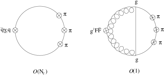
Figure 1: Quark-current and glueball contributions in $\eta\rightarrow\pi\pi\pi$. A similar diagram can be drawn for $\eta^{\prime}$ decays.

The $U(3)$ formalism offers a more complete description of the $\eta$ than the octet theory, because the latter identifies $\eta_{8}$ and $\eta$, neglecting mixing effects that should to be rather important because the mixing angle is not that small. The $U(3)$ calculation improves the tree-level $SU(3)$ prediction for the $\eta\rightarrow\pi\pi\pi$ decays. The most relevant new feature for the these decays seems to be the $\eta-\eta^{\prime}$ mixing (the anomaly does play a role there but it is not a direct contribution to the 4-point function). The mixing angle is well-predicted at leading order and is stable under next-to-leading corrections ($\theta\approx-20^{\circ}/-22^{\circ}$), so significant corrections due to mixing effects are not expected to appear at higher orders. Nevertheless, since the next-to-leading predicted rates stay well below the experimental values, there seems to be no way to avoid the importance of unitary corrections and low-energy resonances whose effects are not included in the effective vertices precisely due to their small mass. The ${\cal O}(\delta^{3})$ effective action would include these final-state-interaction corrections, but tadpole corrections as well as many new terms in the Lagrangian with unknown coupling constants should also be taken into account. If the discrepancies with experimental values are indeed mainly due to the presence of intermediate states, tadpoles and ${\cal O}(\delta^{3})$ counterterms could be safely neglected and the unitary corrections —that can be computed with the known ingredients— should be the only contribution that matters. This one-loop calculation is however out of the scope of the present article and will be left for future work. (A first step in this direction is the evaluation of the one-loop contributions to the masses and decay constants [24]).

The same discussion should also apply to the $\eta^{\prime}\rightarrow\pi\pi\pi$ decays. Although the leading-order approximation produces good estimates of the rates, the emerging pions are far from being soft and this is probably the reason why the expansion apparently blows up when corrections are included.

$\eta^{\prime}\rightarrow\eta\pi\pi$ transitions are probably the most interesting decays in this paper, because this decay could not be analyzed in the framework of $SU(3)$. Momenta are not expected to be too high, so the low-energy expansion might actually work. The results are reasonably good at tree level, but an estimate of the one-loop corrections would also be of great interest in this case, in order to check the convergence of the expansion, which is certainly one the most fragile points in the $U(3)$ theory.

9 Acknowledgments

The author is thankful to J. I. Latorre and J. Taron for suggesting the problem, for their critical reading of the manuscript and for many discussions and comments. She is also grateful to P. Pascual, who took part in some of these discussions and shared his wide experience in the field of particle physics. She also thanks comments and questions from A. Fariborz and D. Black, who also helped with english corrections. The Physics Department of Syracuse University is acknowledged for its hospitality. The project is financially supported by CICYT, contract AEN95-0590, and by CIRIT, contract GRQ93-1047, and by a grant from the Generalitat de Catalunya.

Appendix A Isospin symmetry for $\eta/\eta^{\prime}\rightarrow\pi\pi\pi$ decays

The relation (1) between the charged and the neutral channels can be proved by simply considering isospin symmetry. By definition, for the charged channel,

$$A(s,t,u) = \langle\pi_{0}(p_{1})\ \pi_{+}(p_{2})\ \pi_{-}(p_{3})\ |\ \eta(p_{4})\rangle\;;$$

$$A(t,u,s) = \langle\pi_{0}(p_{2})\ \pi_{+}(p_{3})\ \pi_{-}(p_{1})\ |\ \eta(p_{4})\rangle\;;$$

$$A(u,s,t) = \langle\pi_{0}(p_{3})\ \pi_{+}(p_{1})\ \pi_{-}(p_{2})\ |\ \eta(p_{4})\rangle\;.$$

The permutation of momenta can be viewed as a permutation in the isospin values instead. For instance :

$$|\pi_{0}(p_{2})\ \pi_{+}(p_{3})\ \pi_{-}(p_{1})\ \rangle = -|p_{1}\ p_{2}\ p_{3}\ ;\ 11\ 1{-1}\ 10\ \rangle\;;$$

$$|\pi_{0}(p_{2})\ \pi_{+}(p_{1})\ \pi_{-}(p_{2})\ \rangle = -|p_{1}\ p_{2}\ p_{3}\ ;\ 11\ 10\ 1{-1}\ \rangle\;;$$

$$\vdots$$

These three particle states can be expressed in the Clebsch-Gordan basis $|I^{(2,3)}\ I\ M\rangle$ where the states are labeled in terms of the isospin from particles 2 and 3 $I^{(2,3)}$, the total isospin $I$ and the component in the $z$-direction of the total isospin $I_{z}$.

Due to the bosonic nature of pions, only the totally symmetric states will contribute to the decay amplitude. This restricts the final state to a superposition of three states (expressed in the Clebsch-Gordan basis):

$$|symmetric\,state\rangle=\frac{6}{\sqrt{10}}|2\ 3\ 0\rangle+\frac{4}{\sqrt{15}}|2\ 1\ 0\rangle+\frac{2}{\sqrt{3}}|0\ 1\ 0\rangle\;.$$ (18)

The neutral-channel analysis is much simpler, since all particles are $I=1,\,I_{z}=0$, which can only produce totally symmetric states:

$$|10\ 10\ 10\rangle = \sqrt{\frac{2}{5}}|2\ 3\ 0\rangle-\frac{2}{\sqrt{15}}|2\ 1\ 0\rangle-\frac{2}{\sqrt{3}}|0\ 1\ 0\rangle\;.$$ (19)

However, the $\eta\rightarrow\pi\pi\pi$ transition must be induced by the isospin-violating piece in the QCD Lagrangian [2]:

$${\cal L}_{{\rm QCD}}=-\frac{1}{2}(m_{u}-m_{d})\ (\bar{u}u-\bar{d}d)\;.$$

This is a $\Delta I$=1 operator, so the $I$=3 pieces in (18) and (19) will not contribute to the decay amplitude. The remaining terms differ by the value of $I^{(2,3)}$, so this number can be used to label the two different contributions to the charged amplitude:

$$A(s,t,u) = \langle\ 10\ 11\ 1{-1}\ |\ 00\ \rangle\;=\;\frac{1}{\sqrt{3}}\ A_{0}-\frac{1}{\sqrt{1}5}\ A_{2}\;;$$

$$A(t,u,s) = \langle\ 11\ 1{-1}\ 10\ |\ 00\ \rangle\;=\;\sqrt{\frac{3}{20}}\ A_{2}\;;$$

$$A(s,u,t) = A(s,t,u)\;;$$

$$A(u,t,s) = A(u,s,t)\;=\;A(t,s,u)\;=\;A(t,u,s)\;;$$ (20)

and to the neutral amplitude:

$$\bar{A}(s,t,u) = \langle\ 10\ 10\ 10\ |\ 00\ \rangle\;=\;-\frac{1}{\sqrt{3}}\ A_{0}-\frac{2}{\sqrt{1}5}\ A_{2}\;.$$ (21)

From (20) and (21), it is straightforward to check that:

$$\bar{A}(s,t,u) = A(s,t,u)+A(t,u,s)+A(u,s,t)\;.$$

Obviously the analysis applies to both $\eta$ and $\eta^{\prime}$ decays.

Appendix B Next-to-leading decay amplitudes

The analytical expressions of the decay amplitudes are lengthy due to the dependences on the mixing angle $\theta$. As discussed in the main body of this article, every constant in the computation except $M_{0,0}$ and $L_{3,0}$ can be written in terms of measurable quantities and $\theta$:

$$\Delta_{M} = \frac{3\ M^{2}_{\eta}+M^{2}_{\pi}-4\ M^{2}_{K}+3\ \sin^{2}\theta\ (M^{2}_{\eta^{\prime}}-M^{2}_{\eta})}{4\ (M^{2}_{K}-M^{2}_{\pi})}\;;$$

$$\Delta_{N} = \frac{3}{4\ \sqrt{2}}\ \frac{M^{2}_{\eta^{\prime}}-M^{2}_{\eta}}{M^{2}_{K}-M^{2}_{\pi}}\ \sin 2\theta\;;$$

$$\Delta_{P} = \big{(}\frac{f_{K}}{f_{\pi}}-1\big{)}\;;$$

$$v_{4,0} = -\frac{2}{3}\ \frac{f_{\eta}+f_{\eta^{\prime}}}{f_{\pi}}\ -\ 2\;;$$

The amplitudes will always have the general form:

$$A_{NLO}(\theta) = A_{LO}(\theta)\ +\Delta_{M}(\theta)A_{M}(\theta)+\Delta_{N}(\theta)A_{N}(\theta)+\Delta_{P}A_{P}(\theta)+v_{4,0}A_{4,0}(\theta)$$

$$+ \frac{M_{0,0}}{f^{2}}A_{0,0}(\theta)+\frac{L_{3,0}}{f^{2}}A_{3,0}(\theta)\;,$$

The actual expressions for these next-to-leading contributions to the charged-channel decay amplitudes are given below. The amplitudes for the neutral channels can be inferred from them.

B.1 $\eta\rightarrow\pi\pi\pi$

$$A_{M} = -\frac{2}{3\cos^{2}\theta\ (\sqrt{2}\cos\theta+\sin\theta)^{2}(\cos\theta-\sqrt{2}\sin\theta)}\times$$

$$\Big{(}\ 3s\cos^{2}\theta\ (-2+7\cos^{2}\theta-7\cos^{4}\theta-2\sqrt{2}\sin\theta\cos\theta+4\sin\theta\cos^{3}\theta)$$

$$+ M^{2}_{\pi}\cos\theta\ (35\cos\theta-104\cos^{3}\theta+85\cos^{5}\theta+5\sqrt{2}\sin\theta+12\sqrt{2}\sin\theta\cos^{2}\theta$$

$$- 37\sqrt{2}\sin\theta\cos^{4}\theta)+\frac{M^{4}_{\pi}}{M^{2}_{\eta}-M^{2}_{\pi}}\ (-2-40\cos^{2}\theta+106\cos^{4}\theta-64\cos^{6}\theta$$

$$- 13\sqrt{2}\sin\theta\cos\theta+4\sqrt{2}\sin\theta\cos^{3}\theta+25\sqrt{2}\sin\theta\cos^{5}\theta)\ \Big{)}\;,$$

$$A_{N} = \frac{1}{3(\sqrt{2}\cos\theta+\sin\theta)(\cos\theta-\sqrt{2}\sin\theta)}\times$$

$$\Big{(}-3s\sin 2\theta\ (\cos 2\theta+\frac{\sqrt{2}}{4}\sin 2\theta)+M^{2}_{\pi}\sqrt{2}\ (1+16\cos^{2}\theta-17\cos^{4}\theta)$$

$$+ 10M^{2}_{\pi}\sin\theta\ (3-5\cos^{2}\theta)\ \Big{)}\;,$$

$$A_{P} = -\frac{4}{9\cos^{2}\theta\sin\theta\ (\sin\theta+\sqrt{2}\cos\theta)^{2}(\cos\theta-\sqrt{2}\sin\theta)}\ \frac{M^{2}_{\pi}}{M^{2}_{\eta}-M^{2}_{\pi}}\times$$

$$\Big{(}\ 3s\ (-2\sqrt{2}\cos\theta+5\sqrt{2}\cos^{3}\theta-2\sqrt{2}\cos^{5}\theta-\sqrt{2}\cos^{7}\theta$$

$$- 8\cos^{2}\theta\sin\theta+26\cos^{4}\theta\sin\theta-22\cos^{6}\theta\sin\theta)$$

$$+ M^{2}_{\pi}\ (21\sqrt{2}\cos\theta-37\sqrt{2}\cos^{3}\theta-13\sqrt{2}\cos^{5}\theta+29\sqrt{2}\cos^{7}\theta$$

$$+ 2\sin\theta+72\cos^{2}\theta\sin\theta-210\cos^{4}\theta\sin\theta+152\cos^{6}\theta\sin\theta)\Big{)}\;,$$

$$A_{4,0} = -\frac{3}{2}\ A_{N}\;,$$

$$A_{0,0} = 8\ \sin\theta\ (4\sqrt{2}\cos\theta+\sin\theta)\ \Big{(}s^{2}-3ss_{0}-ut+3M_{2}^{2}\Big{)}\;,$$

$$A_{3,0} = \frac{4}{3\cos\theta(\cos\theta-\sqrt{2}\sin\theta)}\Big{(}\ \cos\theta\ (s^{2}-15ss_{0}+2tu)$$

$$- \cos\theta\sin^{2}\theta\ (42M_{2}^{2}+13s^{2}+57ss_{0}-16tu)-2\sqrt{2}\sin\theta\ (3M_{2}^{2}+s^{2}+3ss_{0}-tu)$$

$$+ 2\sqrt{2}\sin\theta\cos^{2}\theta\ (15M_{2}^{2}+4s^{2}+30ss_{0}-7tu)\Big{)}\;,$$

where $s_{0}=M^{2}_{\eta}/3+M^{2}_{\pi}$ and $M_{2}^{2}=M^{2}_{\pi}\ (M^{2}_{\eta}+M^{2}_{\pi})$.

B.2 $\eta^{\prime}\rightarrow\pi\pi\pi$

$$A_{M} = \frac{2}{9\cos\theta\sin\theta(\cos\theta-\sqrt{2}\sin\theta)^{2}}\times$$

$$\Big{(}9s\ (-3\cos\theta+8\cos^{3}\theta-5\cos^{5}\theta-\sqrt{2}\sin\theta+2\sqrt{2}\cos^{2}\theta\sin\theta-\sqrt{2}\cos^{4}\theta\sin\theta)$$

$$+ \frac{4\ M^{4}_{\pi}}{M^{2}_{\eta^{\prime}}-M^{2}_{\pi}}\ (-16\cos\theta+56\cos^{3}\theta-38\cos^{5}\theta+2\sqrt{2}\cos^{2}\theta\sin\theta-13\sqrt{2}\cos^{4}\theta\sin\theta)$$

$$+ M^{2}_{\pi}(92\cos\theta-267\cos^{3}\theta+175\cos^{5}\theta+28\sqrt{2}\sin\theta-71\sqrt{2}\cos^{2}\theta\sin\theta$$

$$+ 62\sqrt{2}\cos^{4}\theta\sin\theta)\Big{)}\;,$$

$$A_{N} = \frac{1}{3(\cos\theta-\sqrt{2}\sin\theta)}\Big{(}M^{2}_{\pi}\ (\sqrt{2}\cos^{2}\theta-10\sqrt{2}\sin^{2}\theta-28\sin\theta\cos\theta)$$

$$+ 3s\sin\theta\ (\sqrt{2}\sin\theta+2\cos\theta)\Big{)}\;,$$

$$A_{P} = -\frac{4}{9\sin\theta\cos\theta(\cos\theta-\sqrt{2}\sin\theta)^{3}}\ \frac{M^{2}_{\pi}}{M^{2}_{\eta^{\prime}}-M^{2}_{\pi}}\times$$

$$\Big{(}M^{2}_{\pi}\ (-16+108\cos^{2}\theta-246\cos^{4}\theta+152\cos^{6}\theta-24\sqrt{2}\cos\theta\sin\theta$$

$$+ 74\sqrt{2}\cos^{3}\theta\sin\theta-29\sqrt{2}\cos^{5}\theta\sin\theta)-3s(-4+22\cos^{2}\theta-40\cos^{4}\theta+22\cos^{6}\theta$$

$$- 2\sqrt{2}\cos\theta\sin\theta+5\sqrt{2}\cos^{3}\theta\sin\theta-\sqrt{2}\cos^{5}\theta\sin\theta)\Big{)}\;,$$

$$A_{4,0} = -\frac{3}{2}\ A_{N}\;,$$

$$A_{0,0} = \frac{8(\sin\theta+\sqrt{2}\cos\theta)(4\sqrt{2}\sin\theta-\cos\theta)}{\cos\theta-\sqrt{2}\sin\theta}\ \Big{(}s^{2}-3ss_{0}-ut+3M_{2}^{2}\Big{)}\;,$$

$$A_{3,0} = \frac{4}{3\cos\theta(\cos\theta-\sqrt{2}\sin\theta)}\ \Big{(}-\sin\theta\ (s^{2}-15ss_{0}+2tu)$$

$$+ \sin\theta\cos^{2}\theta\ (42M_{2}^{2}+13s^{2}+57ss_{0}-16tu)-2\sqrt{2}\sin\theta\ (3M_{2}^{2}+s^{2}+3ss_{0}-tu)$$

$$+ 2\sqrt{2}\cos\theta\sin^{2}\theta\ (15M_{2}^{2}+4s^{2}+30ss_{0}-7tu)\Big{)}\;,$$

where $s_{0}=M^{2}_{\eta^{\prime}}/3+M^{2}_{\pi}$ and $M_{2}^{2}=M^{2}_{\pi}\ (M^{2}_{\eta^{\prime}}+M^{2}_{\pi})$.

B.3 $\eta^{\prime}\rightarrow\eta\pi\pi$

$$A_{M} = -\frac{8}{9\cos\theta}\ \frac{M^{4}_{\pi}}{M^{2}_{\eta}-M^{2}_{\pi}}\ (2\sqrt{2}\cos^{3}\theta+2\sin^{3}\theta-3\sqrt{2}\cos\theta\sin^{2}\theta)\;,$$

$$A_{N} = \frac{M^{2}_{\pi}}{3}\ (\sqrt{2}\cos 2\theta-2\sin 2\theta)\;,$$

$$A_{P} = \frac{2}{9\cos\theta(\sqrt{2}\cos\theta+\sin\theta)}\ \frac{M^{2}_{\pi}}{M^{2}_{\eta}-M^{2}_{\pi}}\ \Big{(}4M^{2}_{\pi}-2\cos^{2}\theta\ (3M^{2}_{\eta}-6M^{2}_{\eta^{\prime}}+M^{2}_{\pi})$$

$$+ 4\cos^{4}\theta\ (3M^{2}_{\eta}-3M^{2}_{\eta^{\prime}}-4M^{2}_{\pi})+\sqrt{2}\cos\theta\sin\theta\ (3M^{2}_{\eta^{\prime}}+7M^{2}_{\pi})$$

$$+ \sqrt{2}\cos^{3}\theta\sin\theta\ (-3M^{2}_{\eta}+3M^{2}_{\eta^{\prime}}-14M^{2}_{\pi})\Big{)}\;,$$

$$A_{4,0} = -\frac{3}{2}\ A_{N}\;,$$

$$A_{0,0} = -4\ (2\sqrt{2}\cos 2\theta-\sin 2\theta)\ \Big{(}M^{4}_{\pi}+2M^{2}_{\pi}(M^{2}_{\eta}+M^{2}_{\eta^{\prime}})+M^{2}_{\eta}M^{2}_{\eta^{\prime}}+s^{2}-tu+3ss_{0}\Big{)}\;,$$

$$A_{3,0} = \frac{1}{3}\ A_{0,0}\;,$$

where $s_{0}=(M^{2}_{\eta^{\prime}}+M^{2}_{\eta}+2M^{2}_{\pi})/3$.

References

- [1] Eur.Phys.J. C3 (1998)
- [2] J. Gasser and H. Leutwyler, Nucl. Phys. B250 (1985) 539.
-
[3]
J. J. Sakurai, Ann. Phys. 11 (1960) 1;
Y. Nambu, J. J. Sakurai, Phys. Rev. Lett. 8 (1962) 79, 191 E;
M. Gell-Mann, D. Sharp, W. Wagner, Phys. Rev. Lett. 8 (1962) 261;
J. J. Sakurai, Currents and Mesons, University of Chicago Press (1969). - [4] M. Harada, F. Sannino, J. Schechter, Phys. Rev. D54 (1996) 1991.
- [5] J. A. Oller, E. Oset, Nucl. Phys. A620 (1997) 438.
- [6] A. Pich, -Decays and Chiral Lagrangians, talk given at the Workshop on Rare Decays of Light Mesons, Gif-sur-Yvette, France, Mar 29-30, 1990, published in Gif Workshop 1990:0043-52.
- [7] P. Herrera-Siklódy, J. I. Latorre, P. Pascual and J. Taron, Nucl. Phys. B497 (1997) 345.
- [8] P. Herrera-Siklódy, J. I. Latorre, P. Pascual and J. Taron, Phys. Lett. B419 (1998) 326.
- [9] H. Leutwyler, Phys. Lett. B374 (1996) 163.
- [10] P. Herrera-Siklódy, Phys.Lett.B 442 (1998) 359.
- [11] A. Pich, Effective Field Theory, course given in Les Houches Summer School 1997, hep-ph/9806303, to be published by Elsevier Science B.V.
-
[12]
J. Balog, Phys. Lett.
B149 (1984) 197;
A. A. Andrianov, Phys. Lett. B157 (1985) 425;
D.Espriu, E. de Rafael, J.Taron, Nucl. Phys. B 345 (1990) 22;
J.Bijnens, C. Bruno, E. de Rafael, Nucl. Phys. B 390 (1993) 501. - [13] S. Weinberg Phys. Rev. D11 (1975) 3583.
- [14] J. Gasser and H. Leutwyler, Nucl. Phys. B250 (1985) 465.
- [15] C. Roisnel, T. N. Truong, Nucl. Phys. B187 (1981) 293.
- [16] S. Fajfer, J.-M. Gérard, Z. Phys. C42 (1989) 431.
- [17] R. Akhoury, J-. M. Frère, Phys. Lett. B 220 (1989) 258.
-
[18]
Riazuddin, S. Oneida, Phys. Rev. Lett. 27
(1971) 549;
P. Weisz, Riazuddin, S. Oneida Phys. Rev. D5 (1972) 2264. - [19] P. Di Vecchia, F. Nicodemi, R. Pettorino and G. Veneziano, Nucl. Phys. B181 (1981) 318.
- [20] R. Akhoury, M. Leurer, Z. Phys. C43 (1989) 145.
- [21] A. H. Fariborz, J. Schechter, hep-ph/9902238.
-
[22]
N. G. Deshpande, T. N. Truong, Phys. Rev. Lett. 41
(1978) 1579;
P. Castoldi, J. -M. Frère, Z. Phys. C40 (1988)283;
C. A. Singh, J. Pasupathy, Phys. Rev. Lett. 35 (1975) 1193. - [23] G. Ecker et al., Nucl. Phys. B321 (1989) 311.
- [24] R. Kaiser, H. Leutwyler, hep-ph/9806336.