Magnetic Fields from Bubble Collisions —
A Progress Report

Ola Törnkvist
Department of Applied Mathematics and Theoretical Physics,
University of Cambridge,
Silver Street, Cambridge CB3 9EW, United Kingdom
15 February 1999

Abstract

Primordial magnetic fields may be created in collisions of expanding bubbles in a first-order cosmological phase transition and later serve as seed fields for galactic magnetic fields. Here I present results from numerical and analytical studies of U(1) bubble collisions done in collaboration with Ed Copeland and Paul Saffin. I also reveal preliminary results from analytical studies of SU(2)$\times$U(1) bubble collisions, which provide first evidence that magnetic fields are created in electroweak two-bubble collisions.

1 Introduction

Observations show that magnetic field strengths of the order of $10^{-6}$ Gauss are typical in spiral galaxies. Because the fields appear aligned with the rotational plane of each galaxy, a plausible explanation is that they were created by a dynamo mechanism, in which a weak seed field was exponentially amplified by the turbulent motion of ionised gas in conjunction with the differential rotation of the galaxy. There have been many proposals for seed fields [1]; here I shall concentrate on the generation of magnetic fields in bubble collisions in the electroweak phase transition (EWPT). Although there is no consensus that such seed fields would be sufficiently strong and correlated [2], recent results indicate that the present theoretical bounds on seed fields are too stringent [3].

Because there is no EWPT in the Standard Model (SM) [4], we need to consider a two-Higgs model such as the Minimal Supersymmetric Standard Model (MSSM), which permits a strong first-order transition for Higgs-boson mass $M_{h}\lower 3.01385pt\hbox{$\;\stackrel{{\scriptstyle\textstyle<}}{{\sim}}\;$}105-116$ GeV [5]. For the purpose of bubble nucleation a more weakly first-order transition will suffice, and consequently higher values of $M_{h}$ are allowed. A general (non-supersymmetric) two-Higgs model can easily accommodate a first-order transition within its extensive parameter space.

Because two-Higgs models and the SM have the same Higgs vacuum manifold $S^{3}$, bubble collisions in these models are expected to be very similar, and we can focus our attention on the more tractable SM problem. In these investigations we ignore plasma friction and the dissipation due to Ohmic currents.

2 Bubble Collisions in a U(1) Model

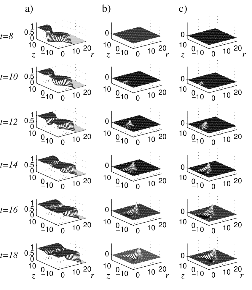
Figure 1: Bubble collision in a U(1) model: Evolution of a) modulus of the Higgs field, b) the azimuthal field strength $F_{rz}$ in a numerical simulation. c) Analytical solution. Here $r=(x^{2}+y^{2})^{1/2}$ is the distance from the axis of the collision, and $r$, $z$, $t$ are measured in units of $2M_{h}^{-1}$. The centres of the two bubbles are at $r=0$, $z=\pm 12.5$. The collision occurs shortly before $t=10$. A colour version of this figure can be viewed and downloaded at http://www.damtp.cam.ac.uk/user/ot202/sewm98/

Let us first consider a U(1) model and the collision of two bubbles with Higgs fields $\phi_{1}=\rho_{1}(x)e^{i\theta_{1}}$ and $\phi_{2}=\rho_{2}(x)e^{i\theta_{2}}$, respectively, and constant phases $\theta_{1}\neq\theta_{2}$. In order to model the generation of magnetic fields, we set the initial U(1) field strength to zero. One may then choose a gauge in which the vector potential $V_{\mu}$ is initially zero. Because of the phase gradient, a gauge-invariant current $j_{k}=iq[\phi^{\dagger}D_{k}\phi-(D_{k}\phi)^{\dagger}\phi]$ develops across the surface of intersection of the two bubbles, where $D_{k}=\partial_{k}-iqV_{k}$. The current gives rise to a ring-like flux of the field strength $F_{ij}=\partial_{i}V_{j}-\partial_{j}V_{i}$ which takes the shape of a girdle encircling the bubble intersection region. The time evolution of the azimuthal field strength, as obtained in recent numerical simulations [6], is shown in Fig. 1b. An approximate time-dependent solution was first obtained by Kibble and Vilenkin [7], who set the modulus of the Higgs field equal to its vacuum expectation value. Because they used a step function as initial condition for the phase of the Higgs field, their solution suffers from discontinuities on the future null surface of bubble intersections.

We have obtained a different analytical solution by taking into account the profile of the Higgs modulus for each bubble and deriving smooth initial conditions from a superposition ansatz [6]. These analytical results can be seen in Fig. 1c and may be compared with the exact evolution in Fig. 1b. The magnetic field is concentrated in a narrow flux tube along the circle of most recent intersection of the two bubbles. From the analytical solutions we find that the tube’s radial width is $\Delta r\sim m^{-1}t_{\rm coll}/t$ and the maximal field strength is $B_{\rm max}\sim|\theta_{2}-\theta_{1}|m^{2}r(t)/(2qt_{\rm coll})$, where $t_{\rm coll}$ is the time of collision, $r(t)$ is the bubble radius, and $m$ is the vector-boson mass. The total flux tends to a constant $(\theta_{2}-\theta_{1})/q$ at large times [7]. The narrowing of the flux tube and increase of field strength with time is a result of Lorentz contraction as the bubble walls accelerate in the absence of friction.

3 Magnetic Fields from SU(2)$\times$U(1) Bubble Collisions

In electroweak bubble collisions the initial Higgs field in the two bubbles is of the form

$$\Phi_{1}=\Big{(}\!\begin{array}[]{c}0\\[-2.84526pt] \rho_{1}(x)\end{array}\!\Big{)}~{},\quad\quad\Phi_{2}=\exp(i\textstyle{\theta_{0}}{\mbox{\boldmath$n$}}\cdot{\mbox{\boldmath$\tau$}})\Big{(}\!\begin{array}[]{c}0\\[-2.84526pt] \rho_{2}(x)\end{array}\!\Big{)}~{},$$ (1)

respectively. A constant SU(2) matrix $\exp(i\textstyle{\theta_{0}}{\mbox{\boldmath$n$}}\cdot{\mbox{\boldmath$\tau$}})$ has here replaced the phase $e^{i\theta_{0}}$ of the U(1) model. Saffin and Copeland have found that the initial Higgs-field configuration can be written globally as [8]

$$\Phi(x)=\exp(i\textstyle{\theta(x)}{\mbox{\boldmath$n$}}\cdot{\mbox{\boldmath$\tau$}})\Big{(}\!\begin{array}[]{c}0\\[-2.84526pt] \rho(x)\end{array}\!\Big{)}~{},$$ (2)

where $n$ is the same constant unit vector as in Eq. (1). As the bubbles collide, non-Abelian currents $j^{A}_{k}=i[\Phi^{\dagger}T^{A}D_{k}\Phi-(D_{k}\Phi)^{\dagger}T^{A}\Phi]$ develop across the surface of intersection of the two bubbles, where $T^{A}=(g^{\prime}/2,g\tau^{a}/2)$, $D_{k}=\partial_{k}-iW_{k}^{A}T^{A}$ and $W^{A}_{k}=(Y_{k},W^{a}_{k})$. In analogy with the U(1) case, one obtains here a ringlike flux, but this time of non-Abelian field strengths. The important question is then how to project out the electromagnetic field in a gauge-invariant way. In recent work [9] I have shown how to construct from first principles an electromagnetic U(1) vector potential, unique up to a gradient, whose curl in any gauge of SU(2)$\times$U(1) gives the electromagnetic (EM) field tensor. In terms of the 3-component unit isovector $\hat{\phi}^{a}=(\Phi^{\dagger}\tau^{a}\Phi)/(\Phi^{\dagger}\Phi)$ this vector potential is given by

$$A^{\rm em}_{\mu}=-\sin\theta_{\!\rm w\,}\hat{\phi}^{a}W^{a}_{\mu}+\cos\theta_{\!\rm w\,}Y_{\mu}-\frac{\sin\theta_{\!\rm w\,}}{g}\frac{\epsilon^{abc}s^{a}\hat{\phi}^{b}\partial_{\mu}\hat{\phi}^{c}}{1-s^{d}\hat{\phi}^{d}}~{},$$ (3)

where ${\mbox{\boldmath$s$}}=\{s^{a}\}$ is an arbitrary constant unit vector. It is not hard to show that $A^{\rm em}_{\mu}$ transforms only by a pure gradient under general SU(2)$\times$U(1) gauge transformations (or a change of $s$). The line integral of $A^{\rm em}_{\mu}$ along a closed curve therefore gives the gauge-invariant EM flux. The gauge-invariant EM field tensor ${\cal F}^{\rm em}_{\mu\nu}\equiv\partial_{\mu}A^{\rm em}_{\nu}-\partial_{\nu}A^{\rm em}_{\mu}$ becomes [9]

$${\cal F}^{\rm em}_{\mu\nu}=-\sin\theta_{\!\rm w\,}\partial_{[\mu}(\hat{\phi}^{a}W^{a}_{\nu]})+\cos\theta_{\!\rm w\,}F^{Y}_{\mu\nu}+\textstyle\frac{\sin\theta_{\!\rm w\,}}{g}\epsilon^{abc}\hat{\phi}^{a}(\partial_{\mu}\hat{\phi})^{b}(\partial_{\nu}\hat{\phi})^{c}~{}.$$ (4)

It is important to note that ${\cal F}^{\rm em}_{\mu\nu}$ receives contributions from Higgs-field gradients. The benefits of definition (4) as compared with other proposed definitions have been discussed thoroughly in Refs. 9 and 10.

We now return to the issue of bubble collisions. As in the U(1) case one may assume that the initial configuration has zero field strengths and zero vector potentials, $F^{a}_{\mu\nu}=F^{Y}_{\mu\nu}=W_{\mu}^{a}=Y_{\mu}=0$. The only possible contribution to the EM field tensor then comes from the last term in Eq. (4). However, for $\hat{\phi}^{a}$ corresponding to the initial Higgs configuration Eq. (2), this term is zero [10]. The simple reason is that $\hat{\phi}^{a}$ depends on the spacetime coordinates $x$ only through one scalar function $\theta(x)$, and no antisymmetric tensor can be constructed from its derivatives. Similarly I have shown that, as long as the field configuration maintains the simple form (2), the electric current vanishes [10]. From Maxwell’s equations one then finds that the time derivatives of both electric and magnetic fields are zero.

It would then seem as though no magnetic fields are generated in electroweak two-bubble collisions. This is indeed what I find using the linearised equations to calculate analytically the field evolution beyond initial times. However, there is a magnetic field proportional to $n_{3}(1-n_{3}^{\,\,2})\sin^{3}\theta_{\!\rm w\,}/g$ generated to first order in the nonlinearities by a current produced by the initially excited W and Z fields. The current arises because of the difference in the evolution of the W and Z mass eigenstates. This first-order correction is furthermore characterised by a rotational motion in the $(W^{1},W^{2})$ isoplane. The resulting current generates a magnetic field to second order in the nonlinearities.

By contrast, in a collision of three bubbles a magnetic field is present already in the initial field configuration. Labelling the bubbles by 0, 1, and 2, we denote the Higgs field in each bubble by $\Phi_{i}=U_{i}(0,\rho_{i}(x))^{\top}$, where $U_{0}=1$, $U_{1}=\exp(i\theta_{1}{\mbox{\boldmath$m$}}\cdot{\mbox{\boldmath$\tau$}})$, and $U_{2}=\exp(i\theta_{2}{\mbox{\boldmath$n$}}\cdot{\mbox{\boldmath$\tau$}})$ are constant SU(2) matrices with linearly independent unit vectors $m$, $n$. The initial Higgs field can here be written globally as $\Phi=\exp[i(f(x)m_{a}+g(x)n_{a})\tau^{a}](0,\rho(x))^{\top}$, where $f,g=\sin\theta_{1,2}\rho_{1,2}\Theta/(\rho\sin\Theta)$, $\cos\Theta=\sum_{i}\rho_{i}\cos\theta_{i}/\rho$ and $\rho^{2}=\sum_{i}\rho_{i}^{2}+2\sum_{i<j}\rho_{i}\rho_{j}(\cos\theta_{i}\cos\theta_{j}+{\mbox{\boldmath$m$}}\cdot{\mbox{\boldmath$n$}}\sin\theta_{i}\sin\theta_{j})$ with $\theta_{0}=0$. From Eq. (4) the initial electromagnetic field then becomes

$${\cal F}^{\rm em}_{\mu\nu}=\textstyle-\frac{4\sin\theta_{\!\rm w\,}}{g}f_{[,\mu}g_{,\nu]}\,\,\hat{{\mbox{\boldmath$e$}}}_{3}\cdot\!\left(\frac{\sin 2\Theta}{2\Theta}({\mbox{\boldmath$m$}}\!\times\!{\mbox{\boldmath$n$}})+\frac{\sin^{2}\Theta}{\Theta^{2}}(f{\mbox{\boldmath$m$}}\!+\!g{\mbox{\boldmath$n$}})\!\times\!({\mbox{\boldmath$m$}}\!\times\!{\mbox{\boldmath$n$}})\right)~{},$$ (5)

which comprises a nonzero magnetic field as long as $\nabla f\times\nabla g\neq 0$. The three-bubble mechanism is, however, suppressed, as the third bubble must impinge before the SU(2) phases of the first two have equilibrated, and such nearly simultaneous collisions are rare.

If $m$ and $n$ are collinear, ${\cal F}^{\rm em}_{\mu\nu}$ vanishes. More generally, one can show that the EM field and the current are zero only when the SU(2) phases of the Higgs field take values along one single geodesic on the Higgs vacuum manifold, such as is generated by the exponentiation of one Lie-algebra element (cf. Eq. (2)).

References

- [1] Due to lack of space here, please see references given in [10] below.
- [2] D.T. Son, hep-ph/9803412.
- [3] M.J. Lilley, O. Törnkvist, and A.-C. Davis, in preparation.
- [4] K. Kajantie, M. Laine, K. Rummukainen and M. Shaposhnikov, Phys. Rev. Lett. 77, 2887 (1996); F. Csikor, Z. Fodor and J. Heitger, Phys. Rev. Lett. 82, 21 (1999).
- [5] M. Laine and K. Rummukainen, Phys. Rev. Lett. 80 5259 (1998); J.M. Cline and G.D. Moore, Phys. Rev. Lett. 81, 3315 (1998).
- [6] E.J. Copeland, P.M. Saffin, and O. Törnkvist, in preparation.
- [7] T.W.B. Kibble, A. Vilenkin, Phys. Rev. D52, 679 (1995).
- [8] P.M. Saffin and E.J. Copeland, Phys. Rev. D56, 1215 (1997).
- [9] O. Törnkvist, hep-ph/9805255.
- [10] O. Törnkvist, Phys. Rev. D58, 043501 (1998).