Renormalization Group Effects in the Process $H\longrightarrow\gamma\gamma$
Michael Melles
Department of Physics, University of Durham, Durham DH1 3LE, U.K.

Abstract

The partial Higgs width $\Gamma(H\longrightarrow\gamma\gamma)$ is important at the LHC for Higgs masses in the MSSM mass window up to $140$ GeV as a relatively background free signal of a fundamental scalar. At the photon photon mode at the NLC it would be the Higgs production mechanism. Two loop QCD corrections exist for the fermionic contribution and in the case of the bottom loop large non-Sudakov double logarithms can be resummed to all orders and contribute up to 12 % compared to the t-quark. In more complicated Higgs sectors, such as in the MSSM, large $\tan\beta$ enhancements of bottom type Yukawa couplings can potentially dominate even the whole partial width. A main uncertainty in all existing calculations is the scale of the strong coupling as it is only renormalized at the three loop level. In this paper we include the exact two loop running coupling to all orders into the bottom contribution. We find that the effective scale is close to $\alpha_{s}(10m_{b}^{2})$.

1 Introduction

The investigation of the electroweak symmetry breaking sector is certain to dominate both theoretical as well as experimental high energy physics through the coming decade. High precision measurements of electroweak observables at the SLC and LEP indicate that the Standard Model Higgs boson has a mass between $95$-$280$ GeV at the $95$% confidence level with a preference towards the lower mass regime [1]. While the Standard Model (SM) has enjoyed spectacular theoretical success, the Higgs sector of the theory is the only aspect for which no “standard” in the experimentally tested sense has yet been set. The simplest ansatz for the Higgs sector, assumed in the SM, leads to only one neutral fundamental scalar but several more complicated scenarios are a priori just as viable. Well known examples include a general two doublet Higgs model [2, 3, 4] and the Higgs sector of the minimal supersymmetric extension of the SM (MSSM) [5].

A common feature of all phenomenologically viable extensions of the SM Higgs sector must be the existence of a “SM-like” neutral scalar in the SLC/LEP mass window. In the case of the MSSM, the lightest neutral scalar must be lighter than the Z-boson mass [6]. Radiative corrections allow its mass to reach at most $130$-$140$ GeV. The introduction of additional singlet Higgs bosons can of course soften this upper bound somewhat, depending mainly on the value of the stop mass [7], but at least the MSSM would be ruled out for higher masses of the lightest neutral scalar.

Among the experimentally observable Higgs signals the $H\longrightarrow\gamma\gamma$ coupling is of considerable interest. At the LHC it can be used as a relatively background free process [8]. For Higgs masses in the MSSM regime it is actually the only feasible signal due to the large QCD background of other processes. Excellent energy and angular resolutions of the detectors allow to discriminate the photon photon decay against the continuum QCD background [9, 10]. At the photon photon mode of the NLC it would be the primary resonance production process [11, 12, 13].

While the charged gauge boson loop gives the largest contribution in the SM [5, 8], the fermion loops deserve special attention. Radiation of a single gluon is not possible due to charge conjugation invariance and color conservation. For the partial width $\Gamma(H\longrightarrow\gamma\gamma)$ the fermion loops interfere destructively and for large Higgs masses ($\sim$600 GeV) the top loop nearly cancels the $W$ loop contribution. In that case the bottom loop would be artificially “enhanced” in terms of its phenomenological importance. There is of course also the possibility of $t$ and $b$ “colluding” in their destructive interference with the charged gauge boson loop.

In the SM, the top quark loop yields the bulk (almost 90%) of the fermionic contribution to $\Gamma(H\longrightarrow\gamma\gamma)$ due to the large Yukawa coupling. The bottom quark contribution is still significant ( 12%) due to larger radiative corrections expounded on below [14]. In order to constrain new physics the theoretical SM-predictions should be as precise as possible. One main source of uncertainty in the bottom quark contribution is the fact that the strong coupling $\alpha_{s}$ receives no renormalization through two loops. The same is of course also true for the top quark loop, however, the change in $\alpha_{s}$ between the two mass scales is much smaller and the radiative corrections are also not as large in relative terms [14]. The width contribution stemming from a bottom quark, however, changes up to $17\%$ for a Higgs boson mass below the $W^{\pm}$ threshold depending on whether one chooses to evaluate $\alpha_{s}$ at $m_{b}^{2}$ or $m_{H}^{2}$.

Tackling this uncertainty is the purpose of this work. There are two other circumstances in which a renormalization group improvement is crucial. Firstly for the case of the second heavy neutral scalar predicted in any model with two complex doublets. In this scenario the aforementioned large radiative corrections would be even bigger and the clear signal identification at a future collider would hence benefit from a precise knowledge of QCD corrections. The second and possibly much more important circumstance is that of a large $\tan\beta$ enhancement of bottom type Yukawa couplings. These typically enter for two doublet Higgs sectors with a $\frac{1}{\cos\beta}$ factor in the coupling [5]. Phenomenological restrictions lead to a range roughly between $1<\tan\beta<50$ [15]. As the width is proportional to the square of $\frac{1}{\cos\beta}$, any enhancement of the coupling could be substantial, even dominating. Lastly it is also theoretically of interest to study the effect of renormalization group improvements for processes involving Yukawa couplings.

In the next section we briefly review the radiative corrections for the case of the bottom contribution. Although an exact two loop calculation exists [16], the largest contribution is contained in non-Sudakov double logarithms (DL’s) and we will only review this calculation as it allows for an all orders inclusion of the renormalization group effects. The derivation of the running coupling improved form factor is then given based on a topological similarity between the $H\gamma\gamma$ and the Sudakov vertex in terms of their double logarithmic content up to the last loop integration. We then compare the renormalization group improved form factor with effective couplings in the DL approximation and make concluding remarks about the generality of the presented results.

2 Renormalization Group Improved Form Factor

In this section we drop the index $m_{b}$ as it is unnecessary in that all results derived are valid whenever the ratio $\frac{m^{2}}{m_{H}^{2}}$ leads to large logarithms. For phenomenological applications we have the b-quark in mind. We also explicitly only discuss the SM case. The only change for more complicated Higgs sectors for the neutral scalars would be in the Yukawa coupling. All DL-form factors and renormalization group effects would remain unchanged.

It was shown in Ref. [17] that in the case of a small ratio of $\frac{m^{2}}{m_{H}^{2}}$ large non-Sudakov double logarithms occur in the amplitude $H\longrightarrow\gamma\gamma$ via a fermion loop. The resulting series can be expressed in the following form:

$${\cal M}_{q}^{DL}(H\longrightarrow\gamma\gamma)=e^{*}_{1\mu}e^{*}_{2\nu}\left(\frac{m^{2}_{H}}{2}g^{\mu\nu}-k^{\mu}_{2}k^{\nu}_{1}\right)\sqrt{\sqrt{2}G_{F}}\frac{e^{2}}{(4\pi)^{2}}N_{c}\sum_{q}Q^{2}_{q}{\cal F}_{H}^{DL}$$ (1)

where $e_{1,2}$, $k_{1,2}$ are the polarization vectors and four-momenta of the photons, $N_{c}$ the number of colors and $Q_{q}$ the electric charge of quark $q$ in units of the charge of the positron $e$. The double logarithmic form factor is given by

$${\cal F}_{H}^{DL}=\frac{4m^{2}}{m_{H}^{2}}\log^{2}\frac{m^{2}}{m^{2}_{H}}\sum^{\infty}_{n=0}\frac{2\Gamma(n+1)}{\Gamma(2n+3)}\left(-\frac{\alpha_{s}C_{F}}{2\pi}\log^{2}\frac{m^{2}}{m^{2}_{H}}\right)^{n}$$ (2)

The leading order partial Higgs width was first given in Ref. [18]. In order to improve the perturbative behavior of the quark loop contribution one should use running quark masses with $m\left(\frac{m_{H}}{2}\right)$ as the effective scale for the photonic decay mode [8]. Within the DL approximation the scale at which to evaluate the QCD-coupling $\alpha_{s}$, however, is unrestricted. Even for an exact calculation of the two $\gamma$ partial Higgs width the strong coupling is only renormalized at the three loop level. As mentioned above, this inherent ambiguity leads to up to $17\%$ uncertainty in the bottom contribution to the partial width $\Gamma(H\longrightarrow\gamma\gamma)$ for an intermediate mass Higgs boson. In the following we will derive the renormalization group effects of inserting a running coupling into each loop evaluation for the exact one- and two-loop solution of the $\beta$-function. All higher order RG-terms would then be suppressed by $\frac{1}{\log^{3}\frac{s}{m^{2}}}$.

In the derivation of the leading logarithmic corrections in Ref. [17] the familiar Sudakov technique [19, 20, 21] was used by decomposing loop momenta into components along external momenta , denoted by $\{\alpha,\beta\}$ and those perpendicular to them, denoted by $l_{\perp}$. Integrating first over the perpendicular components as usual, the double logarithmic form factor of Eq. 2 was derived from a double integral over the Sudakov form factor:

$${\cal F}_{H}^{DL}=\frac{4m^{2}}{m^{2}_{H}}\int^{1}_{-1}\int^{1}_{-1}\frac{d\alpha}{\alpha}\frac{d\beta}{\beta}\Theta\left(\alpha\beta-\frac{m^{2}}{m^{2}_{H}}\right)\exp\left[-\frac{\alpha_{s}C_{F}}{2\pi}\log|\alpha|\log|\beta|\right]$$ (3)

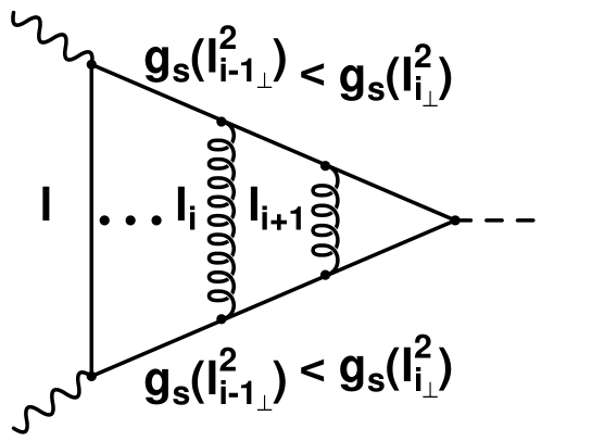
Figure 1: The schematic Feynman diagrams leading to the hard (non-Sudakov) double logarithms in the partial width $\Gamma(H\longrightarrow\gamma\gamma)$ with $i+1$ gluon insertions. Crossed diagrams lead to a different ordering of the Sudakov variables and are correctly accounted for by a factor of $(i+1)!$ at each order. The scale of the coupling $\alpha_{s}=\frac{g_{s}^{2}}{4\pi}$ is indicated at the vertices and included in this work.

We want to emphasize at this point that ideally one would like to have an explicit three loop calculation in order to determine the effective scale at the two loop level for a renormalization group improvement to all orders. Without such a calculation is seems hard to attempt a rigorous inclusion of the running coupling, however, the form of the derivation of the non-Sudakov DL’s in Eq. 3 is the key point. For Sudakov double logarithms the relevant scale for the coupling at each loop is $\alpha_{s}(l^{2}_{\perp})$ as was shown in Refs. [22, 23, 24]. Following similar arguments we find that the same is true for the novel non-Sudakov logarithms given in Eq. 2. One way to see this is the fact that on a formal level, all insertions of gluons into the DL-topology shown in Fig. 1 have the same structure as in the Sudakov case. Eq. 3 is the explicit mathematical formulation of this fact. Only the last fermion loop integration separates the two cases by effectively regularizing soft divergences with the quark mass. The strong coupling receives no renormalization from this last integration, however, so that the scales of the couplings at each order are determined by the same renormalization group arguments as for the Sudakov case.

We start by writing

$$\alpha_{s}(l^{2}_{\perp})=\frac{\alpha_{s}(m^{2})}{1+\beta_{0}\frac{\alpha_{s}(m^{2})}{\pi}\log\frac{l^{2}_{\perp}}{m^{2}}+\beta_{1}\left(\frac{\alpha_{s}(m^{2})}{\pi}\right)^{2}\log\frac{l^{2}_{\perp}}{m^{2}}}$$ (4)

where $\beta_{0}=\frac{11}{12}C_{A}-\frac{4}{12}T_{F}n_{F}$, $\beta_{1}=\frac{17}{24}C_{A}^{2}-\frac{5}{12}C_{A}T_{F}n_{F}-\frac{1}{4}C_{F}T_{F}n_{F}$ and for QCD we have $C_{A}=3$, $C_{F}=\frac{4}{3}$ and $T_{F}=\frac{1}{2}$ as usual. Up to two loops the massless $\beta$-function is independent of the chosen renormalization scheme and is gauge invariant in minimally subtracted schemes to all orders [25]. These features will also hold for the derived renormalization group improved form factor below. From the exact next to leading order result in Eq. 4 it is clear that a formulation in terms of $l^{2}_{\perp}$ of the series leading to the non-Sudakov double logarithms is more adaptable to a renormalization group improvement. Eq. 3 can be reformulated in the following form:

$${\cal F}_{H}^{DL}\!\!\! = \!\!\!\!\frac{8m^{2}}{m^{2}_{H}}\sum^{\infty}_{n=1}\int^{m^{2}_{H}}_{m^{2}}\frac{dl^{2}_{\perp}}{l^{2}_{\perp}}\int^{1}_{\frac{l^{2}_{\perp}}{m^{2}_{H}}}\frac{d\alpha}{\alpha}\prod^{n-1}_{i=1}\Gamma(n)\int^{l^{2}_{{i-1}_{\perp}}}_{m^{2}}\frac{dl^{2}_{{i}_{\perp}}}{l^{2}_{{i}_{\perp}}}\int^{1}_{\alpha_{i-1}}\frac{d\alpha_{i}}{\alpha_{i}}\left(\frac{-\alpha_{s}C_{F}}{2\pi}\right)^{n-1}$$ (5)

The product above is set to one for $n=1$ and contains nested integrals for $n\geq 2$ with $l^{2}_{{0}_{\perp}}\equiv l^{2}_{\perp}$ and $\alpha_{0}\equiv\alpha$. From this expression it is clear that an incorporation of the running coupling in Eq. 4 will not contain any Landau pole singularity [26] as $m^{2}\leq l^{2}_{i_{\perp}}\leq l^{2}_{\perp}$. The fact that the strong coupling enters only at two loops means that for $i+1$ gluon insertions the first loop integral leads to a simple logarithm:

$$\int^{l^{2}_{i_{\perp}}}_{m^{2}}\frac{dl^{2}_{{i+1}_{\perp}}}{l^{2}_{{i+1}_{\perp}}}=\log\frac{l^{2}_{i_{\perp}}}{m^{2}}$$ (6)

This is a consequence of the requirement that the effective scale be $l^{2}_{i_{\perp}}$ at the $i+1$-th gluon coupling. Fig. 1 indicates this schematically. For the following integrals we use $c\equiv\left(\beta_{0}\frac{\alpha_{s}(m^{2})}{\pi}+\beta_{1}\left(\frac{\alpha_{s}(m^{2})}{\pi}\right)^{2}\right)$. At the $i$-th order we then have:

$$\int^{l^{2}_{{i-1}_{\perp}}}_{m^{2}}\frac{dl^{2}_{{i}_{\perp}}}{l^{2}_{{i}_{\perp}}}\frac{\alpha_{s}(m^{2})\log\frac{l^{2}_{{i}_{\perp}}}{m^{2}}}{1+c\;\log\frac{l^{2}_{{i}_{\perp}}}{m^{2}}}=-\frac{\alpha_{s}(m^{2})}{c^{2}}\left(\log\frac{\alpha_{s}(m^{2})}{\alpha_{s}(l^{2}_{{i-1}_{\perp}})}-c\log\frac{l^{2}_{{i-1}_{\perp}}}{m^{2}}\right)$$ (7)

While the last term gives the same type of integral in the next step we use for the first contribution on the r.h.s.:

$$\frac{dl^{2}_{i_{\perp}}}{l^{2}_{i_{\perp}}}=-\frac{\alpha_{s}(m^{2})}{c}\frac{d\log(\alpha_{s}(l^{2}_{i_{\perp}}))}{\alpha_{s}(l^{2}_{i_{\perp}})}$$ (8)

and find

$$-\int^{l^{2}_{{i-2}_{\perp}}}_{m^{2}}\frac{dl^{2}_{{i-1}_{\perp}}}{l^{2}_{{i-1}_{\perp}}}\alpha_{s}(l^{2}_{{i-1}_{\perp}})\frac{\alpha_{s}(m^{2})}{c^{2}}\left(\log\frac{\alpha(m^{2})}{\alpha(l^{2}_{{i-1}_{\perp}})}\right)$$ (9)

$$= -\frac{\alpha^{2}_{s}(m^{2})}{2c^{3}}\log^{2}\frac{\alpha(m^{2})}{\alpha(l^{2}_{{i-2}_{\perp}})}$$

It is clear from this derivation at the n-loop level we have

$$\frac{1}{(n-1)!}\left(\frac{\alpha_{s}(m^{2})C_{F}}{2\pi\;c}\right)^{n-1}\left(-\sum^{n-2}_{i=1}\frac{1}{i!}\log^{i}\frac{\alpha_{s}(m^{2})}{\alpha_{s}(l^{2}_{\perp})}+c\;\log\frac{l^{2}_{\perp}}{m^{2}}\right)\frac{\log^{n-1}\alpha}{\alpha}$$ (10)

Thus we finally arrive at the complete renormalization group improved result for the hard non-Sudakov form factor of Fig. 1:

$${\widetilde{\cal F}_{H}^{DL}} = \frac{4m^{2}}{m^{2}_{H}}\left[\log^{2}\frac{s}{m^{2}}-2\sum^{\infty}_{n=2}\int^{s}_{m^{2}}\frac{dl^{2}_{\perp}}{l^{2}_{\perp}}\left(\frac{\alpha_{s}(m^{2})C_{F}}{2\pi\;c}\right)^{n-1}\frac{1}{n}\right.$$ (11)

$$\times\left.\left(-\sum^{n-2}_{i=1}\frac{1}{i!}\log^{i}\frac{\alpha_{s}(m^{2})}{\alpha_{s}(l^{2}_{\perp})}+c\;\log\frac{l^{2}_{\perp}}{m^{2}}\right)\frac{\log^{n}\frac{l^{2}_{\perp}}{s}}{1+c\;\log\frac{l^{2}_{\perp}}{m^{2}}}\right]$$

An expansion in $\alpha_{s}(m^{2})$ gives the double logarithmic form factor in Eq. 2 plus subleading terms proportional to $\beta_{0}$ etc.. The bottom contribution to the width is thus proportional to

$$\Gamma^{DL}_{b}(H\longrightarrow\gamma\gamma)\sim|{\widetilde{\cal F}_{H}^{DL}}|\;^{2}$$ (12)

For precision predictions one should of course use the existing exact two loop result from Ref. [16] up to that order, now, however, with the scale uncertainty removed, and Eq. 12 for all higher contributions. The effect of the renormalization group improved form factor is shown in Fig. 2 for the case of the b-quark. The effective scale of the coupling in the DL approximation close to $10m_{b}^{2}$ and thus within a factor of two to three lower than the mean logarithmic scale $m_{H}m_{b}$. Fig. 2 also displays that Eq. 12 will remain inside the upper and lower DL-limits in the asymptotic regime. We checked that by setting $\beta_{1}=0$ in $c$ we find almost the same effective scale. A similar effect can be found in the background process to $H\longrightarrow b\overline{b}$ at a photon photon collider where also large non-Sudakov DL’s enter [27, 28, 21, 29, 30]. In this case the effect of the renormalization group improvement is larger as it already occurs at the two loop level but the effective scale in that process is of the same order of magnitude [31].

Figure 2: The effect of incorporating a running coupling constant at each loop integration (triangles) according to Eq. 12 to the partial Higgs width $\Gamma^{DL}_{b}(H\longrightarrow\gamma\gamma)$. Displayed is the ratio of the DL-bottom contribution to the width relative to the one loop width. Also shown are upper and lower limits according to the indicated values of $\alpha_{s}$ in the DL approximation. The renormalization group improved width is close to the effective scale of using $\alpha_{s}(10m^{2}_{b})$ in the DL result (open circles). We use $\alpha_{s}(m^{2}_{b})=0.2$ and $m_{b}=4.5$ GeV.

3 Conclusions

The partial Higgs width $\Gamma(H\longrightarrow\gamma\gamma)$ is essential for the experimental discovery of a neutral scalar Higgs boson below 140 GeV and its production at the photon photon mode of the NLC. Large QCD non-Sudakov double logarithms enhance the bottom contribution relative to the top in the Standard Model up to 12 % but it may be much larger if more complex Higgs sector scenarios are realized in nature. The main uncertainty for existing QCD corrections remained in the scale of the coupling, leaving up to a 17 % uncertainty in the bottom contribution. In this paper we have included the exact running coupling through two loops and find that the effective scale is given roughly by $\alpha_{s}(10m^{2}_{b})$, in between the lower and upper theoretically allowed regime. The renormalization group improved form factor in Eq. 11 is gauge and scheme independent. The analysis is also valid for heavier Higgs masses as well as the neutral Higgs bosons of general two Higgs doublet models including the MSSM. Phenomenological implications of this result are clearly more significant for the latter as the bottom loop can be substantially enhanced through large Yukawa couplings.

Acknowledgements
We would like to thank W. Beenakker for discussions. This work was supported in part by the EU Fourth Framework Programme ‘Training and Mobility of Researchers’, Network ‘Quantum Chromodynamics and the Deep Structure of Elementary Particles’, contract FMRX-CT98-0194 (DG 12 - MIHT).

References

- [1] J.H. Field, hep-ph/9810288, UGVA-DPNC-1998-10-180 and references therein.
- [2] H. Georgi, HUTP-78/A010. Apr 1978. 14pp. Published in Hadronic J.1:155,1978.
- [3] S. Nie, M. Sher, WM-98-118. Nov 1998. 8pp. (3881890): hep-ph/9811234.
- [4] For a review see M. Sher,Phys.Rept.179:273-418,1989.
- [5] For a review of the Higgs sector in the SM and the MSSM, see J. Gunion, H. Haber, G. Kane and S. Dawson, “The Higgs Hunter’s Guide” (Addison-Wesley, Reading, Mass., 1990).
- [6] S.P. Martin, hep-ph/9709356 in *Kane, G.L. (ed.): Perspectives on supersymmetry* 1-98 and references therein.
- [7] U. Ellwanger, C. Hugonie, hep-ph/9901309 to be published in the proceedings of the BTMSSM subgroup of the physics at run II: Workshop on SUSY / Higgs, Bativia, IL, 19-21 Nov., 1998 and references therein.
- [8] M. Spira, Fortsch.Phys. 46:203, 1998 and references therein.
- [9] ATLAS Collaboration, Technical Proposal, Report CERN-LHCC 94-43 (Dez. 1994).
- [10] CMS Collaboration, Technical Proposal, Report CERN-LHCC 94-38 (Dez. 1994).
- [11] I.F. Ginzburg et al., Nucl. Inst. Meth. 205 (1983) 47.
- [12] I.F. Ginzburg et al., Nucl. Inst. Meth. 219 (1984) 5.
- [13] V.I. Telnov, Nucl. Inst. Meth. A 355 (1995) 5.
- [14] M. Spira, private communications.
- [15] J.A. Valls FERMILAB-CONF-98-292-E. C98-07-23. Sep 1998. 9pp. To be published in the proceedings of 29th International Conference on High-Energy Physics (ICHEP 98), Vancouver, Canada, 23-29 Jul 1998.
- [16] M. Spira, A. Djouadi, D. Graudenz and P.M. Zerwas, Nucl.Phys. B 453:17, 1995.
- [17] M.I. Kotsky, O.I. Yakovlev, Phys. Lett. B418, 335 (1998).
- [18] J. Ellis, M.K. Gaillard, D.V. Nanopoulous, Nucl. Phys. B 106 292 (1976).
- [19] V.V. Sudakov, Sov. Phys. JETP 3 (1956) 65.
- [20] V.G. Gorshkov, V.N. Gribov, L.N. Lipatov and G.V. Frolov, Sov. J. Nucl. Phys. 6 (1967) 95.
- [21] V.S. Fadin, V.A. Khoze and A.D. Martin, Phys. Rev. D 56 (1997) 484.
- [22] S.J. Brodsky, SLAC-PUB-2447 (1979), unpublished.
- [23] Yu.L. Dokshitzer, D.I. Dyakonov, S.I. Troyan, Phys. Lett. 78 B, 290 (1978), 79B, 269 (1978) and Phys. Rept. 58, No. 5, 269 (1980).
- [24] A.B. Carter, C.H. Llewellyn Smith, Nucl. Phys. B163, 93 (1980).
- [25] J. Collins, Renormalisation (Cambridge University Press, Cambridge, England, 1984).
- [26] I. Caprini, M. Neubert, hep-ph/9902244 and references therein.
- [27] G. Jikia, A. Takabladze, Phys. Rev. D 54 (1996) 2030.
- [28] G. Jikia, A. Takabladze, Nucl. Inst. Meth. A 355 (1995) 81.
- [29] M. Melles, W.J. Stirling, hep-ph/9807332, to appear in Phys. Rev. D.
- [30] M. Melles, W.J. Stirling, hep-ph/9807332, to appear in Eur. Phys. J.
- [31] M. Melles, W.J. Stirling, DPT/98/100, to be published.