DTP/99/18

February 1999

Off-diagonal distributions fixed by diagonal

partons at small $x$ and $\xi$

A.G. Shuvaev^a, K.J. Golec-Biernat^b,c, A.D. Martin^b and M.G. Ryskin^a,b

^a Petersburg Nuclear Physics Institute, Gatchina, St. Petersburg 188350, Russia

^b Department of Physics, University of Durham, Durham, DH1 3LE

^c H. Niewodniczanski Institute of Nuclear Physics, 31-342 Krakow, Poland

We show that the off-diagonal (or skewed) parton distributions are completely determined at small $x$ and $\xi$ by the (conventional) diagonal partons. We present predictions which can be used to estimate the off-diagonal distributions at small $x$ and $\xi$ at any scale.

1 Introduction

Precision data are becoming available for hard scattering processes whose description requires knowledge of off-diagonal (or so-called “skewed”) parton distributions. Particularly relevant processes are the diffractive production of vector mesons and of high $E_{T}$ jets in high energy electron-proton collisions.

We shall use the “off-forward” distributions

$$H(x,\xi)\;\equiv\;H(x,\xi,t,\mu^{2})$$

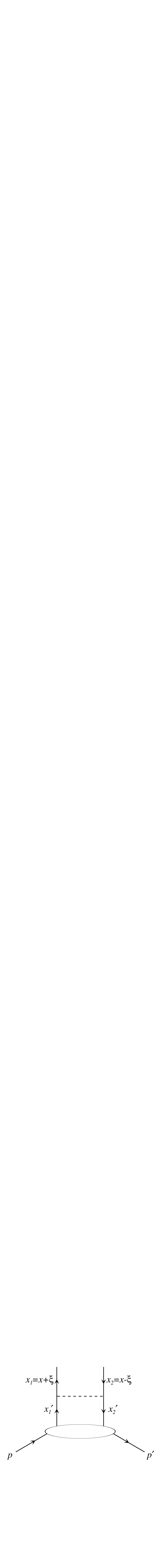
Figure 1: A schematic diagram showing the variables for the off-diagonal parton distribution $H(x,\xi)$ where $x_{1,2}=x\pm\xi$.

with support $-1\leq x\leq 1$ introduced by Ji [1, 2, 3], with the minor difference that the gluon $H_{g}=xH_{g}^{\rm Ji}$. They depend on the momentum fractions $x_{1,2}=x\pm\xi$ carried by the emitted and absorbed partons at each scale $\mu^{2}$ and on the momentum transfer variable $t=(p-p^{\prime})^{2}$, see Fig. 1. The values of $t$ and $\xi=(x_{1}-x_{2})/2$ do not change as we evolve the parton distributions up in the scale $\mu^{2}$. That is $t$ and $\xi$ lie outside the evolution. In the limit $\xi\rightarrow 0$ the distributions reduce to the conventional diagonal distributions

$$H_{q}(x,0) = \left\{\begin{array}[]{c}q(x)\quad\quad\;\;{\rm for}\quad x>0\\ -\bar{q}(-x)\quad{\rm for}\quad x<0\end{array}\right.$$ (3)

$$H_{g}(x,0) = x\>g(x).$$

Detailed reviews of off-diagonal distributions can be found, for example, in refs. [3, 4, 5].

It is usual to anticipate that the $\xi$ dependence of $H$ is controlled by the non-perturbative starting (input) distribution at some low scale $\mu^{2}=Q_{0}^{2}$. However here we wish to explore the possibility that, in the small $x,\xi\ll 1$ region, the “skewed” off-diagonal behaviour comes mainly from the evolution. Indeed we expect this to be the case. At each step of the evolution the momentum fraction carried by parton $i$ ($i=1,2$) decreases. So when the evolution length is sufficiently large (i.e. $\ln(Q^{2}/Q_{0}^{2})\gg 1$), the important values of $x\sim x_{0}$ of the input $(\mu^{2}=Q_{0}^{2}$), which control the behaviour in the $x\sim\xi$ domain at the high scale $(\mu^{2}=Q^{2})$, will satisfy $x_{0}\gg\xi$. Clearly we can neglect the $\xi$ dependence in the $x_{0}$ region and start evolving from purely diagonal partons with $x_{1}=x_{2}$.

Here we demonstrate how, in the phenomenologically important small $\xi$ region (for $t\rightarrow 0$), the off-diagonal distributions are determined unambiguously in terms of the small $x$ behaviour of the (conventional) diagonal partons which is known from experiment. We therefore have the attractive possibility to include data described by off-diagonal distributions in a global parton analysis to better constrain the small $x$ behaviour of the diagonal distributions.

2 Off-diagonal distributions in terms of conformal moments

In terms of the Operator Product Expansion (OPE) the evolution of the off-diagonal distributions may be viewed as the renormalisation of the matrix elements $O_{N}=\langle p^{\prime}|\hat{O}_{N}|p\rangle$ of the conformal (Ohrndorf [6]) operators, where $p$ and $p^{\prime}$ are the momenta of the incoming and outgoing protons. For the quark, the leading twist operator $\hat{O}_{N}$ is of the form

$$\hat{O}_{N}^{q}\;=\;\sum_{k=0}^{N}\>\left(\begin{array}[]{c}N\\ k\end{array}\right)\>\left(\begin{array}[]{c}N+2\\ k+1\end{array}\right)\>\partial_{L}^{k}\>\partial_{R}^{N-k}$$ (5)

where the derivatives $\partial_{L}$ and $\partial_{R}$ act on the left and right quarks in Fig. 1. As a consequence the quark matrix element takes the form

$$O_{N}^{q}\;=\;\int_{-1}^{1}\>dx\>R_{N}^{q}(x_{1},x_{2})\>H_{q}(x,\xi)$$ (6)

with $x_{1,2}=x\pm\xi$, where the polynomials [7]

$$R_{N}^{q}\;=\;\sum_{k=0}^{N}\>\left(\begin{array}[]{c}N\\ k\end{array}\right)\>\left(\begin{array}[]{c}N+2\\ k+1\end{array}\right)\>x_{1}^{k}\>x_{2}^{N-k}.$$ (7)

In other words the polynomials $R_{N}(x_{1},x_{2})$ are the basis which specifies the conformal moments $O_{N}$. In the diagonal limit, with $x_{1}=x_{2}$, (6) reduces to the well-known moments

$$M_{N}^{q}\;=\;\int_{0}^{1}\>x^{N}\>q(x)\>dx.$$ (8)

Unlike the common $x^{N}$ basis in the diagonal case, the gluon and quark polynomial bases differ from each other. For the gluon we have

$$R_{N}^{g}\;=\;\sum_{k=0}^{N}\>\left(\begin{array}[]{c}N\\ k\end{array}\right)\>\left(\begin{array}[]{c}N+4\\ k+2\end{array}\right)\>x_{1}^{k}\>x_{2}^{N-k},$$ (9)

to be compared with the quark polynomials of (7).

Recall that the off-diagonal distributions are symmetric in $\xi$ [2, 3]

$$H_{i}(x,\xi)\;=\;H_{i}(x,-\xi)$$ (10)

with $i=q$ or $g$. This is just the left-right or $x_{1}\leftrightarrow x_{2}$ symmetry of Fig. 1. In terms of the $x$ variable the symmetry relations are

$$H_{q}^{s}(x,\xi) = -H_{q}^{s}(-x,\xi),$$

$$H_{q}^{ns}(x,\xi) = H_{q}^{ns}(-x,\xi),$$ (11)

$$H_{g}(x,\xi) = H_{g}(-x,\xi)$$

for the quark singlet, non-singlet and gluon respectively.

The conformal moments $O_{N}$ have the advantage that they are not mixed, at least at LO, during the off-diagonal evolution, but simply get multiplicatively renormalized

$$O_{N}(Q^{2})\;=\;O_{N}(Q_{0}^{2})\>\left(\frac{Q^{2}}{Q_{0}^{2}}\right)^{\gamma_{N}}$$ (12)

with the same anomalous dimension $\gamma_{N}$ as in the diagonal case. The problem of how to restore the analytic off-diagonal distribution $H(x,\xi)$ from knowledge of its conformal moments $O_{N}(\xi)$ of (6) has been solved recently by Shuvaev [8]. The prescription is as follows. We first calculate an auxiliary function

$$f(x^{\prime},\xi;t)\;\equiv\;f(x^{\prime})\;=\;\int\>\frac{dN}{2\pi i}\>(x^{\prime})^{-N}\>O_{N}(\xi)/R_{N}(1,1)$$ (13)

using a simple Mellin transform, where for simplicity of presentation we shall omit the arguments $\xi,t$ and $\mu^{2}$ of $f$. Next we perform the convolution

$$H(x,\xi)\;=\;\int_{-1}^{1}\>dx^{\prime}\>{\cal K}(x,\xi;x^{\prime})\>f(x^{\prime}),$$ (14)

where, for quarks, the kernel is given by

$${\cal K}_{q}(x,\xi;x^{\prime})\;=\;-\frac{1}{\pi|x^{\prime}|}\>{\rm Im}\>\int_{0}^{1}\>ds(1-y(s)x^{\prime})^{-3/2}$$ (15)

with

$$y(s)\;=\;\frac{4s(1-s)}{x+\xi(1-2s)}.$$ (16)

To gain insight into the Shuvaev prescription we repeat that, from a theoretical OPE point of view, it is best to analyse experimental data for processes described by off-diagonal distributions in terms of the conformal moments $O_{N}$ of (6) which diagonalize the (LO) evolution. However, phenomenologically it is more convenient to work in terms of the off-diagonal parton distributions themselves. The Shuvaev transform (13) and (14) performs the necessary inverse of (6) at any fixed $\xi,t$ and $\mu^{2}$; that is it enables $H(x,\xi)$ to be constructed from $O_{N}(\xi)$. So far this is just a mathematical procedure. The crucial physical step is to relate the auxiliary function $f(x^{\prime})$ directly to the diagonal partons. It is easy to show, for $\xi\ll 1$, that $f(x^{\prime})$ in fact reduces to a diagonal parton distribution. Indeed the conformal moments may be expressed in the form

$$O_{N}(\xi)\;=\;\sum^{[(N+1)/2]}_{k=0}\>O_{Nk}\>\xi^{2k},$$ (17)

which embodies the “polynomial condition” that the power of $\xi$ should be at most of the order of $N+1$. For $\xi\ll 1$ we have

$$O_{N}(\xi)\;\simeq\;O_{N0}\;=\;O_{N}(0).$$ (18)

Now, up to the trivial normalization factor $R_{N}(1,1)$, the diagonal moment $O_{N}(0)$ is equal to the $x^{N}$ moment of the diagonal parton distribution. So for $\xi\ll 1$ we can put $f_{q}(x^{\prime})=q(x^{\prime})$ in (14), and then use (15) to determine the off-diagonal distribution $H_{q}(x,\xi)$ in terms of the conventional quark distribution. In this limit the kernel ${\cal K}$ just becomes a non-trivial representation of the delta function $\delta(x-x^{\prime})$.

Since (15) is a principal value integration, the apparent singularity at $y(s)x^{\prime}=1$ is not a problem. However, for computation purposes, it is convenient to first weaken this singularity in the $s$ integration by integrating by parts. Then (14) and (15) become

$$H_{q}(x,\xi)\;=\;\int_{-1}^{1}\>dx^{\prime}\left[\frac{2}{\pi}\>{\rm Im}\>\int_{0}^{1}\>\frac{ds}{y(s)\>\sqrt{1-y(s)x^{\prime}}}\right]\>\frac{d}{dx^{\prime}}\left(\frac{q(x^{\prime})}{|x^{\prime}|}\right).$$ (19)

Here we have used the properties that $q(x^{\prime})\rightarrow 0$ as $x^{\prime}\rightarrow 1$ and that

$$q^{s}(x^{\prime})\;=\;-q^{s}(-x^{\prime}),\quad\quad q^{ns}(x^{\prime})\;=\;q^{ns}(-x^{\prime}),$$ (20)

see (2). Note that, for small $\xi$, we can identify the auxiliary function $f(x^{\prime})$ of (13) with the diagonal partons at any scale, as the same anomalous dimensions $\gamma_{N}$ control both the diagonal and off-diagonal evolution.

So far we have neglected the $t$ dependence and set $t=0$. However from the sum rule [3] we know that the $t$ dependence of the first conformal moment is given by the proton form factor $G(t)$,

$$O_{N=0}(t)\;=\;\langle p^{\prime}|\hat{O}_{0}|p\rangle\;\propto\;G(t).$$ (21)

In fact it is natural to assume that all the moments are proportional to $G(t)$

$$O_{N}(t)\;=\;O_{N}(t=0)\>G(t)$$ (22)

and simply multiply (14) by $G(t)$ to restore the $t$ dependence of the distributions. Another argument in favour of such a factorization is the form of the Mellin integration (13) where, for small $x$, the saddle point is located near the singularity at $N=0$ which comes from the behaviour of the singlet anomalous dimension, $\gamma_{N}\propto 1/N$. Thus the dominant contribution comes from $O_{N=0}$ which is indeed proportional to $G(t)$, and due to the polynomial condition (17) does not depend on $\xi$ at all [3].

The formula for the gluon is a little different to that for the quarks. The reason is that in the off-diagonal case the functions $H_{q}$ and $H_{g}=xH_{g}^{\rm Ji}$ form the singlet multiplet which is multiplicatively renormalized. The additional $x$ in the gluon reveals itself as an extra factor of $x+\xi(1-2s)$ in the kernel. Thus for the gluon, in place of (19), we have

$$H_{g}(x,\xi;t)\;=\;xH_{g}^{\rm Ji}\;=\;\int_{-1}^{1}\>dx^{\prime}\left[\frac{2}{\pi}\>{\rm Im}\>\int_{0}^{1}\>\frac{ds(x+\xi(1-2s))}{y(s)\>\sqrt{1-y(s)x^{\prime}}}\right]\>\frac{d}{dx^{\prime}}\left(\frac{g(x^{\prime})}{|x^{\prime}|}\right)\>G(t).$$ (23)

3 Predictions of the off-diagonal distributions for small $x$ and $\xi$

We see that (19) and (23) completely determine the behaviour of the off-diagonal distributions in the small $x,\xi$ domain in terms of the diagonal distributions. In fact by making the physically reasonable small $x$ assumption that the diagonal partons are given by

$$xq(x)\;=\;N_{q}\>x^{-\lambda_{q}},\quad\quad xg(x)\;=\;N_{g}\>x^{-\lambda_{g}}$$ (24)

we can perform the $x^{\prime}$ integration analytically. We obtain

$$H_{i}(x,\xi;t)\;=\;N_{i}\>\frac{\Gamma\left(\lambda+\frac{5}{2}\right)}{\Gamma(\lambda+2)}\>\frac{2}{\sqrt{\pi}}\>\int_{0}^{1}\>ds\left[x+\xi(1-2s)\right]^{p}\>\left[\frac{4s(1-s)}{x+\xi(1-2s)}\right]^{\lambda_{i}+1}\>G(t)$$ (25)

with $i=q$ or $g$, and where $p=0$ and 1 for quarks and the gluon respectively.

At first sight it appears that for singlet quarks (where $\lambda_{q}>0$ and $p=0$) we face a strong singularity in integral (25) when the term $D\equiv x+\xi(1-2s)\rightarrow 0$ in the denominator. Fortunately the singlet quark distribution is antisymmetric in $x$. To obtain the imaginary part of the integral (19) we must choose $x^{\prime}>0$ for $D>0$ and $x^{\prime}<0$ for $D<0$. Therefore we must treat (25) as a principal value integral and take the difference between the $D\rightarrow 0+$ and $D\rightarrow 0-$ limits. Thus the main singularity is cancelled and (25) becomes integrable for any $\lambda_{q}<1$.

Note that the dominant contribution to the $x^{\prime}$ integrations of (19) and (23) comes from the region of small $x^{\prime}\sim x,\xi$. Indeed with the input given by (24), the integral for the quark distribution has a strong singularity at small $x^{\prime}$

$$I_{q}\;\sim\;\int\>dx^{\prime}(x^{\prime})^{-\lambda_{q}-3}\>{\rm Im}\left(\frac{1}{y(s)\sqrt{1-y(s)x^{\prime}}}\right).$$ (26)

However when we take the imaginary part, the $x^{\prime}$ integration is cut-off by the theta function $\theta(x^{\prime}-1/y(s))$ at

$$x^{\prime}\;=\;1/y(s)\;\sim\;x+\xi(1-2s).$$ (27)

So we obtain the small $\xi$ behaviour $I_{q}\sim\xi^{-\lambda_{q}-1}$, and the distribution (19) has the form

$$H_{q}(x,\xi)\;=\;\xi^{-\lambda_{q}-1}\>F_{q}(x/\xi).$$ (28)

Similarly it follows that $H_{g}=\xi^{-\lambda_{g}}F_{g}(x/\xi)$.

The predictions for the off-diagonal distributions are shown in Fig. 2. In diagrams (a)–(c) we show the ratio $R$ to the diagonal distribution in the form

$$R\;=\;\frac{H(x,\xi)}{H(x+\xi,0)},$$ (29)

and so the only free parameter is $\lambda$, the exponent which fixes the $x^{-\lambda}$ behaviour of the input diagonal partons, as in (24). Notice that on account of (28) the ratios $R$ at small $x$ and $\xi$ are a function of only the ratio of the variables $x/\xi$.

The ratios $R$ of (29) are the relevant ratios. For example, high energy diffractive $q\bar{q}$ electroproduction is described by two gluon exchange with

$$x_{1}\;\simeq\;(Q^{2}+M_{q\bar{q}}^{2})\>\big{/}\>W^{2}\gg x_{2},$$ (30)

where $W$ is the centre-of-mass energy of the proton and the photon of virtuality $Q^{2}$. A common approximation is to describe the process in terms of the diagonal gluon $x_{1}g(x_{1})$, sampled at $x_{1}=x+\xi$. In this case the inclusion of off-diagonal effects will enhance the cross section by a factor of $R_{g}^{2}$, where $R_{g}$ is evaluated at $x/\xi=1$, see Fig. 2(b) or 2(d).

For $x\gg\xi$ we see that the off-diagonal to diagonal ratios, $R$, tend to unity, as expected. Moreover, due to the $x\rightarrow-x$ antisymmetry property (2), we see that the quark singlet vanishes as $x\rightarrow 0$. Also for a flat input gluon, $xg(x)\rightarrow$ constant as $x\rightarrow 0$ (that is $\lambda_{g}=0$), we see that $R_{g}$ does not depend on $\xi$ at all. The same is true for the quarks, but now when $q(x)\rightarrow$ constant, that is when $\lambda_{q}=-1$, as seen in the $R_{q}^{ns}=1$ result of Fig. 2(c).

All the scale dependence of the distributions is hidden in the $Q^{2}$ behaviour of the powers $\lambda(Q^{2})$. The position of the saddle point $N=\lambda$ in the Mellin integral (13) moves to the right in the complex $N$ plane as $Q^{2}$ and so the off-diagonal “enhancement” increases; in other words $R$ increases with $Q^{2}$. A particular example is the double logarithm approximation when, in the singlet sector, the saddle point

$$N\;=\;\lambda_{g}(Q^{2})\;\simeq\;\sqrt{(\alpha_{S}/\pi)\>\ln(1/x)\>\ln(Q^{2}/Q_{0}^{2})}.$$ (31)

In Fig. 2(d) we show the off-diagonal gluon distribution again, but now using a (more detailed) linear scale and comparing with the diagonal distribution $H(\bar{x},0)$ taken at fixed $\bar{x}=2\xi$, so as to avoid the extra $x$ dependence coming from the diagonal gluon in the denominator of the $R_{g}$ ratio. This demonstrates that the extra $x$ dependence is responsible for the slight decrease observed in $R_{g}$ of Fig. 2(b) as $x\rightarrow 0$, and that the decrease is not due to the behaviour of $H_{g}(x,\xi)$.

The behaviour of the ratios at $x=\xi$ are explicitly

$$R\;=\;\frac{H(\xi,\xi)}{H(2\xi,0)}\;=\;\frac{2^{2\lambda+3}}{\sqrt{\pi}}\frac{\Gamma(\lambda+5/2)}{\Gamma(\lambda+3+p)}\,,$$

where $p=0$ for quarks and $p=1$ for gluons. The ratios are plotted in Fig. 3 as a function of $\lambda$. The vertical arrows shown on the plot indicate the values of $\lambda_{g}$ and $\lambda_{q}$ obtained from the gluon and sea quark distributions at $Q^{2}=4$ and 100 GeV² of a recent global (diagonal) parton analysis [9]. The plot can be used to find the enhancement of the cross section for the high energy diffractive electroproduction of vector mesons arising from off-diagonal parton effects. The enhancement is given by $R_{g}^{2}$ where $R_{g}$ is the value of the gluon ratio at $x=\xi$, which is shown in Fig. 3, at the appropriate scale, that is at the appropriate value of $\lambda_{g}(Q^{2})$. For instance, for the photoproduction of $J/\psi$ and $\Upsilon$ at HERA the enhancement is about (1.15)² and (1.32)² respectively, if we use a scale $M_{V}^{2}/4$, where $M_{V}$ is the mass of the vector meson.

From Figs. 2 and 3 we see that the off-diagonal or “skewed” effect (the ratio $R$) is much stronger for singlet quarks than for gluons. The explanation is straightforward. At low $x$ the distributions are driven by the double leading logarithmic evolution of the gluon distribution. At each step of the evolution the momentum fractions $x_{i}$ are strongly ordered ($x_{1}^{\prime}\gg x_{1},x_{2}^{\prime}\gg x_{2}$ on Fig. 1). For gluons it is just the “last splitting function” $P_{gg}(x_{2},x_{2}^{\prime};\xi)$ which generates the main $\xi$ dependence, or skewedness, of the distribution. However for the sea or singlet quarks it is necessary to produce a quark with the help of $P_{qg}$ at the last splitting. The splitting function $P_{qg}$ has no logarithmic $1/z=x_{2}^{\prime}/x_{2}$ singularity and so $x_{2}$ is the order of $x_{2}^{\prime}$. Consequently both the splitting functions $P_{qg}(x_{2},x_{2}^{\prime};\xi)$ and $P_{gg}(x_{2}^{\prime},x_{2}^{\prime\prime};\xi)$ generate the asymmetry of the off-diagonal distribution. Hence, at low $x$, the singlet quark has a much stronger off-diagonal effect than the gluon.

4 Discussion

In order to conclude that the conformal moments allow us to use the diagonal partons to uniquely determine the off-diagonal partons at small $x$ and $\xi$, including also their normalisation and $Q^{2}$ behaviour, it is necessary to consider some further points.

First we could worry that in the analytical continuation in $N$ of the conformal moments,

$$O_{N}\;=\;\sum_{k}\>\xi^{2k}\>O_{Nk}\quad\quad{\rm with}\quad\quad 2k\><\>N+1,$$ (32)

the higher ($k\geq 1$) terms will generate a singularity at $N>\lambda+2k$. In such a case the small $x,\xi$ contribution would be driven by this singularity. However we show that such a singularity to the right of $N=\lambda+2k$ cannot occur. From the structure of the polynomials $R_{N}(x_{1},x_{2})$ of (7) and (9), it is clear that there are no such singularities for integer $N>2k$. On the other hand a singularity at non-integer $N=\beta+2k$ would generate a function $f(x^{\prime})$ of (13) which depends on the ratio $\xi^{2k}/x^{\prime\beta+2k}$. After the convolution (14) we would obtain a distribution which violates the polynomial condition [3],

$$\int\>dx\>x^{N}\>H(x,\xi)\;=\;\sum_{k=0}^{[(N+1)/2]}\>A_{k}\xi^{2k},$$ (33)

which comes from Lorentz invariance (and the tensor structure of the operators). Thus the higher $\xi^{2}$ terms (with $k\geq 1$) in (17) should die out with decreasing $\xi$.

A second consideration is that, from a formal point of view, we may add to the off-diagonal distribution any function

$$\Delta H(x,\xi)\;=\;g(x,\xi)\>\theta(\xi-|x|)$$ (34)

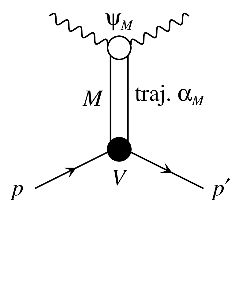
Figure 4: Meson ($M$) Regge exchange indicating the structure of the off-diagonal contribution of (35).

which exists only in the time-like ERBL region [12] with $|x|<\xi$. Such a contribution $\Delta H$ remains in the ERBL region during evolution. However $\Delta H$ disappears as $\xi\rightarrow 0$ and so it cannot be restored purely from diagonal partons. A physical way to model such an ERBL contribution is to consider $t$ channel meson ($M$) exchanges of Fig. 4. The contribution $\Delta H$ is then given by the leading twist wave function $\psi_{M}$ of the meson multiplied by the corresponding Regge exchange amplitude

$$\Delta H^{\rm Reggeon}\;=\;\psi_{M}(x/\xi,Q^{2})\xi^{-\alpha_{M}(t)}\>V(\mu^{2}=Q_{0}^{2};\xi;t).$$ (35)

The appropriate exchange is the $f_{2}$ meson which, in the constituent quark model, is formed from a $P$-wave $q\bar{q}$ state with $J^{PC}=2^{++}$. The Regge factor $\xi^{-\alpha_{M}}$ is the analogue of the $x^{-\eta}$ (or $\xi^{-\eta}$) factor in the non-singlet quark distribution $H^{ns}\sim x^{-\eta}$; in our notation of (24) and Fig. 2 with $xq^{ns}\sim x^{-\lambda_{ns}}$ we have $\lambda_{ns}=\eta-1$. Phenomenologically we expect that $\eta\sim\alpha_{M}(0)\sim 0.5$. The key factor in (35) is $V$ which specifies the coupling of the Reggeon to the proton. From Regge phenomenology the vertex factor $V$ was extracted for the diagonal case where the ERBL domain does not exist. Let us try to estimate a possible ERBL contribution to the off-diagonal distributions. The value of the pion-nucleon $\Sigma$-term at low scales determines the number of current quarks and antiquarks in the nucleon to be [13]

$$\langle N|\bar{q}q|N\rangle\;\simeq\;8.$$ (36)

Allowing for valence quarks, this implies that the average number of $q\bar{q}$ pairs is about 2.5. At such low scales the partons are distributed more or less uniformly in the whole $(-1,1)$ interval and so the probability to find two partons in the ERBL domain $(-\xi,\xi)$ is of the order of $\xi^{2}$. Such a $\Delta H$ is a negligible $O(\xi^{2})$ contribution at small $\xi$ in agreement with our decomposition of the conformal moments.

So far our distributions enable us to calculate the imaginary part of the amplitude, say for Compton scattering with incoming and outgoing photon virtualities $q^{2}=-Q^{2}$ and $q^{\prime 2}=-Q^{\prime 2}$. At small $x$ and $\xi$ it turns out that the real part of the amplitude may be calculated easily using a dispersion relation in the centre-of-mass energy squared $W_{s}^{2}=(p+q)^{2}$. Let us consider the cut in the right-half $W_{s}$ plane, that is the discontinuity for $W_{s}^{2}>0$. For fixed $t,Q^{2}$ and $Q^{\prime 2}$, the ratio $r=x/\xi$ is fixed as well, since $(x+\xi)/(x-\xi)=Q^{2}/Q^{\prime 2}$. Thus the energy squared may be written

$$W_{s}^{2}\;=\;(1-x)\>\frac{Q^{2}}{x+\xi}\;=\;(1-r\xi)\>\frac{Q^{2}}{1+r}\>\frac{1}{\xi}.$$ (37)

However we must take into account the cuts in both right and left half-planes, that is the $s$ and $u$ channel cuts. The left-hand cut corresponds to the $u$ channel process (obtained by the interchange $p\leftrightarrow-p^{\prime}$) with energy squared

$$W_{u}^{2}\;=\;-(1+x)\>\frac{Q^{2}}{x+\xi}.$$ (38)

The unpolarized deeply virtual Compton amplitude is the sum of the $s$- and $u$- channel terms, $A=A_{s}+A_{u}$, and appears to have even signature, that is $A$ is crossing symmetric. Strictly speaking at large $x$ and $\xi$ there is some asymmetry (since $W_{u}^{2}\neq-W_{s}^{2}$), which may be considered as the odd signature contribution and should be treated appropriately in the dispersion integral. However the situation is particularly simple at small $x\ll 1$, where $(1\pm x)\simeq 1$. Then we may write the whole amplitude $A\propto(W^{2})^{\lambda}$, with the help of the even signature factor

$${\cal S}^{+}\;=\;\frac{1}{2}(1+(-1)^{\lambda}),$$ (39)

in the form

$$A\;=\;\frac{i}{2}\>{\rm Im}A(1+e^{-i\pi\lambda}).$$ (40)

Moreover for small $\lambda$ we have

$${\rm Re}A\;\simeq\;\frac{\pi\lambda}{2}\>{\rm Im}A.$$ (41)

Strictly speaking the conformal moments $O_{N}$ only renormalize multiplicatively, as in (12), at leading order (LO). Due to a conformal anomaly at next-to-leading (NLO) the moment $O_{N}$ mixes, on evolution, with moments $O_{N^{\prime}}$ with $N^{\prime}<N$ [14]. The mixing is taken into account by a matrix $\mbox{\boldmath$B$}_{NN^{\prime}}$, which obeys its own evolution equation [15]. Of course the mixing is absent in the diagonal case when $\xi\rightarrow 0$, whereas for non-zero $\xi$ we have

$$O_{N}^{\rm NLO}\;=\;\sum_{N^{\prime}=0}^{N}\>\mbox{\boldmath$B$}_{NN^{\prime}}\>O_{N^{\prime}}^{\rm NLO(diag)}\>\xi^{N-N^{\prime}}$$ (42)

where $O_{N},O_{N^{\prime}}$ and $\mbox{\boldmath$B$}_{NN^{\prime}}$ all depend on $\alpha_{S}(Q^{2})$. Thus in the small $\xi\ll 1$ limit we can safely use expressions (19) and (23) for $H(x,\xi)$ even at NLO.

In summary, in the low $\xi$ region we can use expressions (19) and (23) to reliably predict the off-diagonal distributions $H(x,\xi)$ in terms of the diagonal partons at any scale. All that is required is a two-fold integration. The expected accuracy is of the order of $\xi^{2}$. As a specific example we assumed in (24) that the diagonal partons had a power-like $x^{-\lambda}$ behaviour for small $x$. In this case one integration can be done analytically and we have even simpler expressions for $H_{q}$ and $H_{g}$, see (25). The results are shown in Figs. 2 and 3 and allow the off-diagonal distributions to be determined for any small $x,\xi$ values at any scale. One important consequence is that data for processes, which are described by off-diagonal distributions, can be included in a global analysis to better constrain the low $x$ behaviour of the (conventional) diagonal partons.

Acknowledgements

We thank Lev Lipatov for helpful discussions. This work was supported in part by the Royal Society, INTAS (95-311), the Russian Fund for Fundamental Research (98 02 17629), the Polish State Committee for Scientific Research grant No. 2 P03B 089 13 and by the EU Fourth Framework Programme TMR, Network ‘QCD and the Deep Structure of Elementary Particles’ contract FMRX-CT98-0194 (DG12-MIKT) and (DG12-MIHT).

Figure 2: Predictions at small $x$ and $\xi$ for the ratio of off-diagonal ($H(x,\xi)$) to diagonal $(H_{q}(\bar{x},0)=f_{q}(\bar{x}),H_{g}(\bar{x},0)=\bar{x}f_{g}(\bar{x}))$ parton distributions. The diagonal partons are taken to have the form $xf(x)=Nx^{-\lambda}$. Plots (a), (b) and (c) show the quark singlet, gluon and quark non-singlet ratios taking $\bar{x}=x+\xi$ as the argument of the diagonal partons. Plot (d) shows the gluon ratio again but versus a linear scale and with argument $\bar{x}=2\xi$ so as to display the $x$ behaviour of $H_{g}(x,\xi)$.

Figure 3: The off-diagonal to diagonal ratio, $R$, at small $x$ and $\xi$ versus the power $\lambda$ which specifies the $x^{-\lambda}$ behaviour of the input diagonal parton as in (24). Note that the quark singlet ratio has been divided by 2. The vertical arrows indicate the values of $\lambda$ found in a global parton analysis [9] at $Q^{2}=4$ and 100 GeV².

References

- [1] X. Ji, Phys. Rev. Lett. 78 (1997) 610.
- [2] X. Ji, Phys. Rev. D55 (1997) 7114.
- [3] X. Ji, J. Phys. G24 (1998) 1181.
- [4] A.V. Radyushkin, Phys. Rev. D56 (1997) 5524.
- [5] K.J. Golec-Biernat and A.D. Martin, Phys. Rev. D59 (1999) 014029.
- [6] Th. Ohrndorf, Nucl. Phys. B198 (1982) 26.
- [7] A.P. Bukhvostov, G.V. Frolov, L.N. Lipatov and E.A. Kuraev, Nucl. Phys. B258 (1985) 601.
- [8] A. Shuvaev, hep-ph/9902318.
- [9] A.D. Martin, R.G. Roberts, W.J. Stirling and R.S. Thorne, Eur. Phys. J. C4 (1998) 463.
- [10] A.D. Martin and M.G. Ryskin, Phys. Rev. D57 (1998) 6692.
- [11] A.D. Martin, M.G. Ryskin and T. Teubner, hep-ph/9901420.
-
[12]
A.V. Efremov and A.V. Radyuskin, Phys. Lett. B94 (1980) 245;
S.J. Brodsky and G.P. Lepage, Phys. Lett. B87 (1979) 359. -
[13]
See, for example, J. Gasser, M. Leutwyler and M.E. Sainio,
Phys. Lett. B253 (1991) 252;
J. Gasser and H. Leutwyler, Phys. Rep. 87 (1982) 154. -
[14]
S.J. Brodsky et al., Phys. Rev. D33 (1986) 1881,
D. Müller, Phys. Rev. D49 (1994) 2525. -
[15]
A.V. Belitsky, D. Müller, L. Niedermeier and A. Schäfer,
hep-ph/9810275;
A.V. Belitsky and D. Müller, Nucl. Phys. B537 (1999) 397; and references therein.