HARD-PHOTON EMISSION IN $e^{+}e^{-}\to{\bar{f}}f$ WITH REALISTIC CUTS

We derive compact analytical formulae of the Bonneau-Martin type for the reaction $e^{+}e^{-}\to{\bar{f}}f\gamma$ with cuts on minimal energy and acollinearity of the fermions, where the photons may be emitted both from the initial or final states. Soft-photon exponentiation is also taken into account.

One of the cleanest scattering processes at elementary particle accelerators is fermion-pair production in $e^{+}e^{-}$ annihilation, potentially accompanied by one or few photons:

$$e^{+}e^{-}\to{\bar{f}}f+(n)\gamma.$$ (1)

Initial-state corrections may be written as an integral over the (normalized) invariant mass squared $R=s^{\prime}/s$ of the final-state fermion pair:

$$\sigma_{T}^{ini}(s)=\int dR~{}\sigma^{0}(s^{\prime})~{}\rho_{T}^{ini}(R),$$ (2)

where $\sigma^{0}(s^{\prime})$ is an effective Born cross-section. The radiator function $\rho_{T}^{ini}(R)$ for the initial-state first-order corrections to the total cross-section $\sigma_{T}$, with soft-photon exponentiation, is [?]:

$$\rho_{T}^{ini}(R) = \left(1+{\bar{S}}\right)\beta(1-R)^{\beta-1}+{\bar{H}}_{T}^{ini}(R),$$ (3)

with

$${\bar{S}} = \frac{3}{4}\beta+\frac{\alpha}{\pi}Q_{e}^{2}\left(\frac{\pi^{2}}{3}-\frac{1}{2}\right)+h.o.,~{}~{}~{}~{}~{}\beta=\frac{2\alpha}{\pi}Q_{e}^{2}\left(\ln\frac{s}{m_{e}^{2}}-1\right),$$ (4)

and

$${\bar{H}}_{T}^{ini}(R) = \left[H_{BM}(R)-\frac{\beta}{1-R}\right]+h.o.,$$ (5)

where $h.o.$ stands for higher orders, and [?]:

$$H_{BM}(R)=\frac{1}{2}~{}\frac{1+R^{2}}{1-R}~{}\beta.$$ (6)

Experiments at LEP1, SLC, LEP2, and those planned at a linear collider aim at precisions well below a per cent and need theoretical predictions with an accuracy of the order of 0.1 % or better. A basic ingredient of the predictions is the complete photonic $O(\alpha)$ correction including initial and final state radiations and their interferences:

$$\sigma(s) = \sigma^{0}(s)+\sigma^{ini}(s)+\sigma^{int}(s)+\sigma^{fin}(s).$$ (7)

These corrections have to be determined for two basic quantities: The total cross-section $\sigma_{T}(s)$ and the forward-backward asymmetry $A_{FB}=\sigma_{F-B}/\sigma_{T}$; other asymmetries may then easily be derived.

Basically, there are two experimental set-up’s to be treated:

• a lower cut on $s^{\prime}$, $s^{\prime}_{min}\geq 4m_{f}^{2}$, often applied to quark-pair production;

• combined cuts on acollinearity $\xi$, $\xi_{max}\leq 180^{\circ}$, and minimal energy $E_{min}$, $E_{min}\geq m_{f}$, of the fermions; often applied to lepton-pair production.

Both cut settings may be combined with an acceptance cut $c$, $c\leq 1$, on the cosine of the fermionic production angle $\cos\theta$.

For case (i), a generalization of the Bonneau-Martin formula, including the complete first-order photonic corrections together with soft-photon exponentiation, may be found in [?] without and in [?] with acceptance cut. The extremely compact expressions for case (i) with $c=1$ get quite more involved when the acceptance cut is applied.

In this article, we give the complete first-order photonic corrections together with soft-photon exponentiation for case (ii).

A three-fold analytical integration of the squared matrix elements is performed in order to get the integrand of the last one, the $s^{\prime}$-integration over $R$, which is assumed to be performed numerically. One may use the phase-space parameterization derived in [?]. The kinematical regions of two variables are shown in figure 1: the (normalized) invariant mass $x$ of (photon + anti-fermion) in their rest system, and $R$ as introduced above. The first and third analytical integrations are over the full production angle of the photon, $\phi_{\gamma}$, in the (photon + fermion) rest system, and over the cosine of the anti-fermion in the center-of-mass system, $\cos\vartheta$. Both angles are completely independent of $x$ and $R$. As figure 1 shows, we have to determine radiators $\rho_{B}^{b}$ ($B=T,F$–$B$ and $b=ini,int,fin$) in three phase-space regions:

$$\sigma_{B}^{b}(s)=\left[\int_{\mathrm{I}}+\int_{\mathrm{II}}-\int_{\mathrm{III}}\right]~{}d\phi_{\gamma}~{}dx~{}ds^{\prime}~{}d\cos\vartheta\frac{d\sigma_{B}^{b}(A)}{d\phi_{\gamma}dxds^{\prime}d\cos\vartheta},$$ (8)

Region I applies to the simple $s^{\prime}$-cut. The integration over $R$ extends from $R_{min}$ to 1,

$$R_{min} = R_{E}\left(1-\frac{\sin^{2}(\xi_{max}/2)}{1-R_{E}\cos^{2}(\xi_{max}/2)}\right).$$ (9)

In each of the three regions, the boundaries for the integration over $x$ are, for a given value of $R$:

$$x_{max,min} = \frac{1}{2}(1-R)~{}(1\pm A),$$ (10)

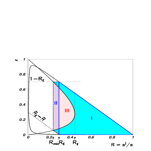
Figure 1: Phase space with cuts on acollinearity and (lower) fermion energy.

where the parameter $A=A(R)$ depends in every region on only one of the cuts applied:

$$A_{\mathrm{I}} = \sqrt{1-\frac{R_{m}}{R}},$$ (11)

$$A_{\mathrm{II}} = \frac{1+R-2R_{E}}{1-R},$$ (12)

$$A_{\mathrm{III}} = \sqrt{1-\frac{R(1-R_{\xi})^{2}}{R_{\xi}(1-R)^{2}}},$$ (13)

with:

$$R_{m} = \frac{4m_{f}^{2}}{s},$$ (14)

$$R_{E} = \frac{2E_{min}}{\sqrt{s}},$$ (15)

$$R_{\xi} = \frac{1-\sin(\xi_{max}/2)}{1+\sin(\xi_{max}/2)}.$$ (16)

Initial State Radiation

Here, for $\sigma_{T}^{ini}(s)$ the Bonneau-Martin function gets replaced by:

$$H_{T}^{ini}(R,A) = \frac{3\alpha}{4\pi}Q_{e}^{2}\left[\left(A+\frac{A^{3}}{3}\right)\frac{1+R^{2}}{1-R}\left(\ln\frac{s}{m_{e}^{2}}-1\right)+(A-A^{3})\frac{2R}{1-R}\right].$$ (17)

In $\sigma_{F-B}^{ini}(s)$, the corresponding hard radiator part is:

$$H^{ini}_{F-B}(R;A\geq A_{0}) = \frac{\alpha}{\pi}Q_{e}^{2}\Biggl{\{}\frac{1+R^{2}}{1-R}\Biggl{[}\frac{4R}{(1+R)^{2}}\left(\ln\frac{s(1+R)^{2}}{4m_{e}^{2}R}-1\right)$$ (18)

$$-~{}\frac{1}{(1+R)^{2}}\left[y_{+}y_{-}\ln\left|y_{+}y_{-}\right|+{4R}\ln(4R)\right]$$

$$-~{}(1-A^{2})\left(\ln\frac{s}{4m_{e}^{2}(1+A)^{2}R}-1\right)\Biggr{]}+\frac{4A(1-A)R}{1-R}\Biggr{\}},$$

$$H^{ini}_{F-B}(R;A<A_{0}) = \frac{\alpha}{\pi}Q_{e}^{2}\Biggl{\{}\frac{1+R^{2}}{1-R}\left[-\frac{y_{+}y_{-}}{(1+R)^{2}}\ln\left|\frac{y_{+}}{y_{-}}\right|+(1-A^{2})\ln\frac{1+A}{1-A}\right]$$ (19)

$$+~{}\frac{8AR^{2}}{(1+R)(1-R)}\Biggr{\}}.$$

These functions have to be used in (3) and its analogue, with equal ${\bar{S}}$, for $\sigma_{F-B}^{ini}$. The following definitions are used:

$$A_{0} = \frac{1-R}{1+R},$$ (20)

$$y_{\pm} = (1-R)\pm A(1+R).$$ (21)

In region I, the above expressions (17) and (18) reduce to those known from [?] and [?]. In this region the radiators diverge for $R\to 1$, and soft-photon exponentiation and the subtraction $\beta/(1-R)$ is applied there (and only there) in order to get ${\bar{H}}_{B}^{ini}(R)$; see (5).

Initial-Final State Interferences

In the initial-final state interferences, the effective Born cross-sections depend on both $s$ and $s^{\prime}$ as well as on the type of exchanged vector particles $V_{i}$ (e.g. photon and or $Z$):

$$\sigma_{B}^{int}(s) = \int dR\sum_{V_{i},V_{j}=\gamma,Z}\sigma_{\bar{B}}^{0}(s,s^{\prime},i,j)~{}\rho_{B}^{int}(R,A,i,j).$$ (22)

For $B$=$T$ it is ${\bar{B}}$=$F$–$B$ and vice versa. We give as examples simple model-independent Born expressions in order to fix the overall normalization:

$$\sigma_{T}^{0}(s,s^{\prime}) = \sum_{V_{i},V_{j}=\gamma,Z}\sigma_{T}^{0}(s,s^{\prime},i,j)=\frac{4\pi\alpha^{2}}{3s^{\prime}}~{}{\cal V},$$ (23)

$$\sigma_{F-B}^{0}(s,s^{\prime}) = \sum_{V_{i},V_{j}=\gamma,Z}\sigma_{F-B}^{0}(s,s^{\prime},i,j)=\frac{\pi\alpha^{2}}{s^{\prime}}~{}{\cal A},$$ (24)

with

$${\cal V} = Q_{e}^{2}Q_{f}^{2}+|Q_{e}Q_{f}|v_{e}v_{f}\Re e[\chi(s)+\chi(s^{\prime})]+(v_{e}^{2}+a_{e}^{2})(v_{f}^{2}+a_{f}^{2})\Re e[\chi(s)\chi^{*}(s^{\prime})],$$ (25)

$${\cal A} = |Q_{e}Q_{f}|a_{e}a_{f}\Re e[\chi(s)+\chi(s^{\prime})]+4v_{e}a_{e}v_{f}a_{f}\Re e[\chi(s)\chi^{*}(s^{\prime})],$$ (26)

and with the following $Z$ boson propagators:

$$\chi(s) = \frac{G_{\mu}M_{Z}^{2}}{8\sqrt{2}\pi\alpha}\frac{s}{s-M_{Z}^{2}+iM_{Z}\Gamma_{Z}}.$$ (27)

The radiator functions are:

$$\rho_{B}^{int}(R,A;i,j) = \delta(1-R)\left[S_{B}+b_{B}(i,j)\right]+\theta(1-R-\epsilon)H_{B}^{int}(R,A).$$ (28)

The box contributions $b_{T}(i,j)$ may be taken from equations (116) and (118) (to be multiplied by 4/3) of [?] and the $b_{F-B}(i,j)$ from equations (123) and (126). For convenience, we give the soft corrections explicitly:

$$S_{T}^{int} = 8\frac{\alpha}{\pi}Q_{e}Q_{f}\left(1-\ln\frac{2\epsilon}{\lambda}\right),$$ (29)

$$S_{F-B}^{int} = \frac{\alpha}{\pi}Q_{e}Q_{f}\left[-\left(1+8\ln 2\right)\ln\frac{2\epsilon}{\lambda}+4\ln^{2}2+\ln 2+\frac{1}{2}+\frac{1}{3}\pi^{2}\right].$$ (30)

Finally, the hard radiator parts are:

$$H^{int}_{T}(R,A) = -\frac{\alpha}{\pi}Q_{e}Q_{f}\frac{4AR(1+R)}{1-R},$$ (31)

and

$$H^{int}_{F-B}(R,A\geq A_{0}) = \frac{\alpha}{\pi}Q_{e}Q_{f}\Biggl{\{}\frac{3R}{2}\left[\ln\frac{z_{+}}{z_{-}}+\frac{2-R+\frac{5}{3}R^{2}}{1-R}\ln R\right]$$ (32)

$$-~{}\frac{1+R}{2(1-R)}(5-2R+5R^{2})\ln\frac{(1+R)(1+A)}{2}$$

$$+~{}\frac{1}{4(1-R)}\Biggl{[}\frac{(1-4R+R^{2})[A(1+R)^{2}-(1-R)^{2}]}{1+R}$$

$$+~{}2A(1-A)(1+R^{3})\Biggr{]}\Biggr{\}},$$

$$H^{int}_{F-B}(R,A<A_{0}) = \frac{3\alpha}{2\pi}Q_{e}Q_{f}~{}R\Biggl{\{}\ln\frac{z_{+}}{z_{-}}-\frac{2-R+\frac{5}{3}R^{2}}{1-R}\ln\frac{1+A}{1-A}+A(1-R)\Biggr{\}},$$ (33)

with

$$z_{\pm} = (1+R)\pm A(1-R).$$ (34)

Again, for $A\to 1$ the $H^{int}_{T}(R,A)$ and $H^{int}_{F-B}(R,A\geq A_{0})$ approach the known expressions of the $s^{\prime}$ cut given in [?].

Final State Radiation

The final state corrections to order $O(\alpha)$ are:

$$\sigma_{B}^{fin}(s) = \sigma_{B}^{0}(s)\int dR~{}\rho_{B}^{fin}(R,A),$$ (35)

with

$$\rho_{B}^{fin}(R,A) = \delta(1-R)S_{f}+\theta(1-R-\epsilon)H_{B}^{fin}(R,s,A),$$ (36)

$$S_{f} = {\bar{S}}_{f}+\beta_{f}\ln\epsilon,$$ (37)

where ${\bar{S}}_{f}$ and $\beta_{f}$ are the final state’s analogues of ${\bar{S}}$ and $\beta$. The hard radiators are:

$$H^{fin}_{T}(R,s,A) = \frac{\alpha}{\pi}Q_{f}^{2}\left[\frac{1+R^{2}}{1-R}\ln\frac{1+A}{1-A}-\frac{8Am_{f}^{2}/s}{(1-A^{2})(1-R)}-A(1-R)\right],$$ (38)

$$H^{fin}_{F-B}(R,s,A) = H^{fin}_{T}(R,A)+\frac{\alpha}{\pi}Q_{f}^{2}\left[A(1-R)-(1+R)\ln\frac{z_{+}}{z_{-}}\right].$$ (39)

Common initial- and final state soft-photon exponentiation may be performed as follows [?,?]:

$$\sigma_{B}^{ini+fin}(s) = \int dR~{}\sigma^{0}(s^{\prime})~{}\rho_{B}^{ini}(R,A)~{}{\bar{\rho}}_{B}^{fin}(R,s^{\prime},A),$$ (40)

with

$${\bar{\rho}}_{B}^{fin}(R,s^{\prime},A)=(1-R_{E})^{\beta^{\prime}_{f}}(1+S^{\prime}_{f})+\int_{R_{min}/R}^{1}du\left[H^{fin}_{B}(u,s^{\prime},A^{\prime})-\frac{\beta^{\prime}_{f}}{1-u}\theta(R-R_{E})\right].$$ (41)

The soft part of $\rho_{B}^{fin}(u,s^{\prime},A^{\prime})$, $A^{\prime}=A(u)$, and $\beta^{\prime}_{f}$ are derived from (3) by replacing there $Q_{e}$ by $Q_{f}$ and $s/m_{e}^{2}$ by $s^{\prime}/m_{f}^{2}$. We mention here that in the hard radiators the integration over $u$ may also be performed analytically. In region III, one has to interchange for this the order of integration over $u$ and $x$ [?].

Conclusions

We recalculated the photonic corrections with acollinearity cut having applications in the Fortan program ZFITTER in mind [?]. When the code was created in 1989 [?], an accuracy of 0.5 % at LEP1 was assumed to be needed .

We performed several numerical applications of the above formulae. For this purpose, the package acol.f was added. As a result, we conclude that ZFITTER until version 5.20 treats the $O(\alpha)$ photonic corrections with acollinearity cut with a numerical accuracy for $\sigma_{T}$ of not less than about 0.4 % near the $Z$ resonance (LEP1 energy region, $\sqrt{s}$ within $M_{Z}\pm 3$ GeV) or better (at resonance). The coding with acol.f gave a numerical agreement of $\sigma_{T}$ for leptons, with $\xi_{max}\leq 10^{\circ}$ and $E_{min}=1$ GeV, with predictions from TOPAZ0 v.4.4 [?] at LEP1 of 0.01 % (at the wings) or better (at resonance) [?]. For $A_{FB}$, we estimate at LEP1 energies the accuracy of the $O(\alpha)$ photonic corrections with acollinearity cut in ZFITTER until v.5.20 to be about 0.02 % or better at the resonance and about 0.13 % or better at the wings. The numerical limitations at LEP1 are due to the initial-final state interference.

For applications at higher energies, the accuracy of ZFITTER with acollinearity cut was not dedicatedly controlled until recently, although there was reason to suspect that it comes out much worse than at LEP1. With the cuts mentioned, the accuracy of v.5.20 at LEP2 is again limited by the initial-final interference but not less than roughly 1 %.

A higher accuracy in the acollinearity mode is prevented in ZFITTER until v.5.20 by several reasons. The main reason is a neglect of a certain class of ordinary, angular dependent $O(\alpha)$ terms in the initial state and in the initial-final state interference hard radiator parts. Some numerical approximations in the treatment of final state radiation may also be influential; this has not been studied in detail so far.

Finally we should like to mention that the correct $O(\alpha)$ hard radiators for the angular distributions and for the integrated cross-sections with cuts on both acollinearity and angular acceptance also have been determined within this project and will be published elsewhere together with a scetch of the calculations and more numerical results.

Acknowledgments

We would like to thank D. Bardin, S. Vasileva, M. Grünewald, G. Passarino, and S. Riemann for numerical comparisons, and D. Bardin for a careful discussion of the conclusions.

References

References

• [1] M. Greco, G. Pancheri-Srivastava, and Y. Srivastava, Nucl. Phys. B101 (1975) 234–262.
• [2] G. Bonneau and F. Martin, Nucl. Phys. B27 (1971) 381–397.
• [3] D. Bardin, M. Bilenky, A. Chizhov, A. Sazonov, Y. Sedykh, T. Riemann, and M. Sachwitz, Phys. Lett. B229 (1989) 405.
• [4] D. Bardin, M. Bilenky, A. Sazonov, Y. Sedykh, T. Riemann, and M. Sachwitz, Phys. Lett. B255 (1991) 290–296.
• [5] G. Passarino, Nucl. Phys. B204 (1982) 237–266.
• [6] D. Bardin, M. Bilenky, A. Chizhov, A. Sazonov, O. Fedorenko, T. Riemann, and M. Sachwitz, Nucl. Phys. B351 (1991) 1–48.
• [7] O. Nicrosini and L. Trentadue, Z. Physik C39 (1988) 479.
• [8] G. Montagna, O. Nicrosini, and G. Passarino, Phys. Lett. B309 (1993) 436–442.
• [9] D. Bardin et al., Fortran program ZFITTER v.4.6, CERN-TH. 6443/92 (1992), hep-ph/9412201; v.5.20 (17 Feb 1999) and many earlier versions are available from /afs/ cern.ch/user/b/bardindy/public and http://www.ifh.de/~riemann/Zfitter/zf.html.
• [10] M. Bilenky and A. Sazonov, ZFITTER Fortran routines for photonic corrections with acollinearity and acceptance cuts, unpublished (1989).
• [11] P. Christova, M. Jack, S. Riemann, and T. Riemann, “Predictions for fermion-pair production at LEP”, DESY 98-184 (1998), to appear in the proceedings of RADCOR 98, Sep 8-12, 1998, Barcelona, Spain, hep-ph/9812412.
• [12] D. Bardin, M. Grünewald, and G. Passarino, “Precision Calculation Project Report”, hep-ph/9902452.
• [13] G. Montagna et al., Fortran program TOPAZ0 v.4.0, FNT/T 98/02 (1998), hep-ph/9804211, v.4.4 available from http://www.to.infn.it/~giampier/topaz0.html.
• [14] D. Bardin, M. Grünewald, and G. Passarino, TOPAZ0 values by private communication.