LPT–Orsay–98–83 NORDITA–99–11–HE SPbU–IP–99–04 hep-ph/9902375

Baryon Distribution Amplitudes in QCD

V.M. Braun¹, S.É. Derkachov², G.P. Korchemsky³ and A.N. Manashov⁴

¹NORDITA, Blegdamsvej 17, DK-2100 Copenhagen, Denmark

² Department of Mathematics, St.-Petersburg Technology Institute,
St.-Petersburg, Russia

³ Laboratoire de Physique Théorique, Université de Paris XI,
91405 Orsay Cédex, France

⁴ Department of Theoretical Physics, Sankt-Petersburg State University,
St.-Petersburg, Russia

Abstract:
We develop a new theoretical framework for the description of leading twist light-cone baryon distribution amplitudes which is based on integrability of the helicity $\lambda=3/2$ evolution equation to leading logarithmic accuracy. A physical interpretation is that one can identify a new ‘hidden’ quantum number which distinguishes components in the $\lambda=3/2$ distribution amplitudes with different scale dependence. The solution of the corresponding evolution equation is reduced to a simple three-term recurrence relation. The exact analytic solution is found for the component with the lowest anomalous dimension for all moments $N$, and the WKB-type expansion is constructed for other levels, which becomes asymptotically exact at large $N$. Evolution equations for the $\lambda=1/2$ distribution amplitudes (e.g. for the nucleon) are studied as well. We find that the two lowest anomalous dimensions for the $\lambda=1/2$ operators (one for each parity) are separated from the rest of the spectrum by a finite ‘mass gap’. These special states can be interpreted as scalar diquarks.

1 Introduction

There exists a general consensus that exclusive processes involving large momentum transfers are dominated by ‘valence’ components in hadron wave functions with the minimum number of Fock constituents [1, 2]. It is equally generally accepted that the asymptotic behavior of exclusive amplitudes is in most cases determined by the so-called ‘hard-rescattering’ mechanism involving configurations of partons with almost zero transverse separations, although the theoretical status of the dominance of small transverse distances is somewhat weaker for baryons [3] than for pions [4, 5].

As always in a field theory, extraction of the asymptotic behavior introduces divergences. In the present context, infrared divergences in perturbative diagrams describing the hard rescattering are removed by renormalization of nonperturbative scale-dependent distribution amplitudes which are defined in terms of the Bethe-Salpeter wave functions integrating out transverse degrees of freedom

$$\phi(x_{1},\ldots,x_{n};\mu)\sim\int\limits^{|k_{i,\perp}|<\mu}\!\!\!d^{2}k_{1,\perp}\ldots d^{2}k_{n,\perp}\,\Phi_{BS}(x_{1},k_{1,\perp};\ldots;x_{n},k_{n,\perp})$$ (1.1)

with $x_{i}$ being the longitudinal momentum fractions carried by partons. The concept of distribution amplitudes is central for the theory of hard exclusive processes where their rôle is analogous to that of more familiar parton distributions in the description of inclusive processes.

The theoretical basis for studies of distribution amplitudes [4] is provided by their definition in terms of hadron-to-vacuum transition matrix elements of non-local gauge-invariant light-cone operators of the type (in a suitably chosen gauge)

$$\bar{q}(z_{1}n)q(z_{2}n),$$

$$\varepsilon_{ijk}q^{i}(z_{1}n)q^{j}(z_{2}n)q^{k}(z_{3}n)$$ (1.2)

for meson and baryon distributions, respectively. Here $q^{i}$ is a generic quark field with the color $i$, $n$ is an auxiliary light-like vector $n^{2}=0$ and $z_{i}$ are real numbers that specify quark (antiquark) separations. More specific definitions will be given below. The nonlocal operators as above are understood as generating functionals for the series of local operators obtained by their Tailor expansion at short distances (contraction of the derivatives with the light-like vector ensures taking the leading twist part) and the precise relation is such that moments of distribution amplitudes are given by matrix elements of the contributing local operators [4]. The scale dependence of the moments of distribution amplitudes corresponds to the renormalization group (RG) evolution of local operators and can be studied using familiar methods.

The specific problem for distribution amplitudes is to take into account the additional mixing with operators containing total derivatives that cannot be neglected in contrast to inclusive processes where only forward matrix elements are being considered. It was noticed that the RG evolution is driven to leading logarithmic accuracy by tree-level counterterms which thus have the symmetry of the bare QCD Lagrangian and, in particular, the conformal symmetry. As a consequence, operators belonging to different irreducible representations of the conformal group cannot mix under renormalization in one loop [4, 6, 7, 8, 9]. This observation solves the mixing problem for meson (two-particle) distributions in which case a single independent local conformal operator exists for each moment. The corresponding anomalous dimension can be continued analytically to non-integer (complex) moments, defining the Altarelli-Parisi evolution kernel: coefficients in the expansion of meson distributions in the basis of Gegenbauer polynomials are renormalized multiplicatively and with the same anomalous dimensions as in deep inelastic scattering [4]. Consequently, assuming ‘good’ behavior at complex infinities, the distribution amplitude can be restored by inverse Mellin transform from analytically continued values of the moments; hence the partonic interpretation of the distribution amplitude proves to be consistent with its renormalization properties (scale dependence).

The three-quark baryon distribution amplitudes bring in a complication of principle. The conformal symmetry allows to resolve the mixing with total derivatives but is not sufficient to diagonalize the mixing matrix completely. For fixed operator dimension, alias for fixed total number $N$ of covariant derivatives, $D_{\mu}=\partial_{\mu}-igA_{\mu}$, there exist $N+1$ independent local operators (modulo operators with the total derivatives)

$${\cal O}_{N,k}=q\,(\stackrel{{\scriptstyle\leftarrow}}{{D}}\cdot n)^{k}q\,(n\cdot\!\stackrel{{\scriptstyle\rightarrow}}{{D}})^{N-k}q,~{}~{}~{}k=0,\ldots,N$$ (1.3)

corresponding to $N+1$ genuine independent degrees of freedom of the three-quark system. One is left with a nontrivial $(N+1)\times(N+1)$ mixing matrix that has to be diagonalized explicitly order by order; see, e.g., [10, 11, 12, 8, 13, 14]. The resulting $N+1$ multiplicatively renormalizable operators have different (in general) anomalous dimensions whose analytic expressions are not known. Apart from mathematical incompleteness, absence of analytic results means that the general structure of the spectrum is unknown and, in particular, analytic continuation of the anomalous dimensions to complex moments $N$ is not possible. This, in turn, implies that partonic interpretation of different ‘components’ in baryons is not understood beyond the tree level.

This problem was well known but considered as a relatively minor one and did not attract due attention in the past. One reason was that the scale dependence of distribution amplitudes turned out to be rather mild in a perturbative domain and it seemed premature to elaborate on the evolution before gross features of nonperturbative distributions were understood at low scales. We think that this logic is flawed and the general experience with hard processes in QCD rather suggests that ‘intrinsic’ parton distributions at scales of order 1 GeV cannot be viewed as purely nonperturbative and disconnected from perturbative evolution. Despite an obvious fact that perturbative calculations cannot be made quantitative at low scales, there is increasing evidence that general patterns of the perturbative gluon emission are continued to very low momenta. For example, the shape of deep inelastic structure functions at 1 GeV appears to be largely determined by perturbative soft gluon radiation. Small differences in the perturbative evolution of different components in nucleon distribution amplitudes are strongly amplified in the nonperturbative domain and one may think that such differences build up gross features of distribution amplitudes at scales of order 1 GeV, where from the perturbation theory becomes quantitative. Viewed from this perspective, a detailed study of the evolution of baryon distribution amplitudes becomes mandatory.

In this paper we suggest a new approach to the construction of baryon distribution amplitudes which is based on the recent finding [15] that the evolution equation for the baryon distribution amplitudes with maximum helicity $\lambda=3/2$ is completely integrable. That is it possesses a nontrivial integral of motion which we identify as a new ‘hidden’ quantum number that distinguishes components in the $\lambda=3/2$ distribution amplitudes with different scale dependence. It is interesting to note that the $\lambda=3/2$ evolution equation is equivalent to the quantum mechanical problem that has already been encountered in QCD in the studies of the Regge asymptotics of the scattering amplitudes [16, 17] and in the theory of integrable models as the so-called Heisenberg XXX_s=-1 spin magnet [16, 18]. This problem has been studied in some detail using nontrivial mathematical methods and the results can be adapted to the present context.

Our approach is advantageous compared to the standard formulation in at least two aspects. First, from practical point of view an important simplification is that diagonalization of a $(N+1)\times(N+1)$ matrix is replaced by solution of a simple three-term recurrence relation, which reduces the computer time significantly. Second, we obtain explicit analytic solutions to the evolution equations in all important limits. In particular, we will be able to identify trajectories of the anomalous dimensions and calculate them (and the corresponding eigenfunctions) using a WKB type expansion for large values of $N$.

These results apply in full to the $\lambda=3/2$ distribution function of the $\Delta$-resonance and allow for a fairly complete description. The evolution equation for the $\lambda=1/2$ distributions is not exactly solvable, but the difference to the $\lambda=3/2$ evolution can be considered as a small (calculable) perturbation for the most part of the spectrum. On the other hand, the structure of the lowest eigenstates is changed drastically. As we will demonstrate, the two lowest anomalous dimensions for the $\lambda=1/2$ operators decouple from the rest of the spectrum and are separated from it by a finite ‘mass gap’. These two special states (one for each parity) can be interpreted as bound states in the corresponding quantum-mechanical model, and, somewhat imprecisely, can be thought of as corresponding to formation of scalar diquarks.

As a byproduct of our study, we construct a convenient orthonormal basis for the expansion of three-particle distribution amplitudes, which is more suitable compared to standard Appell polynomials.

The presentation is organized as follows. Section 2 introduces definitions and the general framework for the construction of baryon distribution functions and their renormalization. Section 3 is devoted to the conformal symmetry of the evolution equation and the conformal expansion of distribution amplitudes. Section 4 presents a detailed study of the exactly solvable evolution equation for the maximum helicity $\lambda=3/2$. In Section 5 we consider the evolution equation for the $\lambda=1/2$ distributions. A short summary of main results of phenomenological relevance is given in Section 6 and the general conclusions in Section 7. Appendix A presents an explicit construction for the Racah $6j-$coefficients of the $SL(2)$ group and in Appendix B we consider the effective Hamiltonian for low-frequency modes of the $\lambda=1/2$ evolution equation.

2 General framework

2.1 Distribution amplitudes

Following Refs. [19] we define the leading twist nucleon distribution amplitude as the corresponding matrix element of the gauge-invariant three-quark nonlocal operator

$$\langle 0|u_{\alpha}^{i^{\prime}}(z_{1})u_{\beta}^{j^{\prime}}(z_{2})d_{\gamma}^{k^{\prime}}(z_{3})\,U_{i^{\prime}i}(z_{1},z_{0})U_{j^{\prime}j}(z_{2},z_{0})U_{k^{\prime}k}(z_{3},z_{0})\epsilon^{ijk}|P(p,\lambda)\rangle=$$

$$=\frac{f_{N}}{4}\left\{(\not\!pC)_{\alpha\beta}(\gamma_{5}N)_{\gamma}V(z_{i}p)+(\not\!p\gamma_{5}C)_{\alpha\beta}N_{\gamma}A(z_{i}p)+\left(i\sigma_{\mu\nu}p^{\nu}C\right)_{\alpha\beta}(\gamma_{\mu}\gamma_{5}N)_{\gamma}T(z_{i}p)\right\},$$

where $\sigma_{\mu\nu}=\frac{i}{2}[\gamma_{\mu},\gamma_{\nu}]$, $C$ is the charge conjugation matrix, $|P(p,\lambda)\rangle$ is the proton state with momentum $p$ and helicity $\lambda$, and $N$ is the proton spinor. All the interquark separations are assumed to be light-like, e.g. $u(z_{1})$ denotes the u-quark field at the space point $z_{1}n$ with $n^{2}=0$, and $U(z_{n},z_{0})$ are non-Abelian phase factors (light-like Wilson lines)

$$U(z_{n},z_{0})\equiv{\rm P\ exp\,}\left[ig\int_{0}^{1}\!dt\,(z_{n}-z_{0})\,n_{\mu}A^{\mu}(tz_{n}+(1-t)z_{0})\right].$$ (2.2)

Because of the light-cone kinematics, the matrix element in fact does not depend on $z_{0}$ and the phase factors can be eliminated by choosing a suitable gauge. To save space we do not show the gauge phase factors in what follows, but imply that they are always present.

The invariant functions $V,A,T$ have the following symmetry properties [19]

$$V(1,2,3)=V(2,1,3),\ \ \ \ A(1,2,3)=-A(2,1,3),\ \ \ \ \ T(1,2,3)=T(2,1,3).$$ (2.3)

and can be expressed in terms of a single function $\phi_{N}$ as

$$2T(1,2,3) = \phi_{N}(1,3,2)+\phi_{N}(2,3,1),$$

$$\phi_{N}(1,2,3) = V(1,2,3)-A(1,2,3).$$ (2.4)

Here $\phi_{N}$ is the leading twist proton distribution amplitude. If it is presented in the form

$$\phi_{N}(z_{i}p)\equiv\int\!{\cal D}x\,\exp\Big{[}-i\sum x_{i}z_{i}(p\cdot n)\Big{]}\phi_{N}(x_{i}),$$ (2.5)

where

$$\int\!{\cal D}x\equiv\int_{0}^{1}\!dx_{1}\,dx_{2}\,dx_{3}\,\delta(1-x_{1}-x_{2}-x_{3}),$$ (2.6)

then the variables $x_{i}$ have the meaning of the longitudinal momentum fractions carried by the three quarks in the nucleon, $0\leq x_{i}\leq 1$ and $\sum x_{i}=1$.

For what follows, it is convenient to introduce quark fields with definite chirality

$$q^{\uparrow(\downarrow)}=\frac{1}{2}\left(1\pm\gamma_{5}\right)q.$$ (2.7)

The definition in (2.1) is equivalent to the following form of the proton state [19, 20]

$$|P(p,\lambda=+1/2)\rangle=f_{N}\int\frac{{\cal D}x\,\phi_{N}(x)}{2\sqrt{24x_{1}x_{2}x_{3}}}\left\{|u^{\uparrow}(x_{1})u^{\downarrow}(x_{2})d^{\uparrow}(x_{3})\rangle-|u^{\uparrow}(x_{1})d^{\downarrow}(x_{2})u^{\uparrow}(x_{3})\rangle\right\},$$ (2.8)

where the standard relativistic normalization for the states and Dirac spinors is implied [21]. The distribution amplitude $\phi_{N}$ can be defined in terms of chiral fields:

$$\langle 0|\epsilon^{ijk}(u_{i}^{\uparrow}(z_{1})\,C\!\!\not\!nu_{j}^{\downarrow}(z_{2}))\not\!nd_{k}^{\uparrow}(z_{3})|P(p)\rangle=$$ (2.9)

$${}\hskip 14.22636pt=-\frac{1}{2}f_{N}(pn)\not\!nN^{\uparrow}(p)\int\!{\cal D}x\,\exp\big{[}-ipn(z_{1}x_{1}+z_{2}x_{2}+z_{3}x_{3})\big{]}\,\phi_{N}(x_{i},\mu^{2})$$

so that moments of $\phi_{N}$

$$\phi_{N}(k_{1},k_{2},k_{3})=\int\!{\cal D}x\,x_{1}^{k_{1}}x_{2}^{k_{2}}x_{3}^{k_{3}}\,\phi_{N}(x_{1},x_{2},x_{3},\mu^{2})$$ (2.10)

can be calculated as reduced matrix elements of the renormalized three-quark leading twist operators

$$O_{k_{1},k_{2},k_{3}}^{\uparrow\downarrow\uparrow}=(nD)^{k_{1}}u^{\uparrow}(0)(C\!\not\!n)(nD)^{k_{2}}u^{\downarrow}(0)(nD)^{k_{3}}\not\!nd^{\uparrow}(0),$$ (2.11)

where $D_{\mu}=\partial_{\mu}-igA_{\mu}$ is a covariant derivative.

The leading twist distribution amplitudes of the $\Delta$ resonance can be obtained in the similar manner [20]. For definiteness, we will consider the distribution amplitudes of $\Delta^{++}$ only, all the other ones can be reconstructed with the help of the isospin symmetry, see [20]. For this case one writes

$$\langle 0|u_{\alpha}^{i}(z_{1})u_{\beta}^{j}(z_{2})u_{\gamma}^{k}(z_{3})|\Delta^{++}(p,\lambda)\rangle\epsilon^{ijk}=$$ (2.12)

$$=\frac{\lambda^{1/2}_{\Delta}}{4}\left\{(\gamma_{\mu}C)_{\alpha\beta}(\Delta)^{\mu}_{\gamma}V_{\Delta}(z_{i}p)+(\gamma_{\mu}\gamma_{5}C)_{\alpha\beta}(\gamma_{5}\Delta^{\mu})_{\gamma}A_{\Delta}(z_{i}p)\right.$$

$$-\left.\frac{1}{2}\left(i\sigma_{\mu\nu}C\right)_{\alpha\beta}(\gamma_{\mu}\Delta^{\nu})_{\gamma}T_{\Delta}(z_{i}p)\right\}-\frac{1}{4}f_{\Delta}^{3/2}\left(i\sigma_{\mu\nu}C\right)_{\alpha\beta}\left(p_{\mu}\Delta^{\nu}-\frac{1}{2}M_{\Delta}\gamma_{\mu}\Delta^{\nu}\right)_{\gamma}\phi_{\Delta}^{3/2}(z_{i}p).$$

Here $\Delta_{\gamma}^{\mu}(p)$ is the $\Delta$ resonance spin$-\frac{3}{2}$ vector:

$$(\not\!p-M_{\Delta})\Delta^{\mu}=0,\ \ \ \bar{\Delta}^{\mu}\Delta_{\mu}=-2M_{\Delta},\ \ \ \gamma_{\mu}\Delta^{\mu}(p)=p_{\mu}\Delta^{\mu}(p)=0.$$ (2.13)

The dimensionless amplitudes $V_{\Delta}(x),A_{\Delta}(x),T_{\Delta}(x)$ determine the distribution of quarks in the $\Delta(|\lambda|=1/2)$ state and satisfy the following symmetry relations

$$V_{\Delta}(1,2,3) = V_{\Delta}(2,1,3),\ \ \ \ A_{\Delta}(1,2,3)=-A_{\Delta}(2,1,3),$$

$$T_{\Delta}(1,2,3) = T_{\Delta}(2,1,3),$$ (2.14)

$$T_{\Delta}(1,2,3) = V_{\Delta}(2,3,1)-A_{\Delta}(2,3,1).$$

Therefore, only one function is independent; we choose (cf. [20])

$$\phi_{\Delta}^{1/2}(x_{1},x_{2},x_{3})\equiv V_{\Delta}(x_{1},x_{2},x_{3})-A_{\Delta}(x_{1},x_{2},x_{3})=T_{\Delta}(x_{3},x_{1},x_{2})$$ (2.15)

as the distribution amplitude of the $\Delta(|\lambda|=1/2)$ resonance. The remaining function $\phi_{\Delta}^{3/2}$ is totally symmetric in all its arguments and determines the distribution of quarks in the $\Delta(|\lambda|=3/2)$ state.

The structure, again, becomes more transparent when going over to chiral quark fields. The definition in Eq. (2.1) is equivalent to the following structure of the $\Delta$ resonance states [20]

$$|\Delta(\lambda=1/2)\rangle = f_{\Delta}^{1/2}\int{\cal D}x\frac{\phi_{\Delta}^{1/2}(x_{i})}{4\sqrt{24x_{1}x_{2}x_{3}}}|u^{\uparrow}(x_{1})u^{\downarrow}(x_{2})u^{\uparrow}(x_{3})\rangle,$$

$$|\Delta(\lambda=3/2)\rangle = f_{\Delta}^{3/2}\int{\cal D}x\frac{\phi_{\Delta}^{3/2}(x_{i})}{6\sqrt{24x_{1}x_{2}x_{3}}}|u^{\uparrow}(x_{1})u^{\uparrow}(x_{2})u^{\uparrow}(x_{3})\rangle,$$ (2.16)

where $f_{\Delta}^{3/2}=\sqrt{\frac{2}{3}}\lambda_{\Delta}^{1/2}/M_{\Delta}$, and the distribution amplitudes can be defined through the nonlocal matrix elements:

$$\langle 0|\epsilon^{ijk}(u_{i}^{\uparrow}(z_{1})\,C\!\!\not\!nu_{j}^{\downarrow}(z_{2}))\not\!nu_{k}^{\uparrow}(z_{3})|\Delta(p)\rangle=$$ (2.17)

$${}=-\frac{1}{2}\lambda_{\Delta}^{1/2}n^{\mu}(\!\not\!n\Delta)^{\uparrow}_{\mu}\int\!{\cal D}x\,\exp\big{[}-ipn(z_{1}x_{1}+z_{2}x_{2}+z_{3}x_{3})\big{]}\,\phi_{\Delta}^{1/2}(x_{i},\mu^{2})$$

and

$$\langle 0|\epsilon^{ijk}(u_{i}^{\uparrow}(z_{1})\,C\sigma_{\mu\nu}n_{\nu}u_{j}^{\uparrow}(z_{2}))(\bar{\Delta}^{\mu}\!\!\not\!n)\,u_{k}^{\uparrow}(z_{3})|\Delta(p)\rangle=$$ (2.18)

$${}={i}\,f_{\Delta}^{3/2}(pn)\bar{\Delta}^{\uparrow}_{\nu}\!\not\!n\Delta^{\uparrow,\nu}\int\!{\cal D}x\,\exp\big{[}-ipn(z_{1}x_{1}+z_{2}x_{2}+z_{3}x_{3})\big{]}\,\phi_{\Delta}^{3/2}(x_{i},\mu^{2}).$$

2.2 Renormalization

In this paper we will be interested in the scale dependence of the baryon distribution amplitudes. For each of them, $\phi\equiv\phi_{N},\phi_{\Delta}^{3/2},\phi_{\Delta}^{1/2}$, we anticipate an expansion of the type

$$\phi(x_{i},\mu^{2})=x_{1}x_{2}x_{3}\sum_{n}\phi_{n}\,P_{n}(x_{i})\left(\frac{\alpha_{s}(\mu)}{\alpha_{s}(\mu_{0})}\right)^{\gamma_{n}/b_{0}},$$ (2.19)

where $b_{0}=11/3N_{c}-2/3n_{f}$, $P_{n}(x_{i})$ are certain polynomials, $\gamma_{n}$ are the corresponding anomalous dimensions and $\phi_{n}(\mu_{0})$ are dimensionless nonperturbative parameters. The prefactor $x_{1}x_{2}x_{3}$ suggests the vanishing of the distribution amplitude at the end points $x_{k}=0$ and as we will show its presence is closely related to the conformal invariance of the evolution equations. Finding $\gamma_{n}$ and $P_{n}$ corresponds to explicit diagonalization of the mixing matrix of the three-quark composite operators and is fully equivalent to the solution of the corresponding Brodsky-Lepage equations [3].

Renormalization properties of the relevant three-quark operators are most conveniently presented in terms of their generating functionals (nonlocal operators) with three spinor indices [22]:

$$B^{3/2}_{\alpha\beta\gamma}(z_{1},z_{2},z_{3}) = \varepsilon^{ijk}(\!\not\!nq_{i}^{\uparrow})_{\alpha}(z_{1}n)(\!\not\!nq_{j}^{\uparrow})_{\beta}(z_{2}n)(\!\not\!nq_{k}^{\uparrow})_{\gamma}(z_{3}n),$$ (2.20)

$$B^{1/2}_{\alpha\beta\gamma}(z_{1},z_{2},z_{3}) = \varepsilon^{ijk}(\!\not\!nq_{i}^{\uparrow})_{\alpha}(z_{1}n)(\!\not\!nq_{j}^{\downarrow})_{\beta}(z_{2}n)(\!\not\!nq_{k}^{\uparrow})_{\gamma}(z_{3}n),$$ (2.21)

with $q_{i}$ being a quark field of color $i$. $B_{3/2}$ gives rise to the distribution amplitude $\phi_{\Delta}^{3/2}$ and $B_{1/2}$ is relevant both for $\phi_{N}^{1/2}$ and $\phi_{\Delta}^{1/2}$. The nonlocal operators $B_{3/2}$ and $B_{1/2}$ do not mix with each other since they belong to different representations of the Lorentz group: $(3/2,0)$ and $(1,1/2)$, respectively. For most of the discussion we will assume that all three quarks $q$ have different flavor. Identity of the quarks does not influence renormalization but rather introduces certain selection rules which pick up the eigenstates with particular symmetry, to be detailed later.

The renormalization group equation for the nonlocal operators (2.20), (2.21) can be written as [23, 22]

$$\left\{\mu\,\frac{\partial}{\partial\mu}+\beta(g)\,\frac{\partial}{\partial g}\right\}B={\mathbb{H}}\cdot B,$$ (2.22)

where ${\mathbb{H}}$ is some integral operator corresponding, to the one-loop accuracy, to contributions of the Feynman diagrams shown in Fig. 1.

Figure 1: Examples of a ‘vertex’ correction (a), ’exchange’ diagram (b) and self-energy insertion (c) contributing to the renormalization of three-quark operators in Feynman gauge. Path-ordered gauge factors are shown by the dashed lines. The set of all diagrams includes possible permutations.

To simplify notations, we factor out the color factors and trivial contributions of the self-energy insertions:

$${\mathbb{H}}=(1+1/N_{c}){\cal H}+3C_{F}/2,$$ (2.23)

with $C_{F}=(N_{c}^{2}-1)/(2N_{c})$. It is easy to see that the gluon exchange diagram in Fig. 1b vanishes unless the participating quarks have opposite chirality. The renormalization of the $\lambda=3/2$ operator $B_{3/2}$ (2.20) is therefore determined by the vertex correction in Fig. 1a alone (in Feynman gauge). By explicit calculation one finds [10, 23, 11, 12, 13]

$${\cal H}_{3/2}={\cal H}_{12}^{v}+{\cal H}_{23}^{v}+{\cal H}_{13}^{v},$$ (2.24)

where ${\cal H}_{ik}^{v}$ are the two-particle kernels involving the $i$-th and $k$-th quarks, for example,

$${\cal H}_{12}^{v}\,B(z_{i}) = -\int_{0}^{1}\frac{d\alpha}{\alpha}\Big{\{}{\bar{\alpha}}\left[B(z_{12}^{\alpha},z_{2},z_{3})-B(z_{1},z_{2},z_{3})\right]$$ (2.25)

$${}\hskip 28.45274pt+{\bar{\alpha}}\!\left[B(z_{1},z_{21}^{\alpha},z_{3})-B(z_{1},z_{2},z_{3})\right]\!\Big{\}},$$

with $\bar{\alpha}\equiv 1-\alpha$ and $z_{ik}^{\alpha}\equiv z_{i}\bar{\alpha}+z_{k}\alpha$.

In the case of $B_{1/2}$ the vertex correction remains the same, but one has to add contributions of gluon exchange between the quarks with opposite chirality. One obtains

$${\cal H}_{1/2}={\cal H}_{3/2}-{\cal H}_{12}^{e}-{\cal H}_{23}^{e},$$ (2.26)

where we assume that the first and the third quark have the same chirality, as in (2.21). The kernels $H^{e}_{ik}$ act on $i$-th and $k$-th arguments of the nonlocal operators only, and can be written in the form

$${\cal H}_{12}^{e}\,B(z_{i})=\int\!{\cal D}\alpha\,B(z_{12}^{\alpha_{1}},z_{21}^{\alpha_{2}},z_{3})\,,$$ (2.27)

with the integration measure ${\cal D}\alpha$ defined in (2.6).

Going over to local operators corresponds to the Taylor expansion of the generating functionals at small distances:

$$B(z_{1},z_{2},z_{3})=\sum_{N}\sum_{k_{1}+k_{2}+k_{3}=N}\frac{z_{1}^{k_{1}}}{k_{1}!}\frac{z_{2}^{k_{2}}}{k_{2}!}\frac{z_{3}^{k_{3}}}{k_{3}!}(nD)^{k_{1}}q(0)(nD)^{k_{2}}q(0)(nD)^{k_{3}}q(0).$$ (2.28)

The total number of derivatives $N$ is preserved by the evolution so that the integro-differential equation (2.22) takes the matrix form, with the square matrix of size $N(N+1)/2$ for each given $N$ subsector.

A generic local operator with $N$ derivatives can be written as sum of monomials entering the expansion (2.28) with arbitrary coefficients

$${\cal O}=\sum_{k_{1}+k_{2}+k_{3}=N}c_{k_{1},k_{2},k_{3}}(nD)^{k_{1}}q(0)(nD)^{k_{2}}q(0)(nD)^{k_{3}}q(0),$$ (2.29)

and can be represented by a polynomial in three variables

$${\Psi(x_{1},x_{2},x_{3})}=\sum_{k_{1}+k_{2}+k_{3}=N}c_{k_{1}k_{2}k_{3}}x_{1}^{k_{1}}x_{2}^{k_{2}}x_{3}^{k_{3}}.$$ (2.30)

In what follows we refer to $\Psi(x_{i})$ as coefficient function of a local operator. To justify the name, note that $\Psi(x_{i})$ serves as a projector separating the contribution of the local operator $O_{\Psi}$ to the nonlocal operator $B(z_{i})$, which can be made explicit by writing

$${\cal O}_{\Psi}=\Psi(\partial_{1},\partial_{2},\partial_{3})B(z_{1},z_{2},z_{3})|_{z_{i}=0}.$$ (2.31)

Local operators having the same number of derivatives all mix together so that the size of the mixing matrix for given $N$ is $N(N+1)/2$. Since a local operator is completely determined by its coefficient function, diagonalization of the mixing matrix for operators can be reformulated as diagonalization of the mixing matrix for the coefficient functions. Requiring that ${\cal O}_{\Psi}$ (2.31) is multiplicatively renormalized, one ends up with a matrix equation in the space of homogeneous polynomials of degree $N$ of three variables

$${\cal H}\cdot\Psi_{N,q}={\cal E}_{N,q}\Psi_{N,q}\,,$$ (2.32)

whose eigenvalues correspond to the anomalous dimensions

$$\gamma_{N,q}\equiv(1+1/N_{c})\,{\cal E}_{N,q}+3/2\,C_{F}.$$ (2.33)

Note that the eigenfunctions and the eigenvalues have two indices: $N$ which refers to the degree of polynomial alias the total number of derivatives, and $q$ which enumerates the energy levels. In the case of ${\cal H}_{3/2}$ we will later identify $q$ with a conserved charge. The $SL(2)$ symmetry of the equation (2.32) (see below) implies that the anomalous dimensions take real quantized values and the corresponding eigenfunctions are mutually orthogonal with the weight function $x_{1}x_{2}x_{3}$

$$\int{\cal D}x\,x_{1}x_{2}x_{3}\,\Psi_{N,q}(x_{i})\Psi_{N,q^{\prime}}(x_{i})\sim\delta_{q,q^{\prime}}\,.$$ (2.34)

The same property allows to identify the eigenfunctions as the polynomials entering the expansion of the distribution amplitudes in (2.19)

$$P_{n}(x_{i})\equiv\Psi_{N,q}(x_{i}).$$ (2.35)

To see this, consider the matrix element $\langle 0|{\cal O}_{\Psi}|B\rangle=\Psi(\partial_{1},\partial_{2},\partial_{3})\langle 0|B(z_{1},z_{2},z_{3})|B\rangle|_{z_{i}=0}$ and use the representation similar to (2.18) to get

$$\langle 0|{\cal O}_{\Psi}|B(p)\rangle \sim \int\!{\cal D}x\,\left[\Psi(\partial_{1},\partial_{2},\partial_{3})\,{\rm e}^{-ipn(z_{1}x_{1}+z_{2}x_{2}+z_{3}x_{3})}\right]_{z_{i}=0}\,\phi_{B}(x_{i},\mu^{2})$$ (2.36)

$$= (-ipn)^{N}\int\!{\cal D}x\,\Psi(x_{1},x_{2},x_{3})\,\phi_{B}(x_{i},\mu^{2}).$$

Substituting the expansion (2.19) into this relation and taking into account that the operator $O_{\Psi}$ is renormalized multiplicatively (by construction), one immediately finds that, first, the polynomials $P_{n}$ have to coincide with $\Psi_{N,q}$ up to arbitrary normalization and, second, the nonperturbative coefficient $\phi_{n}$ is given by the reduced matrix element of the operator ${\cal O}_{\Psi}$.

Note that the ‘Hamiltonians’ ${\cal H}_{3/2}$ and ${\cal H}_{1/2}$ acting in the space of coefficient functions in (2.32) are not the same as those acting on nonlocal operators, although they are related, of course, and the precise connection can easily be established. Explicit expressions for ${\cal H}_{3/2}$ and ${\cal H}_{1/2}$ in the matrix representation can be found in [10, 12, 8, 13].

3 Conformal invariance

The Lagrangian of massless QCD is known to be invariant under conformal transformations. This symmetry survives for evolution equations at one-loop level since breaking of the conformal Ward identities induced by the nonzero trace of the stress-energy tensor is proportional to the QCD $\beta$ function and is of order $\alpha_{s}^{2}$ [8, 9]. One should expect, therefore, that the evolution operator ${\cal H}$ introduced in the previous section has the same symmetry and in particular commutes with the generators of the conformal group. This property imposes strong constraints on a possible form of the eigenfunctions: In a generic situation the eigenfunctions of two-particle operators are uniquely determined by conformal invariance whereas for three-particle operators one is left with an arbitrary function of one variable. Aim of this section is to work out the necessary framework.

3.1 Collinear subgroup ${\it SL}(2,{\mathbb{R}})$ of the conformal group

Algebra of the full conformal group contains the generators of dilatations $\bf{D}$ and special conformal transformations ${\bf K}_{\mu}$ in addition to the Poincare generators ${\bf P}_{\mu}$ and ${\bf M}_{\mu\nu}$. The algebra reads

$$[{\bf D},{\bf K}_{\mu}]=i{\bf K}_{\mu},~{}~{}~{}[{\bf K}_{\mu},{\bf P}_{\nu}]=-2i(g_{\mu\nu}{\bf D}+{\bf M}_{\mu\nu}),~{}~{}~{}[{\bf D},{\bf M}_{\mu\nu}]=0,$$

$$[{\bf D},{\bf P}_{\mu}]=-i{\bf P}_{\mu},~{}~{}~{}[{\bf K}_{\rho},{\bf M}_{\mu\nu}]=i(g_{\rho\mu}{\bf K}_{\nu}-g_{\rho\nu}{\bf K}_{\mu}),~{}~{}~{}[{\bf K}_{\mu},{\bf K}_{\nu}]=0,$$ (3.1)

plus usual relations for Poincare generators. Action of these generators on an arbitrary quantum field $\Phi$ (e.g. quark or gluon) is given by (see, e.g. [24, 8])

$$\left[{\bf P}_{\mu},\Phi(z)\right]=-i\partial_{\mu}\Phi(z),\ \ \ \ \left[{\bf M}_{\mu\nu}\,,\Phi(z)\right]=\left[i(z_{\nu}\partial_{\mu}-z_{\mu}\partial_{\nu})-{\bf\Sigma}_{\mu\nu}\right]\Phi(z),$$

$$\left[{\bf D},\Phi(z)\right]=-i(z^{\nu}\partial_{\nu}+l)\Phi(z)\,,$$

$$\left[{\bf K}_{\mu},\Phi(z)\right]=-i\left(2z_{\mu}z^{\nu}\partial_{\nu}-z^{2}\partial_{\mu}+2lz_{\mu}-2iz^{\nu}{\bf\Sigma}_{\mu\nu}\right)\Phi(z)\,.$$ (3.2)

Here $l$ is the canonical dimension of $\Phi$ ($l=3/2$ for quarks) and ${\bf\Sigma}_{\mu\nu}$ stands for the spin part of the angular momentum operator. For a quark field $\Phi(z)\equiv q(z)$

$${\bf\Sigma}_{\mu\nu}q\equiv-\frac{1}{2}\sigma_{\mu\nu}q.$$ (3.3)

In this paper we will be interested in the conformal transformations for the fields ‘living’ on the light-cone

$$\Phi(z)\equiv\Phi(zn_{\mu})\,,\qquad n^{2}=0\,.$$ (3.4)

One can check that the only remaining nontrivial generators are ${\bf P}_{+},\>{\bf D},\>{\bf M}_{+-}$ and ${\bf K}_{-}$, where ‘$+$’ and ‘$-$’ stand for the projection on $n_{\mu}$ and on the alternative light-like vector $\bar{n}$, $\bar{n}n=1$, respectively. We will further assume that the field $\Phi$ is chosen to be an eigenstate of the spin operator $\Sigma_{-+}$, that is it has fixed spin projection $s$ on the ‘+’ direction

$$\Sigma_{-+}\,\Phi=i\,s\,\Phi.$$ (3.5)

For the leading-twist quark operators (2.20), (2.21) $s=+1/2$ for each of the three quarks since $\Sigma_{-+}(\!\not\!nq)=+i(\!\not\!nq)/2$.

To bring the commutation relations (3.1) to the standard form it is convenient to consider the following linear combinations:

$${\bf L}_{+} = {\bf L}_{1}-i{\bf L}_{2}=\frac{i}{2}{\bf K}_{-},\ \ \ \ \ \ \ {\bf L}_{-}={\bf L}_{1}+i{\bf L}_{2}=-i{\bf P}_{+},$$

$${\bf L}_{0} = \frac{i}{2}({\bf D}+{\bf M}_{-+}),\ \ \ \ \ \ \ {\bf E}=\frac{i}{2}({\bf D}-{\bf M}_{-+}).$$ (3.6)

The operators ${\bf L}_{i}$ form the so-called collinear subalgebra $SL(2,{\mathbb{R}})$ of the conformal algebra:

$$\left[{\bf L}_{+},{\bf L}_{-}\right]=2{\bf L}_{0},\ \ \ \ \ \left[{\bf L}_{0},{\bf L}_{+}\right]={\bf L}_{+},\ \ \ \ \ \left[{\bf L}_{0},{\bf L}_{-}\right]=-{\bf L}_{-}.$$ (3.7)

Most importantly, action of the group generators (3.6) on quantum fields $\Phi$ (which is derived from (3.2) by simple algebra) can be replaced by differential operators acting on the field coordinates and satisfying the same $SL(2)$ commutation relations:

$${}[{\bf L}_{-},\Phi(z)] = -\frac{d}{dz}\Phi(z)\equiv L_{-}\Phi(z)\,,$$

$${}[{\bf L}_{+},\Phi(z)] = \left(z^{2}\frac{d}{dz}+2\,j\,z\right)\Phi(z)\equiv L_{+}\Phi(z)\,,$$ (3.8)

$${}[{\bf L}_{0},\Phi(z)] = \left(z\frac{d}{dz}+j\right)\Phi(z)\equiv L_{0}\Phi(z)\,.$$

A one-particle operator $\Phi(z)$ is an eigenstate of the quadratic Casimir operator

$${\bf L}^{2}={\bf L}_{0}^{2}+{\bf L}_{1}^{2}+{\bf L}_{2}^{2}={\bf L}_{0}^{2}-{\bf L}_{0}+{\bf L}_{+}{\bf L}_{-},~{}~{}~{}~{}~{}[{\bf L}^{2},{\bf L}_{\alpha}]=0,$$ (3.9)

$$[{\bf L}^{2},\Phi(z)]=j(j-1)\Phi(z),$$ (3.10)

where

$$j=\frac{1}{2}(l+s).$$ (3.11)

We will refer to $j$ as conformal spin of $\Phi$ in what follows. The remaining generator ${\bf E}$ counts the twist $t=l-s$ of $\Phi$:

$$\left[{\bf E},\Phi(z)\right]=\frac{1}{2}(l-s)\Phi(z).$$ (3.12)

It commutes with all ${\bf L}_{i}$ and is not relevant for further discussion.

It is helpful to have in mind that the operators $L_{\alpha}$ generate the projective (Möbius) transformations on the line in the ‘+’ direction on the light-cone:

$$z \to z^{\prime}=\frac{az+b}{cz+d}\,,\qquad ad-bc=1\,,$$

$$\Phi(z) \to \Phi^{\prime}(z)=(cz+d)^{-2j}\Phi\left(\frac{az+b}{cz+d}\right)$$ (3.13)

with $a,b,c,d$ real. The collinear conformal transformations of the three-quark operators $B(z_{1},z_{2},z_{3})$ defined in (2.20) and (2.21) correspond to independent transformations (3.13) for each of the fields; the group generators are given by the sum of one-particle generators acting on light-cone coordinates of the quarks:

$$L_{\alpha}B(z_{1},z_{2},z_{3})=(L_{1,\alpha}+L_{2,\alpha}+L_{3,\alpha})B(z_{1},z_{2},z_{3}),$$ (3.14)

where $\alpha=\{0,+,-\}$ and $L_{k,\alpha}$ is the differential operator (3.8) acting on the argument of the $k-$th quark $z_{k}$, $k=\{1,2,3\}$. For further use, we introduce two- and three-quark Casimir operators

$$L^{2}_{ik} = \sum_{\alpha=0,1,2}(L_{i,\alpha}+L_{k,\alpha})^{2},~{}~{}~{}~{}i,k=1,2,3,$$

$$L^{2} = \sum_{\alpha=0,1,2}(L_{1,\alpha}+L_{2,\alpha}+L_{3,\alpha})^{2}$$ (3.15)

$$= L^{2}_{12}+L^{2}_{23}+L^{2}_{31}-j_{1}(j_{1}-1)-j_{2}(j_{2}-1)-j_{3}(j_{3}-1).$$

The last three terms in the last line vanish for quark fields for which $j=1$, see (3.11). The two-particle Casimir operators $L^{2}_{ik}$ can be written (for quarks) as

$$L^{2}_{ik}=-\partial_{i}\partial_{k}z_{ik}^{2},$$ (3.16)

where $\partial_{k}\equiv\partial/\partial z_{k}$ and $z_{ik}=z_{i}-z_{k}$. Obviously $[L_{ik}^{2},L^{2}]=0$.

3.2 Brodsky-Lepage equations in the $SL(2)$ covariant form

The expected conformal invariance of the evolution equation for baryonic operators implies that the two-particle kernels ${\cal H}_{ik}$ commute with the generators of the ${\it SL}(2)$ transformations $L_{\alpha}$ defined in (3.14) and (3.8). To show this, consider the following expression that generalizes both (2.25) and (2.27):

$${\cal H}_{12}B(z_{1},z_{2},z_{3})=\int{\cal D}\alpha\,\omega(\alpha_{1},\alpha_{2})B(z_{1}-\alpha_{1}z_{12},z_{2}+\alpha_{2}z_{12},z_{3}),$$ (3.17)

where $z_{12}=z_{1}-z_{2}$ and the integration measure was defined in (2.6). This operator has a simple meaning — acting on the three-particle nonlocal operator $B(z_{1},z_{2},z_{3})$ it displaces the quarks with the coordinates $z_{1}$ and $z_{2}$ on the light-cone in the direction of each other.

It easy to see that for this ansatz $[{\cal H}_{12},L_{-}]=[{\cal H}_{12},L_{0}]=0$ for an arbitrary function $\omega(\alpha_{1},\alpha_{2})$, whereas the condition $[{\cal H}_{12},L_{+}]=0$ leads to the following constraint:

$$\left(\frac{\partial}{\partial\alpha_{1}}\alpha_{1}\bar{\alpha}_{1}+2\alpha_{1}\,j_{1}\right)\omega(\alpha_{1},\alpha_{2})=\left(\frac{\partial}{\partial\alpha_{2}}\alpha_{2}\bar{\alpha}_{2}+2\alpha_{2}\,j_{2}\right)\omega(\alpha_{1},\alpha_{2}),$$ (3.18)

where $\bar{\alpha}=1-\alpha$. Its general solution has the form

$$\omega(\alpha_{1},\alpha_{2})=\bar{\alpha}_{1}^{2j_{1}-2}\bar{\alpha}_{2}^{2j_{2}-2}\varphi\left(\frac{\alpha_{1}\alpha_{2}}{\bar{\alpha}_{1}\bar{\alpha}_{2}}\right),$$ (3.19)

with an arbitrary $\varphi$. However, remembering that the function $\varphi$ should result from the calculation of the one-loop diagrams shown in Fig. 1 and must lead to nonsingular (bounded) operator ${\cal H}_{12}$, one may conclude that the form of $\varphi$ is almost uniquely fixed. Note that $j_{k}=1$ for all the three quark fields entering (2.20) and (2.21). Then, notice that the gluon exchange between quarks in Fig. 1b amounts to the displacement of the two participating quarks along the light-cone and the function $\varphi$ must have a smooth behavior around $\alpha_{1}=\alpha_{2}=0$ and $\bar{\alpha}_{1}=\bar{\alpha}_{2}=0$. These conditions leave us with the only choice $\varphi(x)=1$ and its substitution into (3.17) yields indeed the kernel (2.27). In a similar way, the ‘vertex correction’ in Fig. 1a obviously corresponds to the displacement of just one of the quark operators and this leads to the second structure $\varphi(x)=\delta(x)$ which reproduces the two-particle kernel (2.25).

Once conformal symmetry of the two-particle kernels is established, the group theory tells that ${\cal H}_{ik}$ may only depend on the corresponding two-particle Casimir operators $L^{2}_{ik}$. To find the functional form of this dependence, one has to compare their action on a suitable basis of trial functions. The trick which we use below is general, and the calculation presents an example of the use of the ‘dual basis’ which is elaborated later in Sect. 3.5.

For definiteness, let us find ${\cal H}_{12}$ as a function of $L^{2}_{12}$. To this end, it is enough to compare their action on the homogeneous polynomials of two variables $z_{1}$ and $z_{2}$:

$$B(z_{1},z_{2},z_{3})\longrightarrow b_{n}(z_{1},z_{2})$$

which we choose to be eigenfunctions of the operator $L_{12}^{2}=-\partial_{1}\partial_{2}z_{12}^{2}$.

It is easy to see that the thus defined polynomials form an (infinite-dimensional) representation of the $SL(2)$ group on which the operators $L_{+}\equiv L_{1,+}+L_{2,+}$ and $L_{-}\equiv L_{1,-}+L_{2,-}$ act as rising and lowering operators, respectively. It is thus sufficient to consider only the functions (polynomials) annihilated by $L_{-}$, or equivalently the highest weight of the representation, since all other eigenfunctions of $L_{12}^{2}$ can then be obtained by a repeated application of $L_{+}$. Since $L_{-}=-(\partial_{1}+\partial_{2})$ the latter condition is simply the translation invariance which leaves one with

$$b(z_{1},z_{2})=(z_{1}-z_{2})^{n}\equiv z_{12}^{n},~{}~{}~{}n=0,1,2,\ldots$$ (3.20)

An explicit calculation gives

$$L_{12}^{2}z_{12}^{n} = (n+2)(n+1)z_{12}^{n},$$

$${\cal H}_{12}^{v}z_{12}^{n} = 2[\psi(n+2)-\psi(2)]z_{12}^{n},$$

$${\cal H}_{12}^{e}z_{12}^{n} = 1/[(n+2)(n+1)]z_{12}^{n},$$ (3.21)

where $\psi(x)=d\ln\Gamma(x)/{dx}$ is the Euler $\psi$-function. To cast (3.21) in an operator form, define $J_{12}$ as a formal solution of the operator relation

$$L_{12}^{2}=J_{12}(J_{12}-1).$$ (3.22)

The eigenvalues of $J_{12}$ equal $j_{12}=n+2$ and specify the possible values of the sum of two $j=1$ conformal spins of quarks in the $(12)$-pair, cf. (3.10). Then

$${\cal H}_{12}^{v} = 2[\psi(J_{12})-\psi(2)],$$

$${\cal H}_{12}^{e} = 1/[J_{12}(J_{12}-1)]=1/L^{2}_{12}.$$ (3.23)

Substituting the representation (3.23) into (2.24) and (2.26) one obtains the Schrödinger equation (2.32) for the three particles on the (light-cone) line with the coordinates $z_{1}$, $z_{2}$ and $z_{3}$. The ‘Hamiltonians’ ${\cal H}_{3/2}$ and ${\cal H}_{1/2}$ entering this equation for different baryon states have a pairwise structure and are expressed in terms of the corresponding two-particle Casimir operators (3.23). Furthermore, as we will elaborate in the next section, the Hamiltonian ${\cal H}_{3/2}$ possesses an additional ‘hidden’ symmetry: One can construct an integral of motion (conserved charge) that commutes with ${\cal H}_{3/2}$ and with the $SL(2)$ generators:

$$Q = \frac{i}{2}[L_{12}^{2},L_{23}^{2}]=i^{3}\partial_{1}\partial_{2}\partial_{3}z_{12}z_{23}z_{31}\,,$$ (3.24)

$$[Q,L_{\alpha}]=[Q,{\cal H}_{3/2}]=0.$$

Its presence makes the corresponding Schrödinger equation completely integrable and allows us to calculate the spectrum of the anomalous dimensions analytically by applying a powerful technique of integrable models. The commutativity $[Q,{\cal H}_{3/2}]=0$ is a consequence of the commutation relations between $Q$ and two-particle Hamiltonians

$$[{\cal H}_{12}^{v},Q]=i(L_{23}^{2}-L_{31}^{2})\,,\quad[{\cal H}_{23}^{v},Q]=i(L_{31}^{2}-L_{12}^{2})\,,\quad[{\cal H}_{31}^{v},Q]=i(L_{12}^{2}-L_{23}^{2})\,.$$ (3.25)

The easiest way to prove these operator identities is to calculate both sides using the conformal basis of functions introduced below in Sect. 3.4 (see Eqs. (3.40) and (3.41)).

3.3 Conformal symmetry of the eigenfunctions

Equations (3.23) define the Brodsky-Lepage evolution kernels in the most general form, independent on the representation. The particular choice of the $SL(2)$ generators (3.8) corresponds to the evolution of the nonlocal operator $B(z_{1},z_{2},z_{3})$. As we have argued in Sect. 2.2, diagonalization of the evolution equation for baryon distribution amplitudes rather involves solution of the corresponding Schrödinger equation for the local operators, or, equivalently, their coefficient functions. This corresponds, formally, to going over to a different representation, and it is important to realize that the action of the generators of the collinear conformal group on the elementary fields and on the coefficient functions of local operators defined through Eq. (2.31) is not the same. By requiring

$$[\widehat{L}_{\pm,0}\Psi(\partial_{1},\partial_{2},\partial_{3})]B(z_{1},z_{2},z_{3})\bigg{|}_{z_{i}=0}\equiv\Psi(\partial_{1},\partial_{2},\partial_{3}))[L_{\mp,0}B(z_{1},z_{2},z_{3})]\bigg{|}_{z_{i}=0}$$ (3.26)

one finds the following ‘adjoint’ representation of the generators acting on the space of coefficient functions $\Psi(x_{1},x_{2},x_{3})$:

$$\widehat{L}_{k,0}\Psi(x_{i}) = \left(x_{k}\partial_{k}+1\right)\Psi(x_{i})\,,\quad$$

$$\widehat{L}_{k,+}\Psi(x_{i}) = -x_{k}\Psi(x_{i})\,,\quad$$

$$\widehat{L}_{k,-}\Psi(x_{i}) = \left(x_{k}\partial_{k}^{2}+2\partial_{k}\right)\Psi(x_{i}),$$ (3.27)

where, in order to maintain the same commutation relations (3.7), we have defined $\widehat{L}_{-}$ as the adjoint to $L_{+}$, and vice versa. To simplify the notations, in what follows we drop the ‘hat’ from the generators in the adjoint representation, which, hopefully, will not yield confusion. Thus, the two-particle Hamiltonians entering the Schrödinger equation for the coefficient functions, (2.32), are given by the same operator expressions (3.23) but with the $SL(2)$ generators defined by (3.27).

As usual in quantum mechanics, symmetry of the Hamiltonian implies that the eigenstates are degenerate: applying the $SL(2)$ generators to a particular eigenstate $\Psi_{N,q}$ one arrives at a yet another eigenstate with the same value of energy ${\cal E}_{N,q}$. It is then natural to parameterize the eigenstates $\Psi_{N,q}$ by a complete set of mutually commuting conserved charges. The conformal symmetry allows to identify two such quantum numbers: the total conformal spin, $L^{2}$, and its projection, $L_{0}$, which are common to both Hamiltonians ${\cal H}_{1/2}$ and ${\cal H}_{3/2}$.

The construction of conformal eigenstates is fully analogous to the construction of the eigenstates of angular momentum in standard textbooks on quantum mechanics, with the $O(3)$ symmetry replaced by $SL(2)$. We require that $\Psi(x_{i})$ should diagonalize simultaneously two integrals of motion

$$L^{2}\Psi(x_{i})=h(h-1)\Psi(x_{i})\,,\qquad L_{0}\Psi(x_{i})=(N+3)\Psi(x_{i})\,.$$ (3.28)

Here, the first condition defines the conformal spin of the state, $h$, and the second one follows trivially from the fact that $\Psi(x_{i})$ is a homogeneous polynomial of degree $N$ in three variables $x_{i}$. Assuming that there exists a positive definite scalar product on the space of the coefficient functions (see (Eq. (3.31) below) one can easily prove that eigenvalues of $L_{+}L_{-}$ are non-positive. From the definition $L^{2}=L_{0}(L_{0}-1)+L_{+}L_{-}$ it then follows that $h\leq N+3$. Moreover, the eigenstate with the largest conformal spin $h=N+3$ has to be annihilated by the lowering operator $L_{-}$

$$L_{-}\,\Psi^{(0)}(x_{i})=0\,,\qquad h=N+3$$ (3.29)

and is, thus, the highest weight of the representation. All other states can be obtained from the highest weight by a repeated application of the rising operator $L_{+}$ which acts trivially on the coefficient function

$$\Psi^{(n)}(x_{i})=L_{+}^{n}\Psi^{(0)}(x_{i})=(-1)^{n}(x_{1}+x_{2}+x_{3})^{n}\Psi^{(0)}(x_{i})\,,$$

$$L_{0}\,\Psi^{(n)}(x_{i})=(h+n)\Psi^{(n)}(x_{i})$$ (3.30)

and amounts to ‘dressing’ the corresponding local operator by the $n-$th power of a total derivative. These states form an infinite dimensional representation of the $SL(2)$ group of a positive discrete series labeled by the integer conformal spin $h=N+3$. They all have the same energy and, being substituted into (2.19) and (2.35), lead to identical contributions to the baryon distribution amplitude due to the condition $x_{1}+x_{2}+x_{3}=1$. For this reason we can neglect such states altogether and impose (3.29) as an additional constraint on the solutions of the Schrödinger equation (2.32).

Note that the conformal spin $h$ of the three-quark state which satisfies the highest weight condition (3.29) is related to the total number of derivatives. As a consequence, conformal operators with different $N$ do not mix with each other under renormalization since they belong to different representations of the collinear conformal group. This condition is yet not sufficient to diagonalize the evolution equation since, as will become clear in the next section, for fixed $N$ there exist $N+1$ different conformal operators mixing between which is allowed by conformal symmetry and exists, in general. The size of the mixing matrix is, however, reduced from $N(N+1)/2$ to $N+1$. The impact of conformal symmetry is that one can eliminate all mixing with operators containing total derivatives.

It is straightforward to check that the $SL(2)$ generators $L_{\alpha}$ as well as the Hamiltonians in (2.26) and (2.24) are Hermitian with respect to the $SL(2)$-invariant scalar product:

$$\langle\Psi_{1}|\Psi_{2}\rangle=120\int\!{\cal D}x\,x_{1}x_{2}x_{3}\,{\Psi_{1}^{\ast}(x_{i})}\Psi_{2}(x_{i})\,.$$ (3.31)

Hermiticity implies that the scalar product of two eigenfunctions with different eigenvalues vanishes, i.e. coefficient functions of any two operators that do not mix under renormalization are orthogonal with this weight function, cf. (2.34).

3.4 The conformal basis

To find the general solution of the evolution equation (2.32) with the Hamiltonian ${\cal H}$ given in (2.24) or (2.26) it proves convenient to decompose the eigenfunctions $\Psi(x_{i})$ over a suitable basis of functions $\Psi^{(12)3}_{n}(x_{i})$ having the same conformal properties as $\Psi(x_{i})$:

$$\Psi(x_{1},x_{2},x_{3})=\sum_{n=0}^{N}i^{n}{u_{n}}{f_{n}^{-1}}\Psi^{(12)3}_{n}(x_{1},x_{2},x_{3})\,.$$ (3.32)

Here, the factor $i^{n}$ is inserted in order that the coefficients $u_{n}$ are real, as will become clear in the next section. The numerical factor

$$f_{n} \equiv \frac{(n+1)(n+2)}{2(2n+3)}(N-n+1)(N+n+4)$$ (3.33)

$$= \frac{j_{12}(j_{12}-1)}{2(2j_{12}-1)}[h(h-1)-j_{12}(j_{12}-1)]$$

is included for later convenience and the notations $\Psi^{(12)3}_{n}$ and $j_{12}\equiv n+2$ will be explained below.

Aim of this section is to construct such a basis. To this end, we require that the functions $\Psi^{(12)3}$ have the same conformal properties as $\Psi$, that is

$${L_{0}}\,\Psi^{(12)3}_{n}(x_{i}) = h\Psi^{(12)3}_{n}(x_{i})\,,\qquad h=N+3,$$

$${L_{-}}\,\Psi^{(12)3}_{n}(x_{i}) = 0,$$

$${L^{2}}\,\Psi^{(12)3}_{n}(x_{i}) = h(h-1)\Psi^{(12)3}_{n}(x_{i}).$$ (3.34)

The second-order differential equations Eq. (3.34) do not specify the set of polynomials $\Psi_{n}^{(12)3}$ uniquely, but rather allow to choose them as a linear combination of $(N+1)$ solutions with arbitrary coefficients. To fix these coefficients one has to supplement Eq. (3.34) by some additional condition. The traditional choice [3] is to expand $\Psi(x_{i})$ over the set of Appell polynomials [26] (for $x_{1}+x_{2}+x_{3}=1$):

$${\cal A}_{n,N-n}(x_{1},x_{2})\sim\left[x_{1}x_{2}(1-x_{1}-x_{2})\right]^{-1}\!\partial_{1}^{n}\partial_{2}^{N-n}x_{1}^{1+n}x_{2}^{1+N-n}(1-x_{1}-x_{2})^{1+N}.$$ (3.35)

In this way, solving the evolution equation (2.32), one is left with a complicated $(N+1)\times(N+1)$ mixing matrix for the coefficients in front of Appell polynomials with the same $N$ but different $n$, which does not have any obvious structure. This basis is also inconvenient for calculations since Appell polynomials with different values of $n$ are not mutually orthogonal.

The expansion in Appell polynomials is, however, not warranted and in this paper we suggest a different basis which is orthonormal and better suited for the solution of the evolution equation. To this end, we require that in addition to (3.34) the polynomials $\Psi_{n}^{(12)3}(x_{i})$ $(n=0\,,...\,,N)$ should diagonalize the two-particle Casimir operator in the channel defined by the $(12)$-quark pair:

$$L_{12}^{2}\Psi^{(12)3}_{n}(x_{i})=j_{12}(j_{12}-1)\Psi^{(12)3}_{n}(x_{i}),$$

$$j_{12}=n+2\,,\qquad 0\leq n\leq N\,.$$ (3.36)

The particular choice of a quark pair is of course arbitrary and we might use, e.g., $L_{23}^{2}$ for the same purpose. In this way one obtains a different basis of functions $\Psi^{1(23)}_{n}(x_{i})$ that are linear related to $\Psi^{(12)3}_{n}(x_{i})$ through the Racah $6j-$symbols of the $SL(2)$ group (see Appendix A):

$$\Psi^{1(23)}_{k}(x_{i})=\sum_{n=0}^{N}\Omega_{kn}\Psi^{(12)3}_{n}(x_{i})\,.$$ (3.37)

Here, the superscript indicates the order in which the tensor product of three $SL(2)$ representations has been decomposed into the irreducible components.

The solution of the combined Eqs. (3.34) and (3.36) can be obtained either solving the corresponding second-order differential equations explicitly or making use of the conformal OPE. The result reads (in a certain convenient normalization):

$$\Psi_{N,n}^{(12)3}(x_{i})=(N+n+4)(x_{1}+x_{2})^{n}(x_{1}+x_{2}+x_{3})^{N-n}\!P^{(2n+3,1)}_{N-n}\!\left(\frac{x_{3}-x_{1}-x_{2}}{x_{1}+x_{2}+x_{3}}\right)\!C_{n}^{3/2}\!\left(\frac{x_{1}-x_{2}}{x_{1}+x_{2}}\right)$$ (3.38)

where $C^{3/2}_{n}(x)$ and $P^{(\alpha,\beta)}_{k}(x)$ are Gegenbauer and Jacobi polynomials [26], respectively. Note that each function $\Psi^{(12)3}_{N,n}$ is specified by a pair of integers $N,n$ which are related in a obvious way to the total conformal spin of the three-quark operator $h=N+3$ and the conformal spin of the (12)-pair $j_{12}=n+2$, respectively. In what follows we often drop the subscript ‘$N$’ if it is clear from the context.

3.4.1 Properties of the conformal basis

The following features of the new basis are especially important.

First, the functions $\Psi^{(12)3}_{N,n}(x_{i})$ are mutually orthogonal with respect to the $SL(2)$ scalar product (3.31)

$$\langle\Psi^{(12)3}_{N,n}|\Psi^{(12)3}_{M,m}\rangle\equiv 120\int\!\!{\cal D}{x}\,x_{1}x_{2}x_{3}\Psi^{(12)3}_{N,n}(x_{i})\Psi^{(12)3}_{M,m}(x_{i})=\delta_{MN}\delta_{mn}\frac{60f_{n}}{2N+5}.$$ (3.39)

The integration measure $\int\!{\cal D}x$ is defined in (2.6), $f_{N,n}$ is given in (3.33) and the factor 120 is introduced in order that $\int\!{\cal D}x\cdot 120x_{1}x_{2}x_{3}=1$.

Second, action of the Casimir operators of the collinear conformal group in this basis is rather simple. By construction, $\Psi^{(12)3}_{N,n}(x_{i})$ diagonalize $L^{2}$ and $L_{12}^{2}$ whereas the remaining two two-particle Casimir operators turn out to be three-diagonal:

$$L_{23}^{2}\,\Psi^{(12)3}_{n}(x_{i}) = f_{n}\!\left[\phantom{-}\frac{1}{(n+1)}\Psi^{(12)3}_{n-1}(x_{i})+\frac{2n+3}{(n+2)(n+1)}\Psi^{(12)3}_{n}(x_{i})+\frac{1}{(n+2)}\Psi^{(12)3}_{n+1}(x_{i})\right]\!,$$

$$L_{31}^{2}\,\Psi^{(12)3}_{n}(x_{i}) = f_{n}\!\left[-\frac{1}{(n+1)}\Psi^{(12)3}_{n-1}(x_{i})+\frac{2n+3}{(n+2)(n+1)}\Psi^{(12)3}_{n}(x_{i})-\frac{1}{(n+2)}\Psi^{(12)3}_{n+1}(x_{i})\right]\!.$$

(3.40)

This property turns out to be crucial for simplification of the evolution equation. In particular, using the definition (3.24) one finds that the operator $Q$ can be represented in the conformal basis by a $(N+1)\times(N+1)$ matrix with only two subleading diagonals nonzero

$$Q\,\Psi^{(12)3}_{n}(x_{i})=if_{n}\left[\Psi^{(12)3}_{n+1}(x_{i})-\Psi^{(12)3}_{n-1}(x_{i})\right].$$ (3.41)

Finally, the factorized form of $\Psi^{(12)3}_{n}(x_{i})$ as a product of polynomials depending separately on $s=(x_{1}-x_{2})/(x_{1}+x_{2})$ and $t=(x_{1}+x_{2}-x_{3})/(x_{1}+x_{2}+x_{3})$ is convenient for applications. Note that the integration measure is also factorized: $\int\!{\cal D}x=\int_{-1}^{1}\!dt\,(t+1)/4\int_{-1}^{1}ds$.

3.4.2 Special cases

The definition in (3.38) is valid for arbitrary $x_{1},x_{2},x_{3}$. One important special case is $x_{1}+x_{2}+x_{3}=1$ which corresponds to the expansion of distribution amplitudes so that ${x_{i}}\equiv\{x_{1},x_{2},x_{3}\}$ can be identified with the set of quark momentum fractions. For this case we obtain a complete set of polynomials

$$\Psi^{(12)3}_{N,n}(x_{i})=(N+n+4)(x_{1}+x_{2})^{n}P_{N-n}^{(2n+3,1)}\left({2x_{3}-1}\right)C_{n}^{3/2}\left(\frac{x_{1}-x_{2}}{x_{1}+x_{2}}\right)\,,$$ (3.42)

which, as we are going to argue, are much superior for studies of the three-particle distribution amplitudes as compared to Appell polynomials.

Another important case is $x_{1}+x_{2}+x_{3}=0$ which corresponds to neglecting contributions of all operators containing total derivatives. This choice is relevant if, for example, one considers only forward matrix elements. It also allows to abstract from unnecessary ‘kinematical’ complications related to the conformal symmetry and consider the dynamical mixing problem in the most pure form. Note that the basis functions (3.38) become very simple:

$$\Psi_{n}^{(12)3}(x_{i})\bigg{|}_{\sum x_{i}=0}=w(N,n)\,(x_{1}+x_{2})^{N}C_{n}^{3/2}\left(\frac{x_{1}-x_{2}}{x_{1}+x_{2}}\right),$$ (3.43)

where

$$w(N,n)=(-1)^{N-n}\frac{(2N+4)!}{(N+n+3)!(N-n)!}=-(-1)^{h-j_{12}}\frac{\Gamma(2h-1)}{\Gamma(h+j_{12}-1)\Gamma(h-j_{12})}.$$ (3.44)

Instead of the full coefficient function $\Psi(x_{i})$ one can consider the function of one variable $\widetilde{\Psi}(x)$ defined as

$$x_{1}x_{2}x_{3}\,\Psi(x_{i})\bigg{|}_{\sum x_{i}=0}=-(x_{1}+x_{2})^{N+3}\widetilde{\Psi}\left(\frac{x_{1}-x_{2}}{x_{1}+x_{2}}\right),$$ (3.45)

so that if $\Psi$ is expanded in the basis of $\Psi^{(12)3}_{n}(x_{i})$ with the coefficients as in Eq. (3.32), then

$$\widetilde{\Psi}(x)=\frac{1-x^{2}}{4}\sum\limits_{n=0}^{N}i^{n}u_{n}f_{n}^{-1}\,w(N,n)\,C_{n}^{3/2}(x).$$ (3.46)

Note that although $\widetilde{\Psi}(x)$ was obtained from the coefficient function $\Psi(x_{i})$ by reduction to the subspace $x_{1}+x_{2}+x_{3}=0$, it contains all nontrivial dynamics of the problem. If $\widetilde{\Psi}(x)$ is known, then the full function $\Psi(x_{i})$ of three variables can easily be recovered through its expansion (3.32) since

$$u_{n}=i^{n}(-1)^{N}\frac{(N-n+1)!(N+n+4)!}{(2N+4)!}\int_{-1}^{1}\!dx\,\widetilde{\Psi}(x)\,C_{n}^{3/2}(x).$$ (3.47)

In physical terms, existence of such a relation is a consequence of the triangular structure of the mixing matrix with the operators containing total derivatives, familiar from studies of meson distribution amplitudes. Similar to the latter case, it is sufficient for calculation of the anomalous dimensions to consider forward matrix elements of three-quark operators for free quarks. After this is done, the coefficient functions of multiplicatively renormalizable operators can be obtained from (3.47), (3.32).

The algebraic structure of this connection is, however, complicated, which can be traced to the fact that the lowering operator $L_{-}$ is nontrivial in the ‘adjoint’ representation (3.27). As a consequence, there exists no simple way to resolve the constraints imposed on the form of the function $\Psi(x_{i})$ by the highest weight condition $L_{-}\Psi=0$.

In what follows we suggest an alternative basis in which the eigenfunctions have a much simpler form that is useful in some applications.

3.5 The dual conformal basis

Once the evolution ‘Hamiltonians’ ${\cal H}$ are written in terms of the $SL(2)$ generators, one can abstract from the ‘physical’ Hilbert space spanned by the coefficient functions $\Psi(x_{i})$ and try to find an equivalent representation of the $SL(2)$ group with simpler properties of the highest weights. The calculation made in Sect. 3.2 suggests that the conformal symmetry properties of polynomials $\Phi(z_{i})$ of the light-cone coordinates $z_{i}$ might be simpler than polynomials $\Psi(x_{i})$ of the momentum fractions since according to (3.8) the highest weight condition $L_{-}\Phi(z_{i})=0$ translates to the translation invariance of $\Phi(z_{i})$. The translation invariance, combined with the restriction to homogeneous polynomials $\Phi(z_{i})$ of degree $N$ in three light-cone coordinates $z_{i}$, implies that $\Phi(z_{i})$ essentially reduces to a polynomial of degree $N$ of a single variable, times a simple overall factor:

$$\left.\begin{array}[]{c}L_{0}\,\Phi(z_{i})=(N+3)\Phi(z_{i})\\[8.53581pt] L_{-}\,\Phi(z_{i})=0\end{array}\right\}\quad\Longrightarrow\quad\Phi(z_{i})=(z_{1}-z_{2})^{N}\widetilde{\Phi}\left(\frac{z_{3}-z_{2}}{z_{1}-z_{2}}\right)\,.$$ (3.48)

Note similarity to, and at the same time difference with Eq. (3.45) defining the coefficient function of one variable $\widetilde{\Psi}(x)$ for the special choice of momentum fractions: In both representations the conformal symmetry allows one to reduce the evolution equation involving three variables to an equation involving a function of a single variable — $\widetilde{\Psi}(x)$ or $\widetilde{\Phi}(z)$, respectively. At the same time, while the one- and the three-variable descriptions are essentially equivalent in position space thanks to the translation invariance, the relation between $\widetilde{\Psi}(x)$ and $\Psi(x_{i})$ appears to be much less transparent, see Sect. 3.4.

The easiest way to construct the basis of polynomials in position space explicitly is to identify them with suitable correlation functions in a certain two-dimensional conformal field theory. Let ${\cal O}_{\Psi}$ be a local conformal operator with spin $h=N+3$ corresponding to the coefficient function $\Psi(x_{i})$ so that it is transformed as an elementary field with spin $h$ under the projective transformations (3.13). In so far as only these transformation properties are important, we can replace formally the quarks by free scalar fields $\phi(z_{k})$ with the same conformal spin $j_{k}=1$: ${\cal O}_{\Psi}(\xi)=\Psi(\partial_{1},\partial_{2},\partial_{3})\phi(\xi_{1})\phi(\xi_{2})\phi(\xi_{3})\big{|}_{\xi_{i}=\xi}$. In the terminology of conformal field theories such operators are called quasiprimary fields. Correlation functions of them with elementary fields are known to satisfy the conformal Ward identities which take the form of the highest weight conditions, (3.28) and (3.29), that we are looking for. This suggests to define the polynomial $\Phi(z_{i})$ as dual to the coefficient function $\Psi(x_{i})$ by the following correlation function:

$$\Phi(z_{1},z_{2},z_{3}) \equiv w_{1}^{2}w_{2}^{2}w_{3}^{2}\langle 0|{\cal O}_{\Psi}(0)\phi(w_{1})\phi(w_{2})\phi(w_{3})|0\rangle\bigg{|}_{z_{i}=1/w_{i}}$$ (3.49)

$$= \Psi(\partial_{\xi_{1}},\partial_{\xi_{2}},\partial_{\xi_{3}})\prod_{k=1}^{3}(1-z_{k}\xi_{k})^{-2}\bigg{|}_{\xi_{k}=0},$$

where we used the expression for a propagator of free field $\langle 0|\phi(w)\phi(0)|0\rangle=w^{-2}$. By construction, the $SL(2)$ generators have the standard representation (3.8) on the space of dual polynomials and it is straightforward to verify that $\Phi(z_{i})$ defined in this way satisfies the conditions (3.48).

The two polynomials $\Phi(z_{1},z_{2},z_{3})$ and $\Psi(x_{1},x_{2},x_{3})$ have the same degree $N$ and are related to each other by the Mellin transformation [27]

$$\Phi(z_{1},z_{2},z_{3})=\int_{0}^{\infty}\prod_{k}dt_{k}\,t_{k}\,\mbox{e}^{-t_{k}}\,\Psi(z_{1}t_{1},z_{2}t_{2},z_{3}t_{3})$$ (3.50)

that amounts to the redefinition of the coefficients $c_{n_{1},n_{2},n_{3}}\to c_{n_{1},n_{2},n_{3}}(n_{1}+1)!(n_{2}+1)!(n_{3}+1)!$ in the polynomial $\Psi(z_{1},z_{2},z_{3})=\sum_{n_{1},n_{2},n_{3}}c_{n_{1},n_{2},n_{3}}z_{1}^{n_{1}}z_{2}^{n_{2}}z_{3}^{n_{3}}$.

The $SL(2)$ invariant scalar product on the space of coefficient functions (3.31) can equivalently be rewritten as

$$\langle\Psi_{1}|\Psi_{2}\rangle = \frac{\Gamma(2N+6)}{\Gamma(6)}\Psi_{1}^{\ast}(\partial_{z_{1}},\partial_{z_{2}},\partial_{z_{3}})\Phi_{2}(z_{1},z_{2},z_{3})\bigg{|}_{z_{k}=0}$$ (3.51)

$$= \frac{\Gamma(2N+6)}{\Gamma(6)}\Psi_{2}(\partial_{z_{1}},\partial_{z_{2}},\partial_{z_{3}})\Phi_{1}^{\ast}(z_{1},z_{2},z_{3})\bigg{|}_{z_{k}=0},$$

where $\Phi_{1(2)}$ is a dual of $\Psi_{1(2)}$.

The two representations for the eigenfunctions, $\Phi(z_{i})$ and $\Psi(x_{i})$, are equivalent from the point of view of diagonalization of the evolution equation: they give rise to the same energy spectrum and are related to each other through the transformation (3.50). However, the use of the dual representation can be advantageous due to the particular simple structure (3.48).

Applying the transformation (3.50) to the both sides of (3.32) one can construct the dual conformal basis $\Phi^{(12)3}(z_{i})$. The functions $\Phi^{(12)3}_{N,n}$ can be defined as translation-invariant homogeneous polynomials of three variables which diagonalize the Casimir operator $L^{2}_{12}$ (in the standard representation (3.8)):

$$\Phi^{(12)3}_{N,n}(z_{i})=(z_{1}-z_{2})^{N}\varphi_{N,n}(z)\,,\quad z=\frac{z_{3}-z_{2}}{z_{1}-z_{2}},$$ (3.52)

$$L_{12}^{2}\Phi^{(12)3}_{n}(z_{i})=(n+2)(n+1)\Phi^{(12)3}_{n}(z_{i})\,,$$ (3.53)

with $n=0\,,...,N$. Solving the last condition one gets the explicit expression for the functions $\varphi_{N,n}(z)$:

$$\varphi_{N,n}(z)=f_{n}\frac{(N+n+3)!(n+1)!}{(2n+2)!}\,z^{N-n}\,{}_{2}F_{1}\left({{n-N,n+2}\atop{2n+4}}\bigg{|}z^{-1}\right)\,,$$ (3.54)

which defines $\varphi_{N,n}(z)$ as a polynomial of degree $N-n$ in $z$. Here the normalization is such that the polynomials (3.52) and (3.38) are related to each other by the Mellin transformation (3.50). The decomposition of the dual eigenfunction $\Phi(z_{i})$ over the dual basis has again the form (3.32) with the same coefficients $u_{n}$

$$\Phi(z_{1},z_{2},z_{3}) = (z_{1}-z_{2})^{N}\sum_{n=0}^{N}i^{n}u_{n}f_{n}^{-1}\varphi_{N,n}(z),$$ (3.55)

with $z$ defined in (3.52).

It is clear that the linear algebraic relations (3.37), (3.40) and (3.41) satisfied by the polynomials $\Psi^{(12)3}(x_{i})$ remain valid for the dual polynomials $\Phi^{(12)3}(z_{i})$ provided that one changes the adjoint representation of the $SL(2)$ generators (3.27) to the standard one in (3.8).

The function $\varphi_{N,n}(z)$ has two indices corresponding to the total conformal spin of the system $h=N+3$ and the conformal spin $j_{12}=n+2$ in the subchannel $(12)$. In the sequel we will need the asymptotic behavior of this function in the limit when any two of the coordinates $z_{i}$ coincide, or equivalently $z=0$, $1$ and $\infty$:

$$\varphi_{N,n}(z) \stackrel{{\scriptstyle z\to\infty}}{{=}} f_{n}\,z^{N-n}\,\frac{(N+n+3)!(n+1)!}{(2n+2)!}\,,\quad$$

$$\varphi_{N,n}(z) \stackrel{{\scriptstyle z\to 1}}{{=}} f_{n}\,(2n+3)(N+1)!\,,$$ (3.56)

$$\varphi_{N,n}(z) \stackrel{{\scriptstyle z\to 0}}{{=}} f_{n}\,(-1)^{N-n}\,(2n+3)(N+1)!,$$

where the leading terms are kept only.

4 Integrability

As was explained in Sect. 3.2, the Brodsky-Lepage evolution equations (2.32) have the form of the Schrödinger equations describing a three-particle system with three degrees of freedom which we can choose as quark momentum fractions $x_{i}$ or coordinates $z_{i}$ depending on whether the ‘physical’ or ‘dual’ representation is used for the ‘wave functions’. Either way, the scale dependence of baryon distribution amplitudes in QCD corresponds to a one-dimensional quantum mechanical 3-body problem with very peculiar Hamiltonians, (2.24), (2.26) and (3.23), determined by the underlying QCD dynamics. The conformal symmetry allows to trade two degrees of freedom for two quantum numbers corresponding to the total conformal spin $L^{2}$ and its projection $L_{0}$ after which one is left with one degree of freedom described by either the set of coefficients $u_{n}$ in the conformal basis (3.32) or, equivalently, a function of a single variable (3.45) or (3.48). The original 3-body Schrödinger equation is reduced, accordingly, to a (complicated) one-body problem which is in general not possible to solve analytically for arbitrary $N$.

The crucial observation is that the Hamiltonian ${\cal H}_{3/2}$ (but not ${\cal H}_{1/2}$) proves to be completely integrable: The operator $Q$ defined in (3.24) commutes both with the Hamiltonian and with generators of the $SL(2)$ group. The eigenvalues of $Q$ thus provide us with the third quantum number allowing to specify completely the three quark states with maximal helicity. Existence of the nontrivial ‘conserved charge’ implies that ${\cal H}_{3/2}$ is a (complicated) function of two and only two mutually commuting operators $Q$ and $L^{2}$. Therefore, instead of solving the Schrödinger equation (2.32) directly, one can solve much simpler equations (3.28) supplemented by the additional condition

$$Q\,\Phi(z_{i}) \equiv -i\partial_{z_{1}}\partial_{z_{2}}\partial_{z_{2}}z_{12}z_{23}z_{31}\Phi(z_{i})=q\,\Phi(z_{i}),$$ (4.1)

$$\widehat{Q}\,\Psi(x_{i}) \equiv \phantom{-}i\left(\partial_{x_{1}}-\partial_{x_{2}}\right)\left(\partial_{x_{2}}-\partial_{x_{3}}\right)\left(\partial_{x_{3}}-\partial_{x_{1}}\right)x_{1}x_{2}x_{3}\Psi(x_{i})=q\,\Psi(x_{i})$$ (4.2)

in the ‘dual’ and the ‘physical’ representations, respectively, and find the spectrum of the Hamiltonian ${\cal H}_{3/2}={\cal H}_{3/2}(L^{2},Q)$ by replacing the operators by their corresponding eigenvalues.

Remarkably enough the Hamiltonian ${\cal H}_{3/2}$ is well known from integrable generalizations of the Heisenberg spin magnet models [18]. Indeed, an inspection shows that the $SL(2)$ generators (3.8) for quarks with conformal spin $j_{k}=1$ can be interpreted as Lorentz spin $s=-1$ operators. In this way, we may consider the Hamiltonian ${\cal H}_{3/2}$ as describing the system of three interacting spins each acting on its internal space labeled by the coordinates $z_{k}$. These spins carry the index of the corresponding particles and form a one-dimensional spin chain with three sites. This system coincides identically with the celebrated one-dimensional XXX Heisenberg spin magnet of noncompact spin $s=-1$ for which powerful Quantum Inverse Scattering methods have been developed and a lot of results are available [28]–[30]. Aim of this section is to elaborate on this connection and adapt the existing results to the present context. Some new results will be presented as well.

4.1 The master recurrence relation

By construction of the conformal basis, the eigenfunctions (3.32) and (3.55) obey the conditions (3.28) for arbitrary coefficients $u_{n}$. Using Eq. (3.41) it is easy to derive that the equation $Q\Psi=q\Psi$ is equivalent to the following three terms recurrence relation for the coefficients $u_{n}$, $(n=0,\ldots,N)$:

$$q\,u_{n}=f_{n}\left(u_{n+1}+u_{n-1}\right),$$ (4.3)

with the ‘boundary’ conditions

$$u_{-1}=u_{N+1}=0,$$ (4.4)

which follow from the properties of the coefficients $f_{n}$ (3.33). The overall normalization of $u_{n}$ is arbitrary and we choose for simplicity

$$u_{0}=1\,.$$ (4.5)

The recurrence relations (4.3) represent the system of $N+1$ linear homogeneous equations on the coefficients $u_{k}$. Solution of this system is equivalent to diagonalization of a $(N+1)\times(N+1)$ matrix with only two subleading diagonals nonzero. The consistency condition for this system translates to the characteristic polynomial of degree $N+1$ in $q$ whose zeros define the $N+1$ quantized values of $q$.

It follows from the recurrence relations (4.3) that $u_{n}(q)$ ($n=0,...,N$) form a system of (semiclassical) orthogonal polynomials in a discrete variable $q$. Then, the boundary condition $u_{N+1}(q)=0$ implies that $N+1$ quantized values of $q$ have the properties of roots of orthogonal polynomials, that is, they are real and simple, for different $N$ the set of quantized $q$ are interlaced. The completeness and orthogonality conditions for this system are given by the Cristoffel-Darboux relations [26]

$$\sum_{n=0}^{N}\frac{1}{f_{n}\omega(q)}u_{n}(q)u_{n}(q^{\prime}) = \delta_{qq^{\prime}}\,,$$ (4.6)

$$\sum_{q}\frac{1}{f_{n}\omega(q)}u_{n}(q)u_{m}(q) = \delta_{nm},$$ (4.7)

where $\omega(q)=u_{N}(q)\partial_{q}u_{N+1}(q)$ and in the second line the summation goes over $N+1$ quantized $q$.

The orthogonal polynomials $u_{n}(q)$ have an obvious parity property

$$u_{n}(-q)=(-1)^{n}u_{n}(q),$$ (4.8)

where from it follows that all nonzero eigenvalues of $q$ come in pairs: If $q$ is an eigenvalue, then $-q$ is also an eigenvalue, $u_{N+1}(-q)=0$. In addition, for any even $N$ there is a single eigenvalue $q=0$ and the corresponding coefficients are given by

$$u_{2k}(q=0)=(-1)^{k}u_{0}\,,\qquad u_{2k-1}(q=0)=0$$ (4.9)

for $k=1,...,N/2$.

4.2 Permutation symmetry

The Hamiltonian ${\cal H}_{3/2}$ is explicitly invariant under cyclic permutations of the three particles. We define the generator of the corresponding discrete transformations ${\cal P}$ as

$${\cal P}\,\Phi(z_{1},z_{2},z_{3})=\Phi(z_{2},z_{3},z_{1})\,,\quad[{\cal P},{\cal H}_{3/2}]=[{\cal P},L^{2}]=[{\cal P},Q]=0\,,$$ (4.10)

where, for definiteness, we have chosen to use the dual (coordinate space) representation. Because of the symmetry, the eigenfunctions of ${\cal H}_{3/2}$ can simultaneously be chosen as eigenstates of ${\cal P}$:

$${\cal P}\,\Phi(z_{1},z_{2},z_{3})=\Phi(z_{2},z_{3},z_{1})=\theta\,\Phi(z_{1},z_{2},z_{3})\,$$ (4.11)

with $\theta=\theta(N,q)$ being a function of quantum numbers. Since ${\cal P}^{3}=1$, the possible eigenvalues $\theta$ are given by three different cubic roots of unity:

$$\theta=\mbox{e}^{-i\phi(N,q)}\,,\qquad\phi=0,~{}\frac{2\pi}{3},~{}\frac{4\pi}{3}.$$ (4.12)

In addition, ${\cal H}_{3/2}$ is symmetric under permutations of quarks in the $(12)$ pair

$${\cal P}_{12}\,\Phi(z_{1},z_{2},z_{3})=\Phi(z_{2},z_{1},z_{3})\,,\quad[{\cal P}_{12},{\cal H}_{3/2}]=[{\cal P}_{12},L^{2}]=0\,.$$ (4.13)

This implies that the eigenstates can be chosen to possess a definite ‘parity’ ${\cal P}_{12}=\pm 1$. In fact, the spin and isospin symmetry of the physical baryon distribution amplitudes introduced in Sect. 2 lead to their definite parity properties, see Eqs. (2.3), (2.1), so that expansion in parity eigenstates is natural.

One should stress that the operators ${\cal P}$ and ${\cal P}_{12}$ do not commute and therefore the eigenstates of ${\cal P}$ do not have, in general, definite parity, and vice versa. Nevertheless, the symmetry of the Hamiltonian under both ${\cal P}$ and ${\cal P}_{12}$ immediately implies that the eigenvalues of $H_{3/2}$ with $\theta\neq 1$ have to be (at least) double degenerate.

Integrability of ${\cal H}_{3/2}$ alias existence of the conserved charge $Q$ increases the symmetry, so that the $\theta=1$ eigenstates turn out to be double degenerate as well, apart from the singular state corresponding to $q=0$. To show this, note that ${\cal P}_{12}$ anticommutes with $Q$:

$${\cal P}_{12}Q=-Q{\cal P}_{12}.$$ (4.14)

Since the Hamiltonian ${\cal H}_{3/2}$ commutes simultaneously with ${\cal P}_{12}$ and $Q$, it should be an even function of $Q$ and therefore the levels corresponding to nonzero $q$ and $-q$ have the same energy and are double degenerate.

It follows from (4.14) that permutation of quarks transforms an eigenfunction of $Q$ into another eigenfunction with the opposite value of $q$ and the same value of the energy:

$$\Phi_{q}(z_{2},z_{1},z_{3}) = \Phi_{-q}(z_{1},z_{2},z_{3})=\Phi_{q}^{\ast}(z_{1},z_{2},z_{3})\,,$$

$$\Psi_{q}(x_{2},x_{1},x_{3}) = \Psi_{-q}(x_{1},x_{2},x_{3})=\Psi_{q}^{\ast}(x_{1},x_{2},x_{3})\,.$$ (4.15)

These relations are an obvious consequence of (4.1) and (4.2). For the corresponding functions of one variable one gets:

$${\rm Re}\,\widetilde{\Phi}(1-z)={\rm Re}\,\widetilde{\Phi}(z)\,, {\rm Im}\,\widetilde{\Phi}(1-z)=-{\rm Im}\,\widetilde{\Phi}(z)\,,$$ (4.16)

$${\rm Re}\,\widetilde{\Psi}(-x)={\rm Re}\,\widetilde{\Psi}(x)\,, {\rm Im}\,\widetilde{\Psi}(-x)=-{\rm Im}\,\widetilde{\Psi}(x)\,.$$ (4.17)

Eqs. (4.15) suggest that real and imaginary parts of the complex eigenfunctions $\Phi(z_{i})$, $\Psi(z_{i})$ have definite parity with respect to the ${\cal P}_{12}$ permutations. Define

$$\Psi_{q}(x_{i})=\Psi_{q}^{(+)}(x_{i})+i\Psi_{q}^{(-)}(x_{i})$$ (4.18)

with the real functions

$$\Psi_{q}^{(+)}(x_{i})=\frac{1}{2}\left[\Psi_{q}(x_{i})+\Psi_{-q}(x_{i})\right],$$ (4.19)

$$\Psi_{q}^{(-)}(x_{i})=-\frac{i}{2}\left[\Psi_{q}(x_{i})-\Psi_{-q}(x_{i})\right].$$ (4.20)

Then $\Psi^{+}$ ($\Psi^{-}$) is even (odd) with respect to permutations of the two first arguments:

$$\Psi_{q}^{(\pm)}(x_{1},x_{2},x_{3})=\pm\Psi_{q}^{(\pm)}(x_{2},x_{1},x_{3})\,.$$ (4.21)

We recall that the eigenstates $\Psi_{q}^{(\pm)}$ correspond to the same value of the energy but, in contrast to $\Psi_{\pm q}$, they do not correspond, in general, to any definite eigenvalue $\theta(N,q)$.

The eigenvalues $\theta(N,q)$ of the cyclic permutation operator ${\cal P}$ can be expressed in terms of the solutions of the recurrence relation. To this end, substitute $\Phi(z_{i})$ in (4.11) by its expansion in Eq. (3.55) and take into account that the cyclic permutations correspond to the following transformation rules for the coordinate ratio $z=(z_{3}-z_{2})/(z_{1}-z_{2})$:

$$z\stackrel{{\scriptstyle{\cal P}}}{{\to}}1-\frac{1}{z}\stackrel{{\scriptstyle{\cal P}}}{{\to}}\frac{1}{1-z}\stackrel{{\scriptstyle{\cal P}}}{{\to}}z\,.$$ (4.22)

This gives

$$(-1)^{N}z^{N}\sum_{n=0}^{N}i^{n}u_{n}f_{n}^{-1}\varphi_{n}\left(1-\frac{1}{z}\right)=\theta\sum_{n=0}^{N}i^{n}u_{n}f_{n}^{-1}\varphi_{n}(z),$$ (4.23)

which has to be valid for an arbitrary real $z$. Consider the limit $z\to\infty$ or, equivalently, $z_{1}-z_{2}\to 0$. Taking into account Eqs. (3.56) we compare the leading asymptotics of the both sides of (4.23) to get

$$\theta(N,q)=\frac{2(-1)^{N}u_{0}^{-1}}{(N+2)(N+3)}\sum_{n=0}^{N}i^{n}u_{n}(q)(2n+3)=\frac{\sum_{n=0}^{N}(-i)^{n}u_{n}(q)(2n+3)}{\sum_{n=0}^{N}i^{n}u_{n}(q)(2n+3)},$$ (4.24)

where the second equality follows from the identity $\theta=\theta^{*}/\theta$ and reality of the coefficients $u_{n}$ as defined by the recurrence relation with real coefficients. Comparing (4.24) with (4.12) we end up with

$$\phi(N,q)=2\,{\rm arg}\,\left[\sum_{n=0}^{N}i^{n}u_{n}(q)(2n+3)\right].$$ (4.25)

In terminology of integrable models this expression defines the quasimomentum corresponding to the wave function $\Phi(z_{i})$.

Since $\phi(N,q)$ takes a discrete set of values (4.12), Eq. (4.25) suggests that eigenvalues of $Q$ can be parameterized by an integer number $\ell$ and belong to a one-parametric family of curves, $q=q(N,\ell)$. We will elaborate on the physical interpretation of such trajectories in Sect. 4.4.3 and construct them explicitly in Sect. 4.5 using the WKB expansion.

4.3 Duality

The Hamiltonian ${\cal H}_{3/2}$ possesses a duality symmetry [31] which allows to establish the equivalence between coefficient functions $\Psi(x_{i})$ at $x_{1}+x_{2}+x_{3}=0$ and the dual coefficient functions $\Phi(z_{i})$. We recall that both functions are related to each other through the integral transformation (3.50) that maps the momentum fractions $x_{i}$ into the light-cone coordinates $z_{i}$.

As a hint, observe that changing the variables in (4.2) as $x_{1}\to z_{12}$, $x_{2}\to z_{23}$ and $x_{3}\to z_{31}$ one can formally cast it into the form of (4.1). In order to establish a formal equivalence, define the duality transformation $S$ as

$$x_{k} \to Sx_{k}S^{-1}=x_{k}-x_{k+1},$$

$$\partial_{x_{k}}-\partial_{x_{k+1}} \to S\left(\partial_{x_{k}}-\partial_{x_{k+1}}\right)S^{-1}=-\partial_{x_{k+1}},$$ (4.26)

$$\Psi(x_{1},x_{2},x_{3}) \to S\,\Psi(x_{1},x_{2},x_{3})=\Psi(x_{12},x_{23},x_{31}),$$

with $x_{k+3}=x_{k}$ and $k=1,2,3$. Here, the second relation follows from the remaining two. It is easy to see that the constraint $x_{1}+x_{2}+x_{3}=0$ is required as the consistency condition for these transformations. Using the definition and taking into account that $\Psi(x_{1},x_{2},x_{3})$ is a homogeneous polynomial of degree $N$ it is easy to check that

$$S^{2}\,x_{k}\,S^{-2}=-3\,x_{k+1}\,,$$ (4.27)

$$S^{2}\,\Psi(x_{1},x_{2},x_{3})=\Psi(-3x_{2},-3x_{3},-3x_{1})=(-3)^{N}\Psi(x_{2},x_{3},x_{1})\,,$$ (4.28)

which allows to express $S^{2}$ in terms of the cyclic permutation operator, ${\cal P}$, and the $SL(2)$ generator $L_{0}$ as

$$S^{2}=(-3)^{L_{0}-3}{\cal P}\,.$$ (4.29)

Thus, the operator of the duality transformation $S$ is formally proportional to the square root of the operator of cyclic permutations.

Applying the transformation (4.26) to the conserved charge $Q$ in the adjoint representation (4.2) we find the expression

$$S\,\widehat{Q}\,S^{-1}=-i\partial_{x_{1}}\partial_{x_{2}}\partial_{x_{2}}x_{12}x_{23}x_{31}=Q\,,$$ (4.30)

which, after the replacement of the momentum fractions by the coordinates, $x_{k}\to z_{k}$, coincides with the operator $Q$ acting on the dual coefficient functions, $(\ref{Q3phi})$. For clarity, we have restored the ‘hat’ to indicate the adjoint representation, cf. (3.27). In the similar way, one can check that on the subspace $x_{1}+x_{2}+x_{3}=0$

$$S\,\widehat{L}_{0}S^{-1}=S\,\sum_{k}(x_{k}\partial_{x_{k}}+1)S^{-1} = \sum_{k}(x_{k}\partial_{x_{k}}+1)=L_{0}\,,$$ (4.31)

$$S\,\widehat{L}^{2}S^{-1}=-S\,\sum_{j>k}(\partial_{x_{k}}-\partial_{x_{j}})^{2}x_{k}x_{j}S^{-1} = -\sum_{j>k}\partial_{x_{k}}\partial_{x_{j}}(x_{k}-x_{j})^{2}=L^{2}\,.$$ (4.32)

In other words, the duality transformation $S$ maps the conserved charge $Q$ and the $SL(2)$ generators, $L_{0}$ and $L^{2}$, in the standard and the adjoint representations, (3.8) and (3.27), one into another. Since in both descriptions they form a complete set of mutually commuting operators, it follows that the eigenfunctions must transform one into another as well, up to a numerical factor:

$$\Psi_{N,q}(x_{1},x_{2},x_{3})\bigg{|}_{x_{k}=z_{k}-z_{k+1}}={\cal C}\cdot\,\Phi_{N,q}(z_{1},z_{2},z_{3})\,$$ (4.33)

with ${\cal C}={\cal C}(N,q)$ being a normalization constant. Its value can be found by examining the asymptotics of the both sides as $z_{1}-z_{3}\to 0$, or equivalently $z\to 1$. Using (3.32), (3.43) and (3.55) it is straightforward to get

$${\cal C}^{-1}=i^{N}\frac{\theta u_{0}}{2u_{N}}\frac{(N+1)!(N+2)!(N+3)!}{(2N+3)!}\,.$$ (4.34)

The duality relation (4.33) is highly nontrivial and it is easy to see that this relation does not hold for the basis functions $\Psi^{(12)3}$ and $\Phi^{(12)3}$. The reason for this is that the defining relations (3.36) and (3.52) are not mapped one into another by the duality transformation since

$$S\,\widehat{L}_{12}^{2}\,S^{-1}=-S\,(\partial_{x_{1}}-\partial_{x_{2}})^{2}x_{1}x_{2}\,S^{-1}=-\partial_{x_{2}}^{2}x_{12}x_{23}\neq-\partial_{x_{1}}\partial_{x_{2}}x_{12}^{2}\,.$$ (4.35)

This also explains why the expansions (3.46) and (3.55) involve the same coefficients $u_{n}$ but different special functions.

Going over from $\Psi(x_{i})$, $\Phi(z_{i})$ to the corresponding functions of one variable, $\widetilde{\Psi}(x)$ and $\widetilde{\Phi}(z)$, the duality relation (4.33) takes the form

$$(1-z)^{N+3}\widetilde{\Psi}\left(\frac{1+z}{1-z}\right)=-{\cal C}\cdot z(1-z)\,\widetilde{\Phi}(z)$$ (4.36)

or, equivalently

$$\widetilde{\Psi}(x)={\cal C}\cdot\,(-1)^{N}\theta\,\frac{1-x^{2}}{4}\,\widetilde{\Phi}\left(\frac{1+x}{2}\right),$$ (4.37)

where we have used that $\widetilde{\Phi}(z)$ transforms to $(-z)^{N}\widetilde{\Phi}(1-1/z)$ under cyclic permutations.

4.4 Energy spectrum: Exact solution

4.4.1 Calculation of the energy

The set of coefficients $u_{k}\equiv u_{k}(N,q)$ uniquely defines the eigenfunction (3.55) corresponding to the pair of quantum numbers $h=N+3$ and $q$. Once the eigenfunction is known, the corresponding value of the energy ${\cal E}(N,q)$ can in principle be found by ‘brute force’ as the expectation value of the Hamiltonian. As we show in this section, there exists a simpler and much more elegant way to calculate the energy ${\cal E}(N,q)$ by using the cyclic permutation symmetry. To this end, is proves convenient to work in the dual representation.

The calculation is based on a simple identity ${\cal H}_{23}^{v}={\cal P}{\cal H}_{12}^{v}{\cal P}^{-1}={\cal P}{\cal H}_{12}^{v}{\cal P}^{2}$ which allows to rewrite the Hamiltonian as

$${\cal H}_{3/2}={\cal H}_{12}^{v}+{\cal P}{\cal H}_{12}^{v}{\cal P}^{2}+{\cal P}^{2}{\cal H}_{12}^{v}{\cal P}\,.$$ (4.38)

Applying the wave function $\Phi(z_{i})$ to the both sides of this relation and using Eqs. (4.11) and (3.55) we get

$${\cal E}\Phi(z_{i})=\left(1+\theta{\cal P}^{2}+\theta^{2}{\cal P}\right){\cal H}_{12}^{v}\Phi(z_{i})=\sum_{n=0}^{N}i^{n}u_{n}\,f_{n}^{-1}\varepsilon(n)\left(1+\theta{\cal P}^{2}+\theta^{2}{\cal P}\right)\Phi^{(12)3}_{N,n}(z_{i}).$$ (4.39)

Here, $\varepsilon(n)$ denotes the energy of two-particle Hamiltonian (3.23) defined as

$${\cal H}_{12}^{v}\,\Phi^{(12)3}_{N,n}=\varepsilon(n)\Phi^{(12)3}_{N,n}\,,\qquad\varepsilon(n)=2\left[\psi(n+2)-\psi(2)\right]\,.$$ (4.40)

Using the explicit expressions (3.52) for $\Phi^{(12)3}_{N,n}(z_{i})$, one can rewrite (4.39) as

$$0=\sum_{n=0}^{N}i^{n}u_{n}f_{n}^{-1}\left[[{\cal E}-\varepsilon(n)]\varphi_{n}(z)-\theta^{2}(-z)^{N}\varphi_{n}\left(1-\frac{1}{z}\right)-\theta(z-1)^{N}\varphi_{n}\left(\frac{1}{1-z}\right)\right],$$ (4.41)

which has to be valid for an arbitrary real $z$. Taking the limit $z\to 0$ and using the relations (3.56), we get

$${\cal E}(N,q)=\frac{4(-1)^{N}u_{0}^{-1}}{(N+2)(N+3)}\,{\rm Re}\!\left[\frac{1}{\theta}\sum_{n=0}^{N}{i^{n}}\,u_{n}\,\varepsilon(n)\,(2n+3)\right]\,.$$ (4.42)

Finally, taking into account Eq. (4.24) we obtain the following expression for the energy

$${\cal E}(N,q)=4\,{\rm Re}\frac{\sum_{n=0}^{N}i^{n}\,u_{n}(q)\,\left[\psi(n+2)-\psi(2)\right]\,(2n+3)}{\sum_{n=0}^{N}i^{n}\,u_{n}(q)\,(2n+3)}\,.$$ (4.43)

To summarize, the recurrence relations (4.3) combined with the expression for the energy (4.43) and the eigenfunctions (3.55) provide one with the exact solution to the Schrödinger equation for the Hamiltonian ${\cal H}_{3/2}$.

An immediate consequence of (4.43) and the parity property (4.8) is that

$${\cal E}(N,q)={\cal E}(N,-q),\qquad\theta(N,q)=1/\theta(N,-q).$$ (4.44)

Thus, the energy levels corresponding to nonzero values of quantized $q$ are double degenerate.

The resulting spectra of the conserved charge $q$ and the energy ${\cal E}_{3/2}$ are shown in Fig. 2 for $N\leq 30$. As we are going to argue in Sect. 4.4.3, the eigenvalues form the set of trajectories a few of which are shown in Fig. 2 by solid curves.

Figure 2: The spectrum of eigenvalues for the conserved charge $Q$ (a) and for the helicity-3/2 Hamiltonian $H_{3/2}$ (b), see text.

4.4.2 The exact solution for $q=0$

The energy and the eigenfunction of the state with $q=0$ can be calculated explicitly. We recall that this state exists for even $N$ only and its expansion coefficients in terms of conformal polynomials are given by (4.9). Their substitution into (4.43) and (4.24) yields

$${\cal E}(N,q=0)=4\Psi(N+3)+4\gamma_{E}-6\,,\qquad\theta(N,q=0)=1\,.$$ (4.45)

The curve corresponding to this expression for the energy is shown in Fig. 2b by dots. We observe that for even $N$ the state with $q=0$ is the ground state of the Hamiltonian ${\cal H}_{3/2}$. According to (4.15), the corresponding wave function, $\Psi_{q=0}(x_{i})$, is a completely symmetric real function of $x_{i}$. Its explicit expression can easily be obtained directly from (4.2), without an expansion over the conformal basis. It is straightforward to verify that for $q=0$ the only solution to (4.2) and (3.28) with the required symmetry is (up to an overall normalization factor)

$$x_{1}x_{2}x_{3}\Psi_{N,q=0}(x_{1},x_{2},x_{3})=$$

$$= x_{1}(1-x_{1})C_{N+1}^{3/2}(1-2x_{1})+x_{2}(1-x_{2})C_{N+1}^{3/2}(1-2x_{2})+x_{3}(1-x_{3})C_{N+1}^{3/2}(1-2x_{3}),$$

where $x_{1}+x_{2}+x_{3}=1$. This translates to

$$\widetilde{\Psi}_{N,q=0}(x)=1-[(1+x)/2]^{N+3}-[(1-x)/2]^{N+3}.$$ (4.47)

Note that $\widetilde{\Psi}_{N,q=0}(x)$ does not have zeros on the interval $-1<x<1$ and vanishes at the end points.

4.4.3 The Baxter equation, Bethe ansatz and analytic structure of the spectrum

Numerical solutions shown in Fig. 2 exhibit remarkable regularity. To understand their properties we develop the WKB expansion of the energy ${\cal E}(N,q)$ and the conserved charge $q$ at large $N$.

The strategy is in many respects similar to the Bohr’s description of the hydrogen atom. The Hamiltonian ${\cal H}_{3/2}$ describes the system of three particles with the coordinates $z_{i}$. The scale of the energy is fixed by the conformal spin $N+3$ which plays the rôle of the inverse Planck constant, $\hbar\sim 1/N$, in the corresponding Schrödinger equation. The size of quantum fluctuations decreases with $N$ and at large $N$ the quantum mechanical motion of three particles is confined to their classical trajectories that can be shown to have a finite period. We then quantize the system semiclassically by imposing Bohr-Sommerfeld quantization conditions on the periodic classical trajectories. This procedure corresponds to the WKB solution of the Schrödinger equation $\Phi(z_{i})=\exp[iNS_{\rm eik}(z_{i})]$ which, as we will show in the next section, gives a good quantitative description of the system. Our aim in this section is develop a physical interpretation of the WKB solutions, and to this end we have to introduce some methods of integrable models.

The classical analog of the Hamiltonian is obtained by replacing the derivatives by the momenta, $-i\partial_{z_{k}}\to p_{k}$, and the commutators by the Poisson brackets. One gets ${\cal H}_{3/2}$ as a function of the conserved charges, $L_{-}$, $L^{2}$ and $Q$, each of which describes certain modes of the classical motion which will later be quantized giving rise to a complete set of quantum numbers. Note that $L_{-}=i(p_{1}+p_{2}+p_{3})$ is the total momentum of the system. The condition (3.29) then implies that the center-of-mass stays at rest, $z_{1}+z_{2}+z_{3}=0$. Similarly, $L_{0}=-i(z_{1}p_{1}+z_{2}p_{2}+z_{3}p_{3})+3=N+3$ generates dilatations of the coordinates and its eigenvalue fixes the overall scale of coordinates and momenta.

The classical motion driven by the conserved charge $Q$ is, however, very nontrivial. It generates a collective motion of all the three particles which represents a wave packet (or solitonic wave) propagating on the periodic chain with three sites [32]

$$z_{n}(t)=\Theta(\kappa n+\omega t),$$ (4.48)

where $\Theta(\varphi)$ is a $2\pi$ periodic function of the argument, and $t$ is the evolution ‘time’ conjugate to the ‘Hamiltonian’ $Q$: $\partial z_{n}(t)/\partial t=\{Q,z_{n}\}$. $\omega$ and $\kappa=\frac{2\pi}{3}\ell$ are the proper frequency and the quasimomentum of this wave, respectively, both depending on $q$ and $N$. The periodicity condition $z_{n+3}(t)=z_{n}(t)$ leads to quantization of the quasimomentum $\ell={\rm integer}$. The explicit expressions [32] can be derived by applying the methods of the theory of the finite-gap soliton solutions but are of no relevance for what follows. The eigenvalue of the Hamiltonian ${\cal H}_{3/2}(L^{2},Q)$ defines the energy of the soliton wave ${\cal E}={\cal E}(N,q)$.

Quantization of the charge $Q$ appears as the result of imposing the Bohr-Sommerfeld quantization conditions on the periodic classical trajectories (4.48). To this end, one has to identify the corresponding action-angle variables which in turn are constructed through the separation of variables.

The definition of the separated variables for the Hamiltonian ${\cal H}_{3/2}$ is known thanks to the similar construction for the XXX Heisenberg magnet of spin $s=-1$ [33]. It amounts to the unitary transformation of the operators and the wave function under which the original coordinates $z_{i}$ are replaced by new collective separated coordinates $\xi_{i}$ and the wave function $\Phi(z_{i})$ is transformed into the wave function having a factorized dependence on each of new coordinates

$$\Phi(z_{i})\to{\bf Q}(\xi_{1}){\bf Q}(\xi_{2})\,\xi_{3}^{-N-3}\,.$$ (4.49)

Explicit expressions for the transformation $z_{i}\to\xi_{i}$ can be found in [33, 28]. The last factor in (4.49) carries conformal spin of the state and has a trivial dependence on the coordinate $\xi_{3}$. The original 3-body Schrödinger equation for ${\cal H}_{3/2}$ is translated into the Schrödinger equation on the wave function ${\bf Q}(\xi)$ and is given by [16]:

$$-\left(\frac{(N+3)(N+2)}{\xi^{2}}+\frac{q}{\xi^{3}}\right){\bf Q}(\xi)={\bf Q}(\xi+i)+{\bf Q}(\xi-i)-2{\bf Q}(\xi).$$ (4.50)

This equation is known as the Baxter equation for the XXX Heisenberg magnet of spin $s=-1$. In the WKB approach the wave function ${\bf Q}(\xi)$ describes the wave function of the semiclassically quantized soliton wave in the separated coordinates.

We will later show that the Baxter equation is equivalent to the recurrence relations (4.3). Main advantage of considering the ${\bf Q}$-function instead of the set of coefficients $u_{n}$ is that it has all intuitive properties of the wave function that one is used to, whereas for $u_{n}$ it is difficult to invoke any physical intuition.

As such, ${\bf Q}(\xi)$ should have a finite number of zeros in the classically allowed region on the real $\xi-$axis whose position and the total number is determined by the quantum numbers $N$ and $q$. The only ‘physical’ solution to the Baxter equation (4.50) satisfying this condition defines ${\bf Q}(\xi)$ as a polynomial in $\xi$ of degree $N+3$

$${\bf Q}(\xi)={\rm const}\times\prod_{k=1}^{N+3}(\xi-\lambda_{k}).$$ (4.51)

Replacing ${\bf Q}(\xi)$ in (4.50) by this expression we immediately find that the charge $q$ is quantized. Moreover, putting $\xi\to\lambda_{k}$ in the Baxter equation it is easy to see that for $q\neq 0$ one of the roots, $\lambda_{N+1}=\lambda_{N+2}=\lambda_{N+3}=0$, is three times degenerate and the remaining $N$ roots satisfy the Bethe equations corresponding to the spin $s=-1$ XXX Heisenberg magnet

$$\left(\frac{\lambda_{n}+i}{\lambda_{n}-i}\right)^{3}=\prod_{k=1,k\neq n}^{N}\frac{\lambda_{n}-\lambda_{k}-i}{\lambda_{n}-\lambda_{k}+i}\,,\quad n=1\,,...\,,N\,.$$ (4.52)

It can be shown [28] that the solutions to the Bethe equations define the set of real roots $\{\lambda_{k}\}$ which have the properties of the roots of orthogonal polynomials and uniquely determine the ${\bf Q}-$function (4.51) as well as the quantized values of the charge

$$q=-\frac{{\bf Q}(i)+{\bf Q}(-i)}{\lim_{\xi\to 0}\xi^{-3}{\bf Q}(\xi)}=-2\,{\rm Im}\,\prod_{k=1}^{N}\left(1-\frac{i}{\lambda_{k}}\right).$$ (4.53)

The explicit expression for the polynomial solution can be found for $q=0$

$${\bf Q}(\xi)\bigg{|}_{q=0}\equiv{\bf Q}_{N+1}(\xi)=i^{N+1}(N+3)(N+2)\xi^{2}\,{}_{3}F_{2}\left({N+4,-N-1,1-i\xi\atop 2,2}\bigg{|}1\right)\,.$$ (4.54)

This expression defines the so-called Hanh orthogonal polynomials [28] and in the sequel we will use some of their properties:

$$\xi{\bf Q}_{n}(\xi)=-\frac{(n+2)(n+1)}{2(2n+3)}\left[{\bf Q}_{n+1}(\xi)+{\bf Q}_{n-1}(\xi)\right],$$

$${\bf Q}_{n}(\pm i)=-(\mp i)^{n}(n+2)(n+1)\,,$$ (4.55)

$$\bigg{(}\ln{\bf Q}_{n}(\pm i)\bigg{)}^{\prime}=\mp 2i\left[\psi(n+2)-\psi(1)\right],$$

where the prime denotes a derivative with respect to $\xi$. Since the functions ${\bf Q}_{n}(\xi)$ form the complete set of orthogonal polynomials we may seek for the general polynomial solution to (4.50) for $q\neq 0$ as an expansion over the $q=0$ solutions

$${\bf Q}(\xi)=\sum_{n=0}^{N+1}u_{n}(q)f_{n}^{-1}\,{\bf Q}_{n}(\xi)=-\frac{\xi}{q}\sum_{n=0}^{N}\frac{2(2n+3)}{(n+1)(n+2)}u_{n}(q)\,{\bf Q}_{n}(\xi)\,.$$

It is easy to check using (4.54) and (4.55) that thus defined function ${\bf Q}(\xi)$ satisfies the Baxter equation (4.50) provided that the coefficients $u_{n}$ satisfy the recurrence relations (4.3). Thus, the analysis of the recurrence relations (4.3) is equivalent to finding the polynomial solutions to the Baxter equation (4.50). Moreover, comparing the relations (4.54) and (3.55) we observe that the transition to the separated coordinates amounts to the replacement $i^{n}\varphi_{n}(z)\to{\bf Q}_{n}(\xi)$ in the expansion of the wave functions $\Phi(z_{i})$ and ${\bf Q}(\xi)$, respectively.

It is worthwhile to note that lengthy expressions for the spectrum of the Hamiltonian ${\cal H}_{3/2}$, Eqs. (4.43) and (4.24), take a remarkably simple form in terms of the ${\bf Q}-$function. In particular,

$$\theta = -\frac{{\bf Q}(i)}{{\bf Q}(-i)}=\prod_{k=1}^{N}\frac{\lambda_{k}-i}{\lambda_{k}+i},$$ (4.56)

$${\cal E} = i\frac{{\bf Q}^{\prime}(i)}{{\bf Q}(i)}-i\frac{{\bf Q}^{\prime}(-i)}{{\bf Q}(-i)}-6=\sum_{k=1}^{N}\frac{2}{\lambda_{k}^{2}+1}.$$ (4.57)

To summarize, the Baxter equation (4.50) takes the form of a finite-difference Schrödinger equation with the conformal spin $N+3$ playing the rôle of the (inverse) Planck constant. Applying the standard WKB analysis one can find the asymptotic expressions for the solutions corresponding to classical soliton waves propagating on the chain of 3 particles. The quasimomentum of the soliton is characterized by an integer number $\kappa=\frac{2\pi}{3}\ell$ and the proper frequency $\omega$ is a (complicated) function of conformal spin $N$. Changing $N$ continuously with $\ell$ fixed amounts to the adiabatic deformation of the soliton solution. This suggests that quantized values of energy and conserved charge $q$ in Fig. 2 belong to trajectories parameterized by the integer $\ell$ defining the quasimomentum in (4.25) and (4.48). One important property of this deformation which is responsible for the analyticity of the trajectories is that it does not destroy the wave packet but rather induces the flow of its parameters with $N$ known as the Whitham flow [30]. The precise definition of $\ell$ will be given below.

4.5 Energy spectrum: WKB expansion

The WKB solution to the eigenvalue problem for ${\cal H}_{3/2}$ can be based on the asymptotic behavior of the recurrence relations (4.3) at large $N$. In this limit it is convenient to introduce the scaling variables

$$\eta=\sqrt{h(h-1)}=N+\frac{5}{2}+{\cal O}(1/N)\,,\qquad x=\eta^{-1}(n+\frac{3}{2})\,,\qquad\bar{q}=\eta^{-3}q$$ (4.58)

such that $x$ takes continuous values on the interval $0\leq x\leq 1$. At large $N$, the $n-$dependent coefficients entering the recurrence relations (4.3) become functions of $x$, which we define as

$$f_{n}\equiv\eta^{3}f(x)\,,\qquad u_{n}\equiv u(x)\,.$$ (4.59)

From the definition (3.33) we find the scaling function $f(x)$:

$$f(x)=\frac{1}{4x}\left[1-x^{2}+\frac{1}{4\eta^{2}}\right]\left[x^{2}-\frac{1}{4\eta^{2}}\right].$$ (4.60)

Notice that there is no ${\cal O}(1/\eta)$ term with our definition of the scaling variables. At large $N$ the recurrence relations (4.3) take the form of the second-order finite difference equation

$$u(x+\eta^{-1})+u(x-\eta^{-1})-2u(x)=\left(\frac{\bar{q}}{f(x)}-2\right)u(x)\,.$$ (4.61)

It has to be supplemented by the boundary conditions (4.4) which can be written as

$$u\left(\frac{1}{2\eta}\right)=u\left(\sqrt{1+1/4\eta^{2}}\right)=0\,.$$ (4.62)

The parity property (4.8) allows to restrict our consideration to positive values of $\bar{q}$ only.

It is convenient to interpret Eq. (4.61) as a discretized Schrödinger equation with $\eta^{-1}$ playing the rôle of the Planck constant and $2-{\bar{q}}/f(x)$ the effective potential. It is then clear that the ‘wave function’ $u(x)$ has different behavior depending on the sign of $2-{\bar{q}}/f(x)$. The interval of $x$, on which $f(x)\leq\bar{q}/2$, corresponds to the classically forbidden region where $|u(x)|$ is a monotonous (decreasing or increasing) function of $x$. The crucial observation is that for $\bar{q}\geq 0$ the equation $f(x)={\bar{q}}/2$ has two real roots, $x_{-}$ and $x_{+}$, on the interval $[0,1]$:

$$f(x_{\pm})=\frac{1}{2}\bar{q}$$ (4.63)

for $\bar{q}\leq 1/\sqrt{27}$ and none for $\bar{q}>1/\sqrt{27}$. In the latter case, $|u(x)|$ is a monotonous function of $x$ throughout the whole interval $0\leq x\leq 1$ and the only way to satisfy the boundary conditions (4.62) is to put $u(x)=0$. Therefore, the recurrence relations have nontrivial solutions satisfying (4.62) in the former case only, leading to the constraint on possible values of the charge $q$

$$-\frac{1}{\sqrt{27}}\leq\bar{q}\leq\frac{1}{\sqrt{27}}\,,$$ (4.64)

which one readily verifies using Fig. 2a. For the values of $\bar{q}$ in this range, $u(x)$ grows (decreases) on the interval $[0,x_{-}]$ ($[x_{+},1]$) and has a local maximum(s) on the interval $[x_{-},x_{+}]$. The interval $[x_{-},x_{+}]$ corresponds to the classically allowed region for the Schrödinger equation (4.61).

4.5.1 Upper part of the spectrum

We first consider the ‘upper’ part of the spectrum $\bar{q}\to 1/\sqrt{27}$. In this case, $x_{\pm}\to 1/\sqrt{3}$ with $x_{+}-x_{-}={\cal O}((\bar{q}-1/\sqrt{27})^{2})$ and the interval $[x_{-},x_{+}]$ shrinks to a point. Assuming that $u(x)$ is a smooth function of $x$ on this interval, $|u^{\prime}(x)/u(x)|\ll\eta$, we replace Eq. (4.61) in the leading $N\to\infty$ limit by the second-order differential equation

$$-\frac{1}{\eta^{2}}\frac{d^{2}}{dz^{2}}u^{(0)}(z)+9z^{2}u^{(0)}(z)=-\frac{2}{\eta}q^{(1)}u^{(0)}(z)\,,\qquad$$ (4.65)

with $z=x-\frac{1}{\sqrt{3}}$ and

$$u(x)=u^{(0)}(z)+{\cal O}(\eta^{-1/2})\,,$$ (4.66)

$$\bar{q}=\frac{1}{\sqrt{27}}\left[1+\eta^{-1}q^{(1)}+{\cal O}(\eta^{-2})\right]\,,$$ (4.67)

which one recognizes as the Schrödinger equation for the harmonic oscillator. Thus, we get readily the quantized values of the charge

$$q^{(1)}=-3\left(\ell+\frac{1}{2}\right)\,,\qquad\ell=0\,,1\,,\ldots$$ (4.68)

and the coefficient function

$$u^{(0)}(z)=H_{\ell}(\sqrt{3\eta}z)\,\exp{\left(-\frac{3\eta}{2}z^{2}\right)},$$ (4.69)

where $H_{\ell}(z)$ are the Hermite polynomials.

The following comments are in order. The solution (4.69) was found under the assumption that $u(x)$ is a smooth function, $|u^{\prime}(x)/u(x)|\ll\eta$. We verify that it is satisfied indeed provided that $z\ll 1$ and $\ell\ll N$. For higher excited states, $\ell\sim N$, we are approaching the region $\bar{q}\to 0$, in which the solution is expected to oscillate rapidly, cf. (4.9), and the above approximation does not work.

The quantized values of the charge, (4.68) and (4.67), are enumerated by a nonnegative integer $\ell$ which counts levels of the harmonic oscillator (4.65). Using (4.68) and (4.67) as the definition of the family of curves $q=q(N,\ell)$ for continuous $N$ and discrete $\ell$ one obtains the trajectories shown in Fig. 2a. Namely, the largest values of the quantized $q$ for any $N$ belong to the same trajectory with $\ell=0$, the next-to-largest values — to the trajectory with $\ell=1$ and so on.

The integer $\ell$ has a simple interpretation in terms of the solutions (4.69). As expected, $u(x)$ oscillates on the interval $[x_{-},x_{+}]$. The integer $\ell$ counts the number of its zeros and the solutions belonging to the same trajectory for different $N$ all share this number. Recall that considering properties of the exact solutions we have found that they are parameterized by a discrete quantum number which is the eigenvalue of the cyclic permutation operator (4.25). An explicit calculation gives

$$\theta(N,q)=e^{-i\phi(N,q)},~{}~{}~{}~{}\phi(N,q)=\frac{2\pi}{3}(N+\ell)\,.$$ (4.70)

The approximation (4.67) can be systematically improved by taking into account ${\cal O}(1/\eta)$ corrections to Eq. (4.65). This allows to evaluate nonleading corrections to the spectrum (4.67) and (4.69). We obtain

$$\bar{q}(N,\ell) = \frac{1}{\sqrt{27}}\left[1+\frac{q^{(1)}}{\eta}+\frac{q^{(2)}}{\eta^{2}}+\ldots\right],$$

$$q^{(1)} = -3(\ell+\frac{1}{2}),$$

$$q^{(2)} = \phantom{-}2\ell^{2}+{2}\ell-\frac{13}{24},$$

$$q^{(3)} = -\frac{1}{9}(2\ell^{3}+3\ell^{2}+23\ell+11),$$

$$q^{(4)} = \phantom{-}\frac{1}{31104}(3840\ell^{4}+7680\ell^{3}-112800\ell^{2}-116640\ell-90899).$$ (4.71)

Explicit expressions up to ${\cal O}(\eta^{-8})$ can be found in [29, 30].

4.5.2 Lower part of the spectrum

In the limit $\bar{q}\to 0$ the classical ‘turning points’ $x_{\pm}$ are approaching the end-points $x_{-}\to 0$ and $x_{+}\to 1$ where $u(x)$ must vanish. The WKB analysis is not applicable in the vicinity of these points and one has to solve the recurrence relation (4.3) for small $n$ and $N-n$ directly, by expanding $f_{n}$ in powers of $n/N$ and $(N-n)/N$, respectively:

$$\bar{q}u_{n} = \eta^{-1}\frac{(n+1)(n+2)}{2(2n+3)}[u_{n+1}+u_{n-1}]\,,\quad u_{-1}=0\,,\qquad\mbox{$n\ll N$},$$ (4.72)

$$\bar{q}u_{n} = \frac{1}{2}\eta^{-1}(N-n)[u_{n+1}+u_{n-1}]\,,\quad u_{N+1}=0\,,\qquad\mbox{$N-n\ll N$}.$$ (4.73)

Quantization of $q$ appears as the condition for these two solutions to match the WKB asymptotics in the regions $1\ll n\ll N$ and $1\ll N-n\ll N$, respectively, in which the WKB analysis is still applicable.

For $x$ away from the end-point region, $x_{-}\ll x\ll x_{+}$ we look for the WKB solutions to Eq. (4.61) in the form

$$u(x)=\rho\cos(\eta S(x))\,,$$ (4.74)

where $\rho$ is a real normalization factor. Substitution of this ansatz into (4.61) yields in the leading large $N$ limit the following equation on the eikonal phase

$$\cos(S^{\prime}(x))=\frac{2\bar{q}}{x(1-x^{2})}\,.$$ (4.75)

Solving it at small $\bar{q}\ll 1$ we obtain the leading WKB solution for $n\gg 1$ and $N-n\gg 1$ as

$$u_{n}=\rho\cos\left(\frac{\pi}{2}n-\varphi-\bar{q}N\ln\frac{n^{2}}{N^{2}-n^{2}}\right)=\rho\,{\rm Re}\left[i^{n}\mbox{e}^{-i\varphi}\,\left(\frac{x^{2}}{1-x^{2}}\right)^{-i\bar{q}N}\right],$$ (4.76)

with $\varphi$ being an integration constant. Using Eq. (4.24) and replacing the sum over $n$ by the integral over $x$ one gets

$$\mbox{e}^{-i\varphi}=\theta\,,\qquad\rho=(-1)^{N}|\Gamma(1-i\bar{q}N)|^{-2}.$$ (4.77)

The solution to the recurrence relations for $n\ll N$ can be obtained by noticing the striking similarity of (4.72) with the first relation in (4.55) that describes properties of the solution of the Baxter equation for $q=0$, so that

$$u_{n}={\bf Q}_{n}(-\bar{q}\eta),$$ (4.78)

with ${\bf Q}_{n}$ as defined in (4.54). Finally, for $(N-n)\ll N$ it is easy to verify that the solution to (4.73) is given by

$$u_{N-n}=i^{N-n}\int_{-1}^{1}dx(1-x)^{i\bar{q}\eta-1}(1+x)^{-i\bar{q}\eta-1}x^{N-n}.$$ (4.79)

The three expressions in (4.76), (4.78) and (4.79) correspond to the solution of the the recurrence relation in the three different regions which overlap however, for $1\ll n\ll N$ and $1\ll N-n\ll N$. Requiring that (4.76) can be sewed with (4.78) for $1\ll n\ll N$ and with (4.79) for $1\ll N-n\ll N$, we find the quantization condition on $q$

$$qN^{-2}\ln N-{\rm arg}\,\Gamma(1+iqN^{-2})+{\cal O}(1/N)=\frac{\pi}{6}(N-2\ell),$$ (4.80)

where $\ell$ is an integer. This result is valid to ${\cal O}(1/N)$ accuracy for small $q/N^{3}\ll 1$ and can significantly be improved by taking into account nonleading corrections to (4.80). In this way one gets

$$\pi f(q,N)/3\equiv q^{*}\eta\ln{\eta}-{\rm arg}\,\Gamma(1+i\eta q^{*})+\frac{q^{*}}{6\eta}-\frac{11}{6}\eta{q^{*}}^{3}+{\cal O}(\eta{q^{*}}^{4})=\frac{\pi}{6}(N-2\ell),$$ (4.81)

where

$$q^{*}=\bar{q}\,(1+2\bar{q}^{2})\,.$$

For given $\ell$, the quantized values of $q$ belong to the $\ell-$th trajectory $q=q(N,\ell)$ which depends analytically on $N$. It follows from (4.81) that the function $q(N,\ell)$ has the reflection symmetry

$$q(N,\ell)=-q(N,N-\ell)\,,$$ (4.82)

which maps positive values of $q$ on the $\ell-$th trajectory into the negative $q$ on the $(N-\ell)-$trajectory. The $\ell-$th trajectory crosses the zero $q=0$ at even $N=2\ell$ and rises towards larger values of $q$ corresponding to the ‘upper’ part of the spectrum.

To illustrate this property, we evaluate the function $f(q,N)$ for the exact numerical values of $q$ belonging to the same trajectory shown in Fig. 2a, and plot it against $N$ as shown in Fig. 3. It is seen that the linear behavior in $N$ continues to the upper part of the spectrum where Eq. (4.81) can be matched with the WKB expansion in (4.71). In this way we can check that the definitions of $\ell$ in Eqs. (4.71) and (4.81) do match each other and describe the same trajectory.

Solving Eq. (4.81) for small $N-2\ell$ and large $\eta$ one gets

$$q/\eta^{2}=\frac{\pi}{6\ln(\eta{\rm e}^{\gamma_{E}})}(N-2\ell)+{\cal O}((\ell/\ln\eta)^{3})$$ (4.83)

so that a few lowest eigenvalues of $Q$ are of order ${\cal O}(\eta^{2}/\ln\eta)$.

Figure 3: The trajectories for $q$ as given by Eq. (4.81). The crosses give the values of the function $f(q,N)$ calculated using the exact eigenvalues $q$.

4.5.3 Asymptotic expansion of the energy

Let us use the WKB solutions to the recurrence relations to obtain the asymptotic expressions for the energy.

For the ‘lower’ part of the spectrum we substitute (4.76) into the exact expression for the energy, Eq. (4.43), to get after the integration

$${\cal E}_{q}=4\ln(N+3)-6+6\gamma_{E}+2{\rm Re}\,\psi(1+iN^{-2}q)\,.$$ (4.84)

This expression is valid for $q={\cal O}(N^{2})$ up to corrections suppressed by powers of $1/N$ and, in particular, for $q=0$ it reproduces the exact result (4.45).

A more accurate and general expression can be obtained [29, 30] by asymptotic expansion of the Baxter equation:

$${\cal E}_{q}=2\ln 2-6+6\gamma_{E}+2{\rm Re}\sum_{k=1}^{3}\psi(1+i\eta^{3}\delta_{k})+{\cal O}(\eta^{-6}),$$ (4.85)

where $\delta_{k}$ are defined as roots of the following cubic equation:

$$2\delta_{k}^{3}-\delta_{k}-\bar{q}=0$$ (4.86)

and $\bar{q}$ satisfies the condition (4.64). It is easy to see that for $q$ belonging to the interval $(\ref{range})$ all roots $\delta_{k}$ are real. The expression in (4.85) is valid with high accuracy for the whole spectrum. For $q={\cal O}(N^{2})$ both expressions, (4.84) and (4.85), coincide.

Figure 4: The dependence of the energy ${\cal E}$ on the charge $q$ for $N=30$. The solid curve is calculated using Eq. (4.85) and the exact values of energy for quantized $q$ are shown by crosses.

The resulting dependence of the energy ${\cal E}_{q}$ on the charge $q$ for $N=30$ is shown in Fig. 4. We find from (4.84) and (4.85) that the energy is quadratic in $q$ close to the origin $q=0$

$${\cal E}_{q}=4\ln(N+3)-6+4\gamma_{E}+\frac{2\zeta(3)}{N^{4}}q^{2},$$ (4.87)

with $\zeta(3)=1.20205690$, whereas at large $q={\cal O}(N^{3})$ the asymptotic behavior of the energy is given by

$${\cal E}_{q}=2\ln q-6+6\gamma_{E}+{\cal O}(N^{-2}).$$ (4.88)

We would like to stress that the expression (4.85) defines the dependence of the Hamiltonian on the conserved charges ${\cal H}_{3/2}={\cal H}_{3/2}(Q,L^{2})$ for large eigenvalues of $L^{2}$. To find the spectrum of the energy ${\cal E}$ one should replace $q$ in (4.85) by their quantized values.

Calculating the quantized values of the energy ${\cal E}_{q}$ we find that each trajectory $q(\ell,N)$ is mapped into the corresponding trajectory for the energy ${\cal E}(\ell,N)$ as shown in Fig. 2b. In particular, the $\ell-$th trajectory starts at $N=\ell$, approaches the ‘Fermi surface’ ${\cal E}_{q=0}$ at $N=2\ell$, gets repelled from it and monotonously grows to infinity at large $N$. The corresponding asymptotic expression for the energy reads [29, 30]:

$${\cal E}(N,\ell) = 6\ln\eta-3\ln 3-6+6\gamma_{E}-\frac{3}{\eta}(2\ell+1)-\frac{1}{\eta^{2}}\left(5\ell^{2}+5\ell-7/6\right)$$ (4.89)

$${}-\frac{1}{72\eta^{3}}\left(464\ell^{3}+696\ell^{2}-802\ell-517\right)+\ldots$$

at large $N\gg\ell$, and

$${\cal E}(N,\ell)=4\ln(N+3)+4\gamma_{E}-6+\frac{\pi^{2}\zeta(3)}{18\ln^{2}(\eta\mbox{e}^{\gamma_{E}})}(N-2l)^{2}$$ (4.90)

in the vicinity of $N=2\ell$. To find the behavior around $N=\ell$ one has to use Eqs. (4.82) and (4.44) to get

$${\cal E}(N,\ell)={\cal E}(N,N-\ell)$$ (4.91)

and substitue the expression in the r.h.s. by (4.89) with $\ell$ replaced by $N-\ell$.

The relations (4.89), (4.90) and (4.91) define the asymptotic expansion for the energy levels of the Hamiltonian ${\cal H}_{3/2}$ parameterized by the integer $\ell$. We observe that for given $N$ the distribution of levels is different in the lower, $\ell\sim N/2$ or equivalently $q\to 0$, and the upper part of the spectrum, $\ell\ll N$ or $q\to 1/\sqrt{27}$. Using (4.89) and (4.90) we find the corresponding level spacings as

$$\delta{\cal E}(N,\ell)\stackrel{{\scriptstyle q\to 0}}{{=}}{\cal O}\left(\frac{1}{\ln^{2}\eta}\right)\,,\qquad\delta{\cal E}(N,\ell)\stackrel{{\scriptstyle q\to 1/\sqrt{27}}}{{=}}{\cal O}\left(\frac{1}{\eta}\right)\,.$$ (4.92)

4.6 Analytical continuation and the parton model

Each polynomial eigenstate of the Hamiltonian ${\cal H}_{3/2}$ corresponds to a multiplicatively renormalizable local operator and thus an independent nonperturbative parameter in the distribution amplitude (2.19). If, as usually assumed, the sum in (2.19) is uniformly convergent pointwise in $x_{i}$, then the baryon distribution amplitude is restored uniquely from this expansion. The assumption of uniform convergence ensures that the distribution function vanishes as $x_{1}x_{2}x_{3}$ at the end points $x_{i}\to 0$ and implies that the nonperturbative reduced matrix elements decrease sufficiently fast for large conformal spins. If the initial condition to the Brodsky-Lepage evolution equation (distribution amplitude at a low scale) decreases for $x_{i}\to 0$ at a slower rate, then the series in (2.19) diverges close to the end points and the scaling behavior has to be defined by a (infinite) resummation of the dominant contributions of large conformal spins. This resummation can be performed in the standard way by replacing an infinite sum over $N$ by an integral over complex $N$. To this end the analytic continuation in $N$ becomes necessary and, in particular, the anomalous dimensions $\gamma_{N}$ ought to be analytical functions of $N$. It is this situation that occurs in the study of the $x\to 1$ and $x\to 0$ limits of an inclusive process with exchange of baryon quantum numbers in which case forward matrix elements of baryon operators contribute and the expansion in moments leads to the expansion of the corresponding generalized parton distribution in derivatives of the $\delta$-function at $x=0$.

As familiar from studies of deep inelastic scattering, restoration of parton distributions from known values of the moments calculated within the framework of the operator product expansion involves, first, an analytic continuation of the anomalous dimensions from integer positive $N$ corresponding to spins of composite operators into the complex $N$ plane and, second, decomposition of the distribution amplitude $\phi(x_{i};\mu)$ for arbitrary $x_{i}$ into irreducible components having an appropriate analytical (spectral) properties and admiting the parton model interpretation. This procedure is well understood for leading twist parton distributions, see e.g. [34], but, to our knowledge, has never been discussed for three-particle distributions.

Mathematically, the first task consists of defining anomalous dimensions as analytic functions of $N$ such that their values at positive integer $N$ are given by the eigenvalues of the evolution kernel ${\cal H}_{3/2}$ and the asymptotics at infinity is such that $\gamma_{N}\sim\exp(-\delta|N|)$ with $\delta<\pi$ [35]. The anomalous dimensions of the different components of the distribution amplitude do not necessary coincide and it is known from the studies of the deep inelastic scattering that one may need to consider analytic continuation from odd and even $N$ separately, which in general correspond to contributions of operators with different parity.

The set of trajectories shown in Fig. 2 presents a legitimate analytic continuation and reflects the highly nontrivial analytic structure of the integrable model. This set is complimentary to a simpler and more general analytic continuation corresponding to ordering of the anomalous dimensions from below, see Fig. 5.

Figure 5: Two different analytic continuations of eigenvalues for the integrable Hamiltonian ${\cal H}_{3/2}$, see text.

The trajectories shown in Fig. 5a are copied from Fig. 2b. They are enumerated by an integer number $\ell$ defined in (4.68) the physical interpretation of which is discussed above at length. Going over to the trajectories shown in Fig. 5b corresponds to the rearrangement of eigenvalues according to a different integer number $\bar{\ell}$ which is related to $\ell$ by a formal substitution

$$\bar{\ell}=[N/2]-\ell,$$ (4.93)

where $[N/2]$ denotes the integer part of $N/2$. The expression on the right hand side of Eqs. (4.80), (4.81) then becomes $\pi/3(\bar{\ell}+\delta_{N}/2)$ where $\delta_{N}=0$ and $\delta_{N}=1$ for even and odd values of $N$, respectively. The assignment of the eigenvalues to trajectories becomes, therefore, different for odd and even $N$. The three trajectories shown in Fig. 5b correspond to $\bar{\ell}=0,2,7$ and correspond to the analytic continuation from even $N$. In particular, the $\bar{\ell}=0$ trajectory going through the lowest eigenvalues at even $N$ is given by Eq. (4.45). Note that the corresponding eigenstates all have positive parity. The two (degenerate) lowest trajectories for odd $N$ formally correspond to $\bar{\ell}=0$ and $\bar{\ell}=-1$ and can further be rearranged in contributions of definite parity. Note that, in contrast to Fig. 5a, each trajectory in Fig. 5b corresponds to a fixed eigenvalue $\theta$ of the cyclic permutation operator. Another important difference is that each trajectory in Fig. 5a behaves as $\sim 6\ln N$ at $N\to\infty$ while each trajectory in Fig. 5b grows as $\sim 4\ln N$ only. The upper boundary $\sim 6\ln N$ (shown by dots) arises in this case because new trajectories are being built on the top of the spectrum starting at each integer $N$. In both cases the asymptotics of the anomalous dimension at large $N$ does not exhibit an exponential growth and an analytical continuation to complex $N$ is unique.

We emphasize that both sets of trajectories define legitimate analytic continuations and the one shown in Fig. 5a is made possible by an additional ‘hidden’ symmetry on the integrable Hamiltonian. The choice between them is defined by the process in which the baryon distributions are measured or, equivalently, by the way in which the end-point region in $(x_{1},x_{2},x_{3})-$space is approached. It remains to be studied which analytic continuation ensures the true asymptotic behaviour of the distribution amplitudes at the end points. This question goes beyond the tasks of the present paper.

4.7 Eigenfunctions

In this section we find an explicit expression for the eigenfunctions $\tilde{\Psi}(x)$ in the large $N$ limit. Requiring $Q\Psi=q\Psi$ yields a third-order differential equation

$$(h-1)(h-2)\widetilde{\Psi}^{\prime}(x)-2(h-2)x\widetilde{\Psi}^{\prime\prime}(x)-(1-x^{2})\widetilde{\Psi}^{\prime\prime\prime}(x)=-2iq\,\frac{1}{1-x^{2}}\widetilde{\Psi}(x),$$ (4.94)

where $h=N+3$, which is symmetric under the transformations corresponding to cyclic permutations $x_{1}\to x_{2}\to x_{3}\to x_{1}$

$$x\stackrel{{\scriptstyle\cal P}}{{\longrightarrow}}\frac{x-3}{x+1},~{}~{}~{}~{}~{}~{}~{}\widetilde{\Psi}(x)\stackrel{{\scriptstyle\cal P}}{{\longrightarrow}}(-1)^{h}\left(\frac{x+1}{2}\right)^{h}\widetilde{\Psi}\left(\frac{x-3}{x+1}\right).$$ (4.95)

Note that the cyclic permutation symmetry maps the interval $[-1,1]\stackrel{{\scriptstyle\cal P}}{{\longrightarrow}}[-\infty,-1]\stackrel{{\scriptstyle\cal P}}{{\longrightarrow}}[1,\infty]$. It is sufficient, therefore, to consider the region $-1<x<1$ only since the function $\tilde{\Psi}$ outside this interval can be recovered by the transformation (4.95).

4.7.1 WKB solution

Eq. 4.94 can be solved at large values of $\eta=\sqrt{h(h-1)}$ by the WKB expansion. To this end we write

$$\widetilde{\Psi}(x)=\exp\Big{[}\eta\,S_{0}(x)+S_{1}(x)+{\cal O}(1/\eta)\Big{]},$$ (4.96)

with $S_{0},S_{1},\ldots$ being $\eta$-independent. We are going to use that values of the quantized charge $\bar{q}=q/\eta^{3}$ are smaller than $\bar{q}^{2}\leq 1/27$, see (4.64). This allows to expand the functions $S_{0},S_{1},\ldots$ in powers of $\bar{q}\ll 1$.

In particular, substituting the WKB ansatz (4.96) into the differential equation (4.94), one gets in the leading $\eta\to\infty$ limit the following equation for $S^{\prime}_{0}\equiv\partial_{x}S_{0}(x)$:

$$(1-x^{2})S_{0}^{\prime}(x)[1-(1+x)S_{0}^{\prime}]\,[1+(1-x)S_{0}^{\prime}]=-2i\,\bar{q}.$$ (4.97)

This cubic algebraic equation has three independent solutions related to each other by the symmetry transformation (4.95). Therefore, it is sufficient to consider only one of them, the one which vanishes as $\bar{q}\to 0$. The first few terms of its expansion in powers of $\bar{q}$ are given by

$$S^{\prime}_{0}(x)=-\frac{2i\bar{q}}{1-x^{2}}-\frac{8\bar{q}^{2}\,x}{(1-x^{2})^{2}}+8i\bar{q}^{3}\frac{1+7x^{2}}{(1-x^{2})^{3}}+160\bar{q}^{4}\,x\frac{1+3x^{2}}{(1-x^{2})^{4}}+{\cal O}(\bar{q}^{5}).$$ (4.98)

Integrating this result and substituting $S_{0}(x)$ into (4.96) one gets the leading WKB asymptotics

$$\widetilde{\Psi}(x)\sim\left(\frac{1+x}{1-x}\right)^{-i\eta\bar{q}}\exp\left[-\frac{4\eta\,\bar{q}^{2}}{1-x^{2}}\right],$$ (4.99)

where the ${\cal O}(\bar{q}^{3})$ and ${\cal O}(\bar{q}^{4})$ terms are omitted for simplicity. To find the first nonleading correction to this expression, one further expands the differential equation and keeps the ${\cal O}(1/\eta)$ terms. In this way, one finds the expression for $S_{1}^{\prime}(x)$ in terms of $S_{0}^{\prime}(x)$ and its higher derivatives that one integrates to get

$$S_{1}(x)={\mbox{\rm const}}-\frac{4i\bar{q}x}{1-x^{2}}+\frac{i\bar{q}}{2}\ln\frac{1+x}{1-x}.$$ (4.100)

Finally, one obtains the following WKB approximation for the eigenfunction

$$\widetilde{\Psi}^{\rm WKB}(x)=\mbox{\rm const}\times\!\left(\frac{1+x}{1-x}\right)^{-i\eta\bar{q}}\!\!\!\!\!\exp\!\left[-\frac{4\eta\,\bar{q}^{2}}{1-x^{2}}-\frac{4i\bar{q}\,x}{1-x^{2}}+{\cal O}(\eta\bar{q}^{3})+{\cal O}(1/\eta)\right]\!.$$ (4.101)

The constant fixes the normalization of $\tilde{\Psi}$ and is otherwise arbitrary. Applying the symmetry transformation (4.95) to this expression one can construct the two remaining fundamental solutions to the differential equation. The general solution is given by their linear combination with two arbitrary constants. The latter can be fixed from the requirement for $\tilde{\Psi}$ to be an eigenfunction of the permutation operator. In this way, one finds the final expression for the eigenfunction as

$$\tilde{\Psi}(x) = \widetilde{\Psi}^{\rm WKB}(x)+\theta_{q}(-1)^{h}\left(\frac{x+1}{2}\right)^{h}\widetilde{\Psi}^{\rm WKB}\left(\frac{x-3}{1+x}\right)$$ (4.102)

$${}+\theta_{q}^{2}(-1)^{h}\left(\frac{1-x}{2}\right)^{h}\widetilde{\Psi}^{\rm WKB}\left(\frac{x+3}{1-x}\right).$$

This approximation is valid for large $\eta$ and for all real $x$ except in the vicinity of the singular points $x=-1,1,\infty$. Note that the two added terms in (4.102) represent ‘quantum’ corrections to the WKB solution in (4.101) in the region $-1<x<1$, which are not seen to all orders in the $1/\eta$ expansion.

Figure 6: Exact (solid lines) and WKB (dashed lines) eigenfunctions $\widetilde{\Psi}(x)$ for $N=60$. The figures in the first and the second row correspond to the maximum value of $q$ (alias energy) and minimum nonzero value of $q$, respectively. The left and the right figures show real and imaginary parts of $\widetilde{\Psi}(x)$, respectively..

4.7.2 Resummation of leading corrections

As seen from the above, the expansion in powers of $\bar{q}$ actually proves to be the expansion in $4\bar{q}/(1-x^{2})$ and is compromised close to the end points. One can improve the WKB expansion in the previous subsection by making a resummation of the leading singular $[\bar{q}/(1-x)^{2}]^{k}$ terms to all orders. To this end, we consider the limit $x\to 1$ of the differential equation Eq. (4.94):

$$S_{0}^{\prime}[1-2S_{0}^{\prime}]=-i\bar{q}/(1-x),$$ (4.103)

where from

$$S_{0}^{\prime}=\frac{1}{4}\left(1-\sqrt{1+\frac{8i\bar{q}}{1-x}}\right).$$ (4.104)

Integrating this relation and adding a similar contribution from $x\to-1$ we get

$$S_{0}^{\rm res}(x)=-i\bar{q}\ln\left(\frac{1+x}{1-x}\right)-2i\bar{q}\ln\left[\frac{1+\sqrt{1-8i\bar{q}/(1+x)}}{1+\sqrt{1+8i\bar{q}/(1-x)}}\right]$$ (4.105)

$${}-\frac{1+x}{4}\left(1-\sqrt{1-8i\bar{q}/(1+x)}\right)-\frac{1-x}{4}\left(1-\sqrt{1+8i\bar{q}/(1-x)}\right).$$

Adding the less singular terms and collecting everything, we get the leading-order resummed WKB eigenfunction:

$$\widetilde{\Psi}_{\rm res}^{\rm WKB}(x) = \mbox{\rm const}\times\left(\frac{1+x}{1-x}\right)^{-i\eta\bar{q}(1+2\bar{q}^{2})}\left[\frac{1+\sqrt{1-8i\bar{q}/(1+x)}}{1+\sqrt{1+8i\bar{q}/(1-x)}}\right]^{-2i\eta\bar{q}}$$ (4.106)

$${}\times\exp\left\{-\eta\frac{1+x}{4}\left(1-\sqrt{1-8i\bar{q}/(1+x)}\right)\right\}$$

$${}\times\exp\left\{-\eta\frac{1-x}{4}\left(1-\sqrt{1+8i\bar{q}/(1-x)}\right)\right\}$$

$${}\times\exp\left\{-\frac{4i\bar{q}(1+\eta\bar{q}^{2})x}{1-x^{2}}-\frac{40\eta\bar{q}^{4}}{(1-x^{2})^{2}}+{\cal O}[\eta\bar{q}^{5}(1-x^{2})^{-3}]\right\}$$

which has to be inserted in (4.102) and presents our final result.

The numerical comparison of the exact and the WKB eigenfunctions in presented in Fig. 6 for $N=60$. This large value of $N$ is chosen to illustrate that the eigenfunctions corresponding to large energy eigenvalues (the two upper figures) have a typical wave packet structure: The size of the packet is of order $1/\sqrt{N}$ and the oscillation frequency of order $\sim 1/N$. The eigenfunctions corresponding to lowest eigenvalues are, on the contrary, smooth functions (the two lower figures) for which the WKB approximation works very well.

5 Helicity $\lambda=1/2$ distribution amplitudes

The scale dependence of the $\lambda=1/2$ distribution amplitudes is driven by the Hamiltonian ${\cal H}_{1/2}$ defined in (2.26), which differs from ${\cal H}_{3/2}$ by the two terms corresponding to gluon exchange between quarks of opposite chirality, see Fig. 1:

$${\cal H}_{1/2}={\cal H}_{3/2}+{V}\,,\qquad{V}=-\left(\frac{1}{L_{12}^{2}}+\frac{1}{L_{23}^{2}}\right).$$ (5.1)

The spectrum of eigenvalues of ${\cal H}_{1/2}$ corresponds to the spectrum of anomalous dimensions in the evolution equation. The Hamiltonian ${\cal H}_{1/2}$ is not integrable and the corresponding eigenproblem cannot be solved exactly. For a given $N$, the spectrum and the eigenfunctions can most efficiently be calculated by a numerical diagonalization of the mixing matrix for the additional — exchange interaction — terms evaluated in the basis of the exact eigenstates of ${\cal H}_{3/2}$. The reason is that this matrix is strongly peaked at the diagonal: Matrix elements $\langle\Psi_{q^{\prime}}|1/L_{ik}^{2}|\Psi_{q}\rangle$ between the ${\cal H}_{3/2}$ eigenstates labeled by the values of the conserved charge $q$ and $q^{\prime}$ decrease rapidly with $|q-q^{\prime}|$, see Fig. 7.

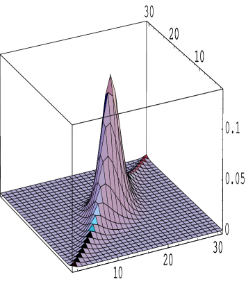
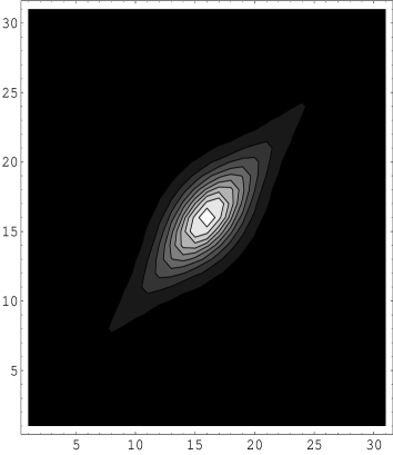
Figure 7: Matrix elements of the exchange interaction $|\langle\Psi_{q(\ell^{\prime})}|1/L_{12}^{2}|\Psi_{q(\ell)}\rangle|$ evaluated between the ${\cal H}_{3/2}$ eigenstates labeled by the integer $\ell,\ell^{\prime}=0,\ldots N+1$ which enumerates the quantized values of $q$ and $q^{\prime}$ from the above, see Sect. 4.5, for $N=30$. The picture to the right shows the contour plot of the 3-dimensional plot.

In contrast to ${\cal H}_{3/2}$, the Hamiltonian ${\cal H}_{1/2}$ is not invariant under cyclic permutations but, still, is symmetric under the interchange of the first and the third quarks, $[{\cal H}_{1/2},{\cal P}_{13}]=0$. This allows to choose its eigenstates to have definite parity with respect to the ${\cal P}_{13}$ permutations

$${\cal H}_{1/2}\Psi^{(\pm)}_{\ell,N}(x_{i})={\cal E}^{(\pm)}_{1/2}(N,\ell)\Psi^{(\pm)}_{\ell,N}(x_{i})\,,\qquad{\cal P}_{13}\Psi^{(\pm)}_{\ell,N}(x_{i})=\pm\Psi^{(\pm)}_{\ell,N}(x_{i})\,.$$ (5.2)

Here, $N$ refers to the total number of derivatives and $\ell$ numerates the energy eigenstates. It is therefore natural to decompose the eigenfunctions $\Psi^{(\pm)}(x_{i})$ over the basis of eigenstates of ${\cal H}_{3/2}$ with definite parity $\Psi_{q,N}^{(\pm)}(x_{i})$ and $q\geq 0$, defined as in (4.20). Using the identity $L_{12}^{-2}+L_{23}^{-2}={\cal P}^{2}L_{13}^{-2}{\cal P}+{\cal P}L_{13}^{-2}{\cal P}^{2}$ and taking into account that the states $\Psi_{q}$ diagonalize the cyclic permutation operator ${\cal P}$ we obtain

$$\langle\Psi_{q^{\prime},N}^{(\pm)}|{V}|\Psi_{q,N}^{(\pm)}\rangle=-2\sqrt{{\cal N}_{q}{\cal N}_{q^{\prime}}}\sum_{m=0}^{N}\frac{f_{m}^{-1}\,u_{m}(q^{\prime})u_{m}(q)}{(m+1)(m+2)}\left[\cos(\phi_{q}-\phi_{q^{\prime}})\pm(-1)^{m}\!\cos(\phi_{q}+\phi_{q^{\prime}})\right],$$ (5.3)

where $u_{n}(q)$ correspond to the expansion coefficients of the ${\cal H}_{3/2}$ eigenfunctions in the $\Psi_{n,N}^{(31)2}$ basis and

$$\langle\Psi_{q^{\prime},N}^{(\pm)}|{V}|\Psi_{q,N}^{(\mp)}\rangle=0\,.$$ (5.4)

The factor

$${\cal N}^{-1}_{q}=\sum_{m=0}^{N}{f_{m}^{-1}u_{m}(q)u_{m}(q)}$$ (5.5)

comes from the normalization condition for the states, which we assume in this section to be $\langle\Psi_{q,N}^{(\pm)}|\Psi_{q,N}^{(\pm)}\rangle=1$.

The explicit calculation gives the spectrum shown in Fig. 8.

Figure 8: The spectrum of eigenvalues for the Hamiltonian ${\cal H}_{12}$. The lines of the largest and the smallest eigenvalues of ${\cal H}_{32}$ are indicated by dots for comparison.

The lines of the largest and the smallest eigenvalues of ${\cal H}_{3/2}$ are indicated by dots for comparison.

As seen from the figure, the spectra of ${\cal H}_{1/2}$ and ${\cal H}_{3/2}$ are very similar in the upper part, for larger eigenvalues, and at the same time the two lowest levels of the ${\cal H}_{1/2}$ Hamiltonian appear to be special and ‘dive’ considerably below the line of lowest eigenvalues of ${\cal H}_{3/2}$, given by Eq. (4.45). Our goal in this section is to explain this structure and to get the quantitative description of the ${\cal H}_{1/2}$ spectrum in the large $N$ limit. Note that at $N\to\infty$ the spectrum of ${\cal H}_{3/2}$ becomes very dense, see Eqs. (4.92), and approaches a continuos spectrum inside the band of the width $\sim 2\ln N$: $4\ln N-6<{\cal E}_{3/2}<6\ln N-6-3\ln 3$. We will demonstrate that exactly the same band of the continuos spectrum is formed for the ${\cal H}_{1/2}$. Inside the band, the distribution of levels is perturbed by corrections at most ${\cal O}(1/N^{2})$ and ${\cal O}(1/\ln^{2}N)$ at the upper and the lower boundary, respectively. In addition, the two lowest eigenstates of ${\cal H}_{1/2}$ (one for each parity) fall below the ‘Fermi surface’ and are separated from the bottom of the band by a finite constant. Existence of such a ‘mass gap’ presents our main result in this section and its formation will be interpreted as due to binding of quarks with opposite chirality by the exchange interaction and formation of scalar diquarks. The eigenfunctions of the ‘bound states’ and the value of the ‘mass gap’ will be estimated.

To visualize both the similarities and the differences between the spectra of ${\cal H}_{3/2}$ and ${\cal H}_{1/2}$ and to trace formation of the ‘mass gap’ for ${\cal H}_{1/2}$, it proves convenient to introduce a somewhat more general Hamiltonian

$${\cal H}(\epsilon)={\cal H}_{3/2}+\epsilon{V}\,,\qquad$$ (5.6)

with $\epsilon$ being a new coupling constant. ${\cal H}(\epsilon=0)$ reproduces ${\cal H}_{3/2}$ whereas ${\cal H}(\epsilon=1)$ coincides with the Hamiltonian ${\cal H}_{1/2}$. Thus, the spectra of ${\cal H}_{3/2}$ and ${\cal H}_{1/2}$ are related to each other through the flow of the energy levels of ${\cal H}(\epsilon)$ from $\epsilon=0$ to $\epsilon=1$, see Fig. 9.

Figure 9: The flow of energy eigenvalues for the Hamiltonian ${\cal H}(\epsilon)$ for $N=29$ and $N=30$, see text. The solid and the dash-dotted curves show the parity-even and parity-odd levels, respectively. The two vertical dashed lines indicate ${\cal H}_{3/2}\equiv{\cal H}(\epsilon=0)$ and ${\cal H}_{1/2}\equiv{\cal H}(\epsilon=1)$, respectively. The horizontal dotted line shows position of the ‘ground state’ given by Eq. (4.45).

Note that for $\epsilon\neq 0$ the Hamiltonian ${\cal H}(\epsilon)$ is neither integrable, nor cyclic symmetric. It is still invariant under conformal transformations and under permutations of the first and the third quarks, $[{\cal H}(\epsilon),{\cal P}_{13}]=0$, but the degeneracy between parity-odd and parity-even eigenstates is lifted and, in fact, the flow of levels with different parity is completely independent from one another.

The spectra in Fig. 9 exhibit the following characteristic features:

1. In the upper part of the spectrum the effect of $\epsilon-$proportional terms on the spectrum of the ‘unperturbed’ Hamiltonian ${\cal H}(\epsilon=0)={\cal H}_{3/2}$ is very mild. While at $\epsilon=0$ the energy levels are double degenerate, their splitting at $\epsilon\neq 0$ remains (exponentially, as we will argue) small for large $N$.

2. For $\epsilon>0$, the two lowest levels are decoupled from the rest of the spectrum and fall off with $\epsilon$ almost linearly. For $\epsilon<0$, the levels with different parity start to cross each other, whereas the flow of the levels with the same parity follows the pattern well known in quantum mechanics as the ‘repulsion of levels’ [36].

This structure suggests that the difference $\epsilon{V}={\cal H}(\epsilon)-{\cal H}(\epsilon=0)$ can be considered as a perturbation for most of the levels, but not for the few lowest ones (for large $N$). To formalize the argument, one has to evaluate the matrix elements in (5.3) and compare them with the energy splittings for the ‘unperturbed’ Hamiltonian. The explicit calculation (see below) gives

$$\langle\Psi_{q^{\prime},N}^{(\pm)}|{V}|\Psi_{q,N}^{(\pm)}\rangle\stackrel{{\scriptstyle q,q^{\prime}\to 0}}{{=}}{\cal O}\left(\frac{1}{\ln N}\right)\,,\qquad\langle\Psi_{q^{\prime},N}^{(\pm)}|{V}|\Psi_{q,N}^{(\pm)}\rangle\stackrel{{\scriptstyle q,q^{\prime}\to 1/\sqrt{27}}}{{=}}{\cal O}\left(\frac{1}{N^{2}}\right)\,.$$ (5.7)

Comparing this result with the level spacings in Eq. (4.92), we conclude that the perturbation theory in ${V}$ is justified for large $N$ (or for small $\epsilon\ll 1$ and arbitrary $N$) for the upper part of the spectrum, while several (of order $\sim\ln N$ as we will find) lowest energy eigenstates are affected strongly and have to be rediagonalized (unless $\epsilon\ll 1/\ln N$). In the sequel, we are going to consider the two different regions separately in more detail.

5.1 Upper part of the spectrum

Eq. (5.3) becomes, for diagonal transitions $q^{\prime}=q$

$$\langle{V}\rangle_{q,N}^{(\pm)}\equiv{\langle\Psi_{q}^{(\pm)}|{V}|\Psi_{q}^{(\pm)}\rangle}=-2{\cal N}_{q}\sum_{m=0}^{N}\frac{f_{m}^{-1}u_{m}^{2}(q)}{(m+1)(m+2)}\left[1\pm(-1)^{m}\cos(2\phi_{q})\right]\,.$$ (5.8)

Each term in the sum is explicitly positive so that the matrix element $\langle{V}\rangle_{q,N}^{(\pm)}$ is always negative meaning that for all levels ${\cal E}_{3/2}-{\cal E}_{1/2}>0$. According to (4.69), the coefficients $u_{m}(q)$ are smooth functions of the scaling variable $x=m/N$, peaked around $x=1/\sqrt{3}$ and rapidly decreasing outside the region $(x-1/\sqrt{3})^{2}\leq\eta^{-1}/3$. Splitting the sum in (5.8) into contributions of even and odd $m$ one finds that the terms proportional to $\cos(2\phi_{q})$ tend to cancel each other and their total contribution is approximately given by the sum of two boundary terms. This contribution is negligible compared to the sum of the phase-independent terms, but at the same time it defines the splitting between energy levels with the different parity

$${\cal E}_{1/2}^{(+)}-{\cal E}_{1/2}^{(-)}\sim\frac{(-1)^{m}f_{m}^{-1}u_{m}^{2}(q)}{(m+1)(m+2)}\bigg{|}_{m_{\rm min}}^{m_{\rm max}}\,.$$ (5.9)

Here $m_{\rm min}/N\ll 1$ and $1-m_{\rm max}/N\ll 1$ define the interval, $m_{\rm min}\leq m\leq m_{\rm max}$, on which the WKB expansion (4.69) is applicable. Applying similar arguments to the sum entering the matrix element

$$0=\langle\Psi_{q}|\Psi_{-q}\rangle\sim\sum_{m=0}^{N}(-1)^{m}f_{m}^{-1}u_{m}^{2}(q)\,,$$ (5.10)

we conclude that the values of $(-1)^{m}f_{m}u_{m}^{2}$ have to coincide at the end points so that

$${\cal E}_{1/2}^{(+)}-{\cal E}_{1/2}^{(-)}\sim\frac{(-1)^{m_{\rm min}}f_{m_{\rm min}}^{-1}u_{m_{\rm min}}^{2}(q)}{(m_{\rm min}+1)(m_{\rm min}+2)}\sim\eta^{-3+\ell}\exp(-\eta)\,.$$ (5.11)

Thus, the splitting between the energy levels of different parity is governed by the tail of the wave function (4.69) and, as a consequence, is exponentially small at large $N$.

Neglecting exponentially small terms and, in particular, the level splitting ${\cal E}_{1/2}^{(+)}-{\cal E}_{1/2}^{(-)}$, we can replace the sum in (5.8) by the integral over the scaling variable $x=m/N$ and substitute the coefficients $u_{m}$ by their WKB expansion (4.66) with the leading term given by (4.69). Substituting this expansion into (5.5) and (5.8) one can calculate the leading and the next-to-leading corrections to the energy (5.8) as

$${\cal E}_{1/2}^{(\pm)}(\ell)-{\cal E}_{3/2}(\ell)\simeq\langle{V}\rangle_{q,N}=-\frac{6}{\eta^{2}}\left[1+\frac{2(2\ell+1)}{\eta}\right]+{\cal O}(1/\eta^{4}),$$ (5.12)

verifying the estimate in (5.7). We remind that $\eta=\sqrt{(N+3)(N+2)}$.

5.2 Lower part of the spectrum

The analysis of the low part of the spectrum is considerably more involved.

We start with calculation of the normalization factor ${\cal N}_{q}$ defined in (5.5). Assuming $\bar{q}\equiv q/\eta^{3}\ll 1$ one can use the WKB approximation (4.76) for $u_{m}(q)$ to get

$${\cal N}_{q}=|\Gamma(1-i\bar{q}N)|^{4}\left(\sum_{n=0}^{[N/2]}1/f_{2n}\right)^{-1}=\frac{2}{3}\eta^{2}\ln^{-1}(\eta\mbox{e}^{\gamma_{E}})\,\left(\frac{\pi\bar{q}N}{\sinh(\pi\bar{q}N)}\right)^{2}\,.$$ (5.13)

This expression defines ${\cal N}_{q}$ to be an exponentially decreasing function of $|\bar{q}|N$. Because of this factor, most of the elements of the $(N+1)\times(N+1)$ matrix ${\langle\Psi_{q}^{(\pm)}|{V}|\Psi_{q}^{(\pm)}\rangle}$ (5.3) are very small, see Fig. 7. It is clear that the off-diagonal matrix elements of this matrix are those responsible for the mixing of different energy levels of the ‘unperturbed’ Hamiltonian and, therefore, strong mixing can only occur if $\bar{q}N,\bar{q}^{\prime}N\sim{\cal O}(1)$. Using the large-$N$ approximate expressions for quantized $q$ (4.83) we may expect that the number of such levels $k_{\rm max}$ is of order $\ln\eta$.

To calculate the matrix elements ${\langle\Psi_{q}^{(\pm)}|{V}|\Psi_{q}^{(\pm)}\rangle}$ given by (5.3) we observe that, unlike in the calculation of ${\cal N}_{q}$, the sum over $m$ is saturated by the contribution of the first few terms, $m\ll N$. Hence $u_{m}(q)$ can be replaced at small $\bar{q}N$ by $u_{2m}=(-1)^{m}+{\cal O}(\bar{q}N)^{2}$ and $u_{2m+1}={\cal O}(\bar{q}N)$, corresponding to the solutions to the recurrence relations (4.72). This gives

$$\langle\Psi_{q^{\prime}}^{(\pm)}|V|\Psi_{q}^{(\pm)}\rangle = -2{\cal N}_{q}\sum_{n={\rm even}}\frac{f_{n}^{-1}}{(n+1)(n+2)}\left[\cos(\phi_{q}-\phi_{q^{\prime}})\pm\cos(\phi_{q}+\phi_{q^{\prime}})\right]$$ (5.14)

$$= -\frac{\pi^{2}}{9}\ln^{-1}(\eta\mbox{e}^{\gamma_{E}})\left[\cos(\phi_{q}-\phi_{q^{\prime}})\pm\cos(\phi_{q}+\phi_{q^{\prime}})\right]\,.$$

The $q-$dependence enters this expression through the phases $\phi_{q}$ and $\phi_{q}^{\prime}$ which take quantized values defined in (4.12). It is easy to see that the possible values of $\cos(\phi_{q}\pm\phi_{q^{\prime}})$ are $1$ and $-1/2$ depending on whether the phases $\phi_{q}$ and $\phi_{q^{\prime}}$ coincide. For the present purpose it turns out to be more convenient to use the basis of eigenstates $\Psi_{q}$ with fixed $q$ rather than fixed parity $\Psi^{(\pm)}_{q}\sim\Psi_{q}\pm\Psi_{-q}$ and write (5.14) in matrix form, introducing an integer $k=[N/2]-\ell$, $k=0,\pm 1,\pm 2,\ldots$ to numerate quantized values of $q$ starting from the ones with the lowest absolute value. We get:

$$\langle\Psi_{q^{\prime}}|\epsilon V|\Psi_{q}\rangle=-g\Lambda_{k^{\prime}k}\,,\qquad\Lambda_{k^{\prime}k}=\left(\begin{array}[]{rrrrr}1&-\frac{1}{2}&-\frac{1}{2}&1&\ldots\\ -\frac{1}{2}&1&-\frac{1}{2}&-\frac{1}{2}&\ldots\\ -\frac{1}{2}&-\frac{1}{2}&1&-\frac{1}{2}&\ldots\\ 1&-\frac{1}{2}&-\frac{1}{2}&1&\ldots\\ \vdots&\vdots&\vdots&\vdots&\ddots\end{array}\right),$$ (5.15)

where, to our accuracy,

$$q=k\frac{\pi\eta^{2}}{6\ln(\eta\mbox{e}^{\gamma_{E}})}\,,$$ (5.16)

and the dependence on $\epsilon$ and $\eta$ is absorbed in the ‘effective coupling’

$$g=\frac{\epsilon\pi^{2}}{9\ln(\eta\mbox{e}^{\gamma_{E}})}.$$ (5.17)

The approximation in (5.15) is justified for $|k|\ll k_{\rm max}={\cal O}(\ln\eta)$.

Imagine, for a moment, that all the participating levels, $|k|<k_{\rm max}$ of the ‘unperturbed’ Hamiltonian ${\cal H}_{3/2}$ were degenerate, i.e. their energy splitting negligible compared to the interaction in (5.15). The true energy eigenstates would coincide then with the eigenstates of the mixing matrix $\Lambda_{kk^{\prime}}$ (of the size $k_{\rm max}$), and the corresponding eigenvalues would define the energies. Remarkably, the spectrum of $\Lambda_{kk^{\prime}}$ is extremely simple. One can easily convince oneself that $\Lambda_{kk^{\prime}}$ has two and only two nonzero eigenvalues which both are equal to $k_{\rm max}$. Remembering that $g\sim 1/\ln\eta$ and $k_{\rm max}\sim\ln\eta$, this implies that two energy levels will get shifted by the finite amount $gk_{\rm max}={\cal O}(\ln^{0}\eta)$ while all the other ones remain exactly degenerate to this accuracy. Since (5.15) was derived up to corrections of order $\sim 1/\ln^{2}\eta$, this implies that the true energy shift for all levels apart from the lowest two ones is at most $\sim 1/\ln^{2}\eta$. This simple heuristic observation explains the pattern observed in Figs. 8, 9.

The real situation is certainly much more complicated. The splitting between lowest energy levels of ${\cal H}_{3/2}$ cannot be neglected, and, in fact, it is precisely this energy splitting which determines the number of lowest states $k_{\rm max}$ that can effectively be considered as degenerate, and the precise value of the ‘mass gap’. For small values of $\bar{q}N$ we can calculate the energies ${\cal E}_{3/2}$ using the asymptotic expression in (4.90) that we rewrite as

$${\cal E}_{3/2}(q)={E}_{0}+\frac{2\zeta(3)\pi^{2}}{9\ln^{2}(\eta\mbox{e}^{\gamma_{E}})}\left(k+\frac{\delta_{N}}{2}\right)^{2}+{\cal O}((\bar{q}N)^{4})\,,\qquad\bar{q}N=k\frac{\pi}{6\ln(\eta\mbox{e}^{\gamma_{E}})},$$ (5.18)

where $k$ is defined as above, ${E}_{0}$ is the ground state energy given by (4.45) and $\delta_{N}=0\,,1$ for even and odd $N$, respectively. Combining together (5.18) and (5.15) we obtain that in the lowest part of the spectrum, corresponding to $\bar{q}N$, $\bar{q}^{\prime}N<1$, the Hamiltonian ${\cal H}(\epsilon)$ can be represented by the following matrix:

$$\langle\Psi_{q^{\prime}}|{\cal H}(\epsilon)-{E}_{0}|\Psi_{q}\rangle = g\left\{\frac{1}{2m}\left[\frac{2\pi}{3}\left(k+\frac{\delta_{N}}{2}\right)\right]^{2}\delta_{k^{\prime}k}-\Lambda_{k^{\prime}k}\right\}\,,$$ (5.19)

$$m = \frac{\pi^{2}}{9\zeta(3)}\epsilon\ln(\eta\mbox{e}^{\gamma_{E}})\,.$$

The corresponding eigenvalue problem is solved in Appendix B. The idea of the solution is to interpret the integer $k$ as a discrete momentum variable. Then, the expression in (5.19) can be considered as an effective Hamiltonian for the low ‘frequency’ $|k|<k_{\rm max}={\cal O}(\ln\eta)$ modes of ${\cal H}(\epsilon)$ and the two terms in the r.h.s. of (5.19) can be identified as the kinetic energy and the periodic potential for a particle on a line. The corresponding wave functions in configuration space correspond to Bloch-Floquet waves and the resulting Schrödinger equation turns out to be a generalization of the famous Kroning-Penney model of a single particle in a periodic $\delta$-function potential. The solution then follows the classical procedure [36].

One has to keep in mind, however, that the effective Hamiltonian in (5.19) presents an approximation to ${\cal H}(\epsilon)$ up to corrections of order ${\cal O}(\bar{q}N)$ and one has to check whether values of $\bar{q}N$ are small on the solutions. It is possible to show that this condition is indeed satisfied for small $\epsilon\ll 1$ (and this is the place where introducing $\epsilon$ as a new parameter starts to play a rôle), see Appendix B. From this analysis we obtain, therefore, a quantitative description of the spectrum of ${\cal H}(\epsilon)$ in the region

$$1/\ln\eta\ll\epsilon\ll 1\,,$$ (5.20)

where the lower bound comes from the condition that the interaction $\epsilon V$ is sufficiently strong to excite many levels.

In agreement with the heuristic argument given above, we find two bound states and the continuum spectrum. The levels in the continuum are $\epsilon$-independent, in the small-$\epsilon$ limit, and are given by

$${\cal E}_{k}={E}_{0}+\frac{\zeta(3)\pi^{2}k^{2}}{8\ln^{2}(\eta\mbox{e}^{\gamma_{E}})},$$ (5.21)

with $1\leq k<\ln\eta$. The two bound states are degenerate up to $1/\eta^{2}-$corrections that we neglected from the beginning and the binding energy (which we identify as a ‘mass gap’) is given by

$$\Delta(\epsilon)={\cal E}_{\rm bound}-{E}_{0}=-\epsilon^{2}\frac{\pi^{4}}{72\zeta(3)}.$$ (5.22)

Comparing this expression with the nonzero eigenvalue of the perturbaton in (5.15), $gk_{\rm max}$, we calculate the number of excited levels of the unperturbed Hamiltonian ${\cal H}_{3/2}$ as $k_{\rm max}=\epsilon\pi^{2}\ln\eta/(8\zeta(3))$, which is in agreement with our expectations.

The low-frequency part of the wave functions of the two bound states coincide for $\ln\eta\to\infty$ with the two lowest energy eigenfunctions of $V$, that are given by the parity even and parity odd combinations of the basis functions (3.38) diagonalizing the Casimir operators $L_{12}^{2}$ and $L_{23}^{2}$:

$$\Psi^{(\pm)}_{\rm bound}(x_{i}) \sim \left[\Psi_{N,n=0}^{(12)3}(x_{i})\pm\Psi_{N,n=0}^{(23)1}(x_{i})\right]+{\cal O}(1/\ln\eta)$$ (5.23)

$$\stackrel{{\scriptstyle\sum x_{i}=1}}{{=}} \left[P^{(3,1)}_{N}(1-2x_{3})\pm P^{(3,1)}_{N}(1-2x_{1})\right]+{\cal O}(1/\ln\eta)\,.$$

This can be seen from the fact that in the limit $\ln\eta\to\infty$ the ‘mass’ $m$ entering (5.19) becomes large and the kinetic term irrelevant. As seen from (5.23), the wave functions have a two-particle structure corresponding to the relative motion of the conformal spin $j=1$ quark with momentum fraction $x_{1}$ (or $x_{3}$) with positive helicity (the first or the third quark, in notations of (2.21)) and an effective particle with momentum fraction $x_{2}+x_{3}$ (or $x_{1}+x_{2}$) and conformal spin $j=2$, which is easily recognized as a scalar diquark. This is in striking contrast to the structure of the lowest energy state for the $\lambda=3/2$ baryons (4.4.2), and in fact the corresponding wave functions are mutually orthogonal in the large$-N$ limit:

$$\langle\Psi^{1/2}_{\rm bound}|\Psi^{3/2}_{0}\rangle\sim 1/\ln\eta.$$ (5.24)

We will further elaborate on the physical interpretation and consequences of this structure in Sect. 6.

Extension of these results to case $\epsilon=1$ is nontrivial since the higher order corrections in $\bar{q}N$ become dominant, and presents a typical strong coupling problem. From Fig. 9 one observes, however, that the quadratic in $\epsilon$ behavior of the bound state energy, (5.22), is replaced by the linear asymptotics starting already from $\epsilon\sim 0.3-0.4$. This suggests to study the energy spectrum of ${\cal H}(\epsilon)$ in the large-$\epsilon$ limit

$$\epsilon\gg 1$$ (5.25)

and try to find an approximate value of the mass gap at $\epsilon=1$ by matching the small-$\epsilon$ and the large-$\epsilon$ expansions. This program is carried out in Sect. 5.3 below.

For completeness, we quote here the results for very small $\epsilon$

$$\epsilon\ll 1/\ln\eta\,,$$ (5.26)

for which case a simple perturbation theory is again valid and the energy shifts are given (up to ${\cal O}(\epsilon^{2})$) by matrix elements of $\epsilon V$ over the eigenstates of the nonperturbed Hamiltonian. For the states with $\phi_{q}=0$ (but $q\neq 0$) we find, for low lying levels

$${\cal E}^{(+)}(\epsilon)-{\cal E}_{3/2}=-2g\,,\qquad{\cal E}^{(-)}(\epsilon)-{\cal E}_{3/2}=0,$$ (5.27)

while for the states with $\phi_{q}=\pm 2\pi/3$ one gets

$${\cal E}^{(+)}(\epsilon)-{\cal E}_{3/2}=-\frac{1}{2}g\,,\qquad{\cal E}^{(-)}(\epsilon)-{\cal E}_{3/2}=-\frac{3}{2}g\,,$$ (5.28)

respectively. Eq. (5.14) is not applicable for calculating the correction to the ground state energy with $q=0$ since this state is not degenerate. A direct calculation of the matrix element $\langle\Psi_{q=0}|V|\Psi_{q=0}\rangle$ based on the exact solutions (4.9) gives

$${\cal E}(\epsilon)-{E}_{0}=-g\,.$$ (5.29)

This relation is exact (to ${\cal O}(\epsilon)$) whereas Eqs. (5.27) and (5.28) are valid up to $O(1/\ln^{3}{h})$ corrections.

5.3 Large$-\epsilon$ expansion

Assuming $\epsilon\gg 1$ is a large parameter, it is natural to invert the logic which we have accepted up to now, and consider ${\cal H}_{3/2}$ as a perturbation of the spectrum of the Hamiltonian $V$ defined in Eq. (5.1).

At the first step, therefore, we have to study the spectrum and the eigenfunctions of $V$ itself. Although the Hamiltonian $V$ is not integrable and cannot be diagonalized exactly, it can be studied in the large $N$ limit using the techniques developed in Refs. [37, 27] for Hamiltonians of similar form. We find that in the leading large$-N$ approximation the eigenstates in the lower part of the spectrum are given by a linear combination of the states diagonalizing the Casimir operators $L_{12}^{2}$ and $L_{23}^{2}$. Their relative coefficient is fixed by the requirement for the eigenstates of $V$ to have definite parity with respect to ${\cal P}_{13}$ permutations

$$\Psi_{V,k}^{(\pm)} = \frac{1}{\sqrt{2}}\left[\Psi_{k}^{(12)3}(x_{1},x_{2},x_{3})\pm\Psi_{k}^{(23)1}(x_{1},x_{2},x_{3})\right]+{\cal O}(\eta^{-2})$$ (5.30)

$$= \frac{1}{\sqrt{2}}\left[\Psi_{k}^{(12)3}(x_{1},x_{2},x_{3})\pm\Psi_{k}^{(12)3}(x_{3},x_{2},x_{1})\right]+{\cal O}(\eta^{-2})\,,$$ (5.31)

where $\Psi_{k}^{(12)3}(x_{i})$ are functions of the conformal basis defined in (3.34), which we assume here to be normalized as $\langle\Psi_{k}^{(12)3}|\Psi_{n}^{(12)3}\rangle=\delta_{kn}$. The corresponding eigenvalues, ${\cal E}^{(\pm)}_{V}=\langle\Psi_{V,k}^{(\pm)}|\epsilon V|\Psi_{V,k}^{(\pm)}\rangle$ can be evaluated using (3.37) and (A.4) as

$$\epsilon^{-1}\,{\cal E}_{V}^{(\pm)}(k)=-\frac{1}{(k+1)(k+2)}-\sum_{m=0}^{N}\frac{\Omega_{km}^{2}\Omega_{mk}}{(m+1)(m+2)}\mp\frac{\Omega_{kk}}{(k+1)(k+2)}+{\cal O}(\eta^{-4})\,.$$ (5.32)

Taking into account Eqs. (A.15) and (A.19) we find

$${\cal E}_{V}^{(\pm)}(k)=-\frac{\epsilon}{(k+1)(k+2)}-\epsilon\eta^{-2}\left[1\pm(-1)^{N+k}\right](2k+3)+{\cal O}(\eta^{-4})\,.$$ (5.33)

Here, the integer $k=0\,,1\,,2,\ldots$ enumerates the levels of $V$ with definite parity starting from the lowest one. We observe that for given conformal spin $N$ the nonleading ${\cal O}(\eta^{-2})$ corrections vanish for each second level leading to ${\cal E}_{V}^{(\pm)}(k)=-\epsilon/[(k+1)(k+2)]$ provided that $k+N={\rm even~{}(odd)}$ for levels with positive (negative) parity. It can be shown that this result is exact to all orders in $1/\eta$.

The nonleading ${\cal O}(\eta^{-2})$ corrections remove degeneracy of the levels

$${\cal E}_{V}^{(+)}(k)-{\cal E}_{V}^{(-)}(k)=-2\epsilon\,(2k+3)(-1)^{N+k}\eta^{-2}+{\cal O}(\eta^{-4})\,.$$ (5.34)

Thus, in the lowest part of the spectrum, $k\ll N$, the eigenvalues of the Hamiltonian $V$ belong to the two trajectories,

$${\cal E}_{V,{\rm up}}(k) = -\frac{\epsilon}{(k+1)(k+2)}\,,\qquad$$

$${\cal E}_{V,{\rm down}}(k) = {\cal E}_{V,{\rm up}}(k)-2\epsilon(2k+3)\eta^{-2}+{\cal O}(\eta^{-4})$$ (5.35)

parameterized by a nonnegative integer $k$. Parity of the eigenstates alternates along each trajectory.

At the second step, we evaluate the matrix elements of ${\cal H}_{3/2}$ over the eigenstates of $V$ defined in Eq. (5.31). Using (A.21) and (5.31) one can write

$$\frac{1}{2}\left[\langle\Psi_{V,k}^{(+)}|{\cal H}_{3/2}|\Psi_{V,k}^{(+)}\rangle+\langle\Psi_{V,k}^{(-)}|{\cal H}_{3/2}|\Psi_{V,k}^{(-)}\rangle\right] = \varepsilon(k)+2\sum_{m=0}^{N}(-1)^{m+k}\Omega_{km}\varepsilon(m)\Omega_{mk}\,,$$ (5.36)

$$\frac{1}{2}\left[\langle\Psi_{V,k}^{(+)}|{\cal H}_{3/2}|\Psi_{V,k}^{(+)}\rangle-\langle\Psi_{V,k}^{(-)}|{\cal H}_{3/2}|\Psi_{V,k}^{(-)}\rangle\right] = 2\varepsilon(k)\Omega_{kk}+\sum_{m=0}^{N}\Omega_{km}\varepsilon(m)\Omega_{mk},$$ (5.37)

where $\varepsilon(m)=2[\psi(m+2)-\psi(2)]]$ is the two-particle energy. The sums over $m$ are dominated by contributions of $x\equiv m/N={\cal O}(1)$. Therefore, replacing $\varepsilon(m)=2\ln(Nx)-2\psi(2)$ and using properties of the Racah $6j-$symbols, (A.4), (A.15) and (A.19), we get for the parity-averaged spectrum of ${\cal H}(\epsilon)$

$${\cal E}^{(\pm)}(\epsilon) = {\cal E}_{V}^{(\pm)}(k)+\langle\Psi_{V,k}^{(\pm)}|{\cal H}_{3/2}|\Psi_{V,k}^{(\pm)}\rangle+{\cal O}(1/\epsilon),$$ (5.38)

$$\langle\Psi_{V,k}^{(\pm)}|{\cal H}_{3/2}|\Psi_{V,k}^{(\pm)}\rangle = 4\ln\eta-6\psi(2)+6\psi(k+2)-4\psi(2k+4)+\!\frac{2}{k+2}+\!\frac{2}{2k+3}+\!{\cal O}(\eta^{-1}),$$

while the energy splitting between the eigenstates with opposite parity equals

$${\cal E}^{(+)}(\epsilon)-{\cal E}^{(-)}(\epsilon)={\cal E}^{(+)}_{V}(\epsilon)-{\cal E}^{(-)}_{V}(\epsilon)~{}+$$ (5.39)

$$+ 4\left[\ln\eta+2\psi(k+2)-3\psi(2)\right]\eta^{-2}(-1)^{N+k}(2k+3)(k+1)(k+2)\,.$$

For large $\eta$ the correction terms in both cases are dominated by the first term $\sim\ln\eta$ which can be related to the ‘ground state’ energy ${E}_{0}$ of the Hamiltonian ${\cal H}_{3/2}$ defined in (4.45). It provides an overall shift of all levels and can be absorbed into the definition of the nonperturbed Hamiltonian $V$. Then, comparing the matrix elements (5.38) with the level spacing in the $V$-spectrum in (5.33), we conclude that the large$-\epsilon$ expansion is well-defined for $\epsilon\gg 1$.

In particular, for the lowest level $k=0$ we obtain:

$$\Delta(\epsilon)={\cal E}(\epsilon)-{E}_{0}=-\frac{1}{2}\epsilon+\frac{1}{3}+{\cal O}(\epsilon^{-1}).$$ (5.40)

One should stress that all the above expressions are only valid for the lowest levels $k\ll N$ in the spectrum.

It is instructive to examine the flow of the energy levels defined by the perturbative expressions (5.33) and (5.38). Varying $\epsilon$ from $\epsilon=\infty$ towards $\epsilon=1$ we find that the energy levels are changing linearly in $\epsilon$, with the slope depending on integer $k$ and on the parity of the level. The perturbative correction generates the $\epsilon-$independent shift of the trajectories whose amount again depends on the parity and $k$. The ‘critical’ values of $\epsilon$ at which the linear trajectories cross the ground state energy ${E}_{0}={\cal E}_{3/2}(q=0)$ set up the low boundary for $\epsilon$ such that the $1/\epsilon-$expansion is applicable. Using (5.33) and (5.38) we find the corresponding intersection points as

$$\epsilon_{\rm crit}(k=0)=0.66\,,\qquad\epsilon_{\rm crit}(k=1)=5.60\,,\qquad\epsilon_{\rm crit}(k=2)=16.97\,.\qquad$$ (5.41)

These values are in a good agreement with the numerical solutions shown in Fig. 9.

Finally, notice that the $1/\epsilon-$expansion can also be applied to describe the flow of energy levels for $\epsilon<0$ but its range of the applicability is in this case only $-\infty\ll\epsilon\ll-\ln\eta$. The main difference between positive and negative $\epsilon$ is that in the latter case the lowest energy levels of the Hamiltonian ${\cal H}(\epsilon)$ are rapidly approaching each other for $-\ln\eta\ll\epsilon<0$. As a consequence, the naive $1/\epsilon-$expansion becomes divergent due to small denominators and should be replaced by the so-called ‘degenerate perturbative expansion’.

5.4 Estimate of the mass gap

Having derived the asymptotic expressions for the mass gap $\Delta(\epsilon)$ in the two limits $\epsilon\ll 1$ and $\epsilon\gg 1$, Eqs. (5.22) and (5.40), respectively, we can make an estimate for $\epsilon\sim 1$ by matching the two expansions. To this end, we design an interpolating Padé formula:

$$\Delta(\epsilon)=-\frac{\epsilon^{2}(\kappa+\alpha\epsilon)}{1+2(\kappa+2\alpha/3)\epsilon+2\alpha\epsilon^{2}},$$ (5.42)

with $\kappa=\pi^{4}/(72\zeta(3))=1.12549$, which reproduces (5.22) and (5.40) in the appropriate limits and contains one free parameter $\alpha$ that has to be positive in order to avoid spurious singularities. Allowing $\alpha$ to vary within the extreme limits $0<\alpha<\infty$ we get

$$\Delta_{1/2}\equiv\Delta(\epsilon=1)=-(0.30000-0.34620)\,,$$ (5.43)

which compares very well with the result of the direct numerical calculation of the parity average energy of the lowest eigenstates at $N=300$:

$$\frac{1}{2}\Big{[}{\cal E}_{1/2}^{(+)}+{\cal E}_{1/2}^{(-)}\Big{]}-{E}_{0}=-0.32097\,.$$ (5.44)

The results of the numerical calculation of the lowest few eigenvalues of ${\cal H}_{1/2}$ are shown in Fig. 10.

Figure 10: The difference ${\cal E}_{1/2}-{E}_{0}$ for the first few energy levels.

It is seen clearly that the distance between the two lowest eigenvalues and the ‘vacuum energy’ ${E}_{0}$ approaches a constant $\sim 0.3$, while for higher levels this distance decreases as $1/\ln^{2}N$. Notice, however, that the distance to ${E}_{0}$ and the level splittings for higher levels are still quite large for $\ln N\sim 5$ ($N\sim 10^{2}$). The reason for this is that the expansion parameter for the upper part of the spectrum proves to be $1/\ln N$ (rather than $1/N$) and the asymptotic large$-N$ limit is, therefore, approached very slowly.

6 Distribution amplitudes $\phi^{3/2}_{\Delta}$, $\phi^{1/2}_{\Delta}$, $\phi^{1/2}_{N}$: Summary of results

In this section we give a short summary of the results of phenomenological relevance for the physical baryon distribution amplitudes defined in Sect. 2.1 and discuss an overall physical picture that emerges.

The Brodsky-Lepage evolution equation for the helicity-$3/2$ distribution amplitude $\phi^{3/2}_{\Delta}$ is exactly integrable and is considered in much detail in Sect. 4. The physical interpretation of integrability is that we are able to identify a new ‘hidden’ quantum number which distinguishes components in the $\Delta$-resonance with different scale dependence. The anomalous dimensions and the eigenfunctions can be calculated in this case exactly using a simple three-term recurrence relation given in Eq. (4.3). The coefficients $u_{n}$ define the expansion coefficients (3.32) for the eigenfunctions of the evolution equation over the complete set of mutually orthogonal conformal polynomials (3.42) and the corresponding anomalous dimensions are given in terms of the same coefficients by Eqs. (4.43) and (2.33). Alternatively, we have derived a systematic WKB-type expansion for large values of $N$ which provides one with a systematic expansion of the eigenvalues, [see Eqs.  (4.71), (4.81), (4.83), (4.85)] and the eigenfunctions [see Eqs. (4.101), (4.106), (4.102)], in powers of $1/N$.

The case of $\phi^{3/2}_{\Delta}$ is still specific as compared to the general treatment in Sect. 4 in that neglecting tiny $SU(2)$-flavor violation effects due to quark masses $\phi^{3/2}_{\Delta}$ is totally symmetric in all three arguments. As a consequence, only one third of the existing multiplicatively renormalisable operators have nonvanishing matrix elements, namely, those corresponding to the unity eigenvalue $\theta=1$ of the cyclic permutation operator. Note that the value of $\theta$ alternates along the trajectories shown in Fig. 2 so that each third of the eigenvalues gives a relevant contribution.

Recall that each eigenvalue in Fig. 2 (except for the lowest one for each $N$) is double degenerate. The two degenerate eigenstates can be chosen either as eigenstates of the $Q$-operator with opposite sign eigenvalues $q$ and $-q$, or as states with definite parity, defined in Eq. (4.20). The latter choice is more convenient since the parity eigenfunctions are real and contributions to $\phi^{3/2}_{\Delta}$ of the operators with negative parity vanish identically. One is left with the sum over positive parity eigenstates with real coefficients.

The most interesting result concerns the structure of the eigenstates with the lowest eigenvalue (anomalous dimension) for each $N$ which present, therefore, the leading contributions to the distribution amplitude in the formal $\mu^{2}\to\infty$ limit:

$$x_{1}x_{2}x_{3}\Psi^{3/2}_{N}(x_{1},x_{2},x_{3})=$$

$$= x_{1}(1-x_{1})\,C_{N+1}^{3/2}(1-2x_{1})+x_{2}(1-x_{2})\,C_{N+1}^{3/2}(1-2x_{2})+x_{3}(1-x_{3})\,C_{N+1}^{3/2}(1-2x_{3})\,,$$

see Fig. 11.

   

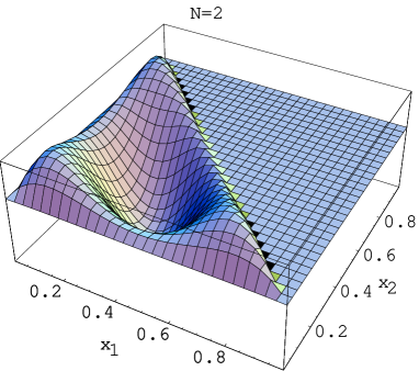
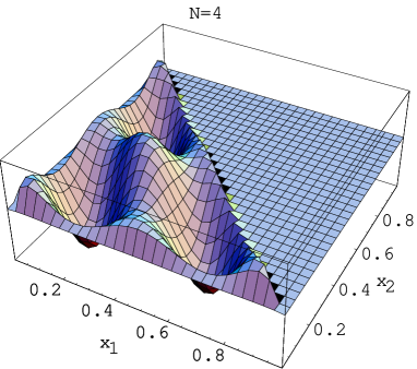
Figure 11: Contributions to the $\lambda=3/2$ distribution amplitude $\phi_{\Delta}^{3/2}(x_{i})$ with lowest anomalous dimensions for $N=2$ and $N=4$. The normalization is arbitrary.

The corresponding eigenvalues are known exactly and are given in Eq. (4.45).

The physical interpretation of such ‘ground states’ is most transparent in coordinate space. Neglecting the operators with total derivatives, which amounts to going over from (6) to the distribution function $\widetilde{\Psi}$ of one variable in Eq. (4.47), one can represent the three-quark ‘ground state’ in a concise form as the nonlocal light-cone operator [38]

$$B_{3/2}^{(q=0)}(z_{1},z_{2},z_{3})=\frac{1}{2}\sum_{\alpha,\beta=1,2,3\atop\alpha\neq\beta}\varepsilon^{ijk}\int_{0}^{1}\!dv\,\!\not\!nq_{i}^{\uparrow}(z_{\alpha}n)\!\not\!nq_{j}^{\uparrow}([vz_{\alpha}+(1-v)z_{\beta}]n)\!\not\!nq_{k}^{\uparrow}(z_{\beta}n)$$ (6.2)

The Tailor expansion of the forward matrix elements of (6.2) at short distances, $z_{12},z_{32}\to 0$, generates the series of local multiplicatively renormalizable three-quark local operators with the lowest anomalous dimension for each even $N$

$$B_{3/2}^{(q=0)}(z_{1},z_{2},z_{3})=\sum_{N={\rm even}}\frac{z_{12}^{N}+z_{23}^{N}+z_{31}^{N}}{(N+1)!}\ \Psi_{N,q=0}^{3/2}(\partial_{1},\partial_{2},\partial_{3})\ B(z_{1},z_{2},z_{3})\bigg{|}_{z_{\alpha}=0\,,\atop\partial_{1}+\partial_{2}+\partial_{3}=0}$$ (6.3)

Note integration in (6.2) with unit weight over the position of the quark in the middle that goes in between the light-cone positions of the other two quarks, up to permutations. If renormalization of the operator is interpreted as interaction, integration with the unit weight can in turn be interpreted as the statement that the quark in the middle is effectively ‘free’: In the ‘ground state’ with the lowest ‘energy’, the interaction of the quark in the middle with its right and left neighbours exactly compensate each other.

The evolution equations for helicity-1/2 distribution amplitudes $\phi^{1/2}_{\Delta}$ and $\phi^{1/2}_{N}$ differ from the evolution equation for $\phi^{3/2}_{\Delta}$ by the additional contribution of gluon exchange between the quarks with opposite helicity, see Eq. (2.26) and Fig. 1. The added terms destroy exact integrability, but, as we found, can be considered as a small perturbation for the upper part of the spectrum. As a consequence, there is a direct correspondence between eigenoperators and anomalous dimensions for helicity-3/2 and helicity-1/2 distributions and the corrections can be calculated to $1/N^{3}$ accuracy using the standard quantum-mechanical perturbation theory, see Eq. (5.12). The splitting between the eigenstates with opposite parity proves to be exponentially small at large $N$, see Eq. (5.11).

For low-lying levels the situation turns out to be dramatically different. We find that the two lowest eigenvalues (anomalous dimensions) decouple from the rest of the spectrum and in the limit $\ln N\to\infty$ are separated from the other eigenvalues by a finite constant $\Delta\sim-0.3$ (5.43) that we call the ‘mass gap’. The corresponding contributions to the distribution amplitudes are given by

$$x_{1}x_{2}x_{3}\Psi^{1/2}_{N\to\infty}(x_{1},x_{2},x_{3})=x_{1}x_{2}x_{3}\left[P^{(3,1)}_{N}(2x_{3}-1)\pm P^{(3,1)}_{N}(2x_{1}-1)\right]$$ (6.4)

where $P^{(3,1)}_{N}$ are Jacobi polynomials, and correspond, in the same sense as above, to the contribution of the nonlocal light-cone operator

$$B(z_{1},z_{2},z_{3})=$$ (6.5)

$$= \varepsilon^{ijk}\left[(\!\not\!nq_{i}^{\uparrow}\!\not\!nq_{j}^{\downarrow})(z_{1}n)\!\not\!nq_{k}^{\uparrow}(z_{3}n)\delta(z_{2}-z_{1})\pm\!\not\!nq_{i}^{\uparrow}(z_{1}n)(\!\not\!nq_{j}^{\downarrow})\!\not\!nq_{k}^{\uparrow})(z_{3}n)\delta(z_{2}-z_{3})\right]$$

Formation of the mass gap in the spectrum of anomalous dimensions is, therefore, naturally interpreted as due to binding of the quarks with opposite helicity and forming scalar diquarks.

Note that while the expression for the eigenfunction in (6) is exact, the result in (6.4) is only valid in the asymptotic $\ln N\to\infty$ limit. In the coordinate space picture, the restriction to large $N$ is translated to the condition that the light-cone separation between the same helicity quarks is very large to allow for the formation of a diquark. In momentum space, the result means that at sufficiently large scales $Q^{2}$ the quark carrying a very large momentum fraction is more often with the same helicity as of the parent baryon. This observation seems to be in qualitative agreement with phenomenological models of baryon distribution amplitudes derived from QCD sum rules [19, 20].

     

Figure 12: The ‘ground state’ eigenfunctions $\widetilde{\Psi}(x)$ for the Hamiltonians ${\cal H}_{1/2}$ (solid), ${\cal H}_{3/2}$ (long dashes) and $V$ (short dashes) for $N=19$. The normalization is to unit integral $\int\!dx\,\widetilde{\Psi}(x)=1$ and to the unit first moment $\int\!dx\,x\,\widetilde{\Psi}(x)=1$ for the symmetric and the antisymmetric wave functions, respectively.

One has to keep in mind, however, that the diquark picture of the states with the lowest anomalous dimensions only becomes quantitative for very large $N$. To illustrate this point, we plot in Fig. 12 the exact eigenfunctions $\widetilde{\Psi}$ for ${\cal H}_{1/2}$ at $N=19$ (with positive and negative parity) corresponding to the lowest anomalous dimensions (solid curves), and compare them both with the lowest-level eigenfunctions for ${\cal H}_{3/2}$ (dashes) and with the ‘diquark’ eigenfunction corresponding to Eq. (6.4) (dots). It is seen that the eigenfunctions of ${\cal H}_{1/2}$ for this value of $N$ are still very close to ${\cal H}_{3/2}$ and only start to develop small ‘horns’ close to the end points, characteristic for the diquark picture. As mentioned above, the true large-$N$ limit is approached very slowly since parameter of the expansion is in this case $1/\ln N$ rather than $1/N$.

7 Conclusions

To summarize, in this paper we have developed a new theoretical framework for the description of baryon distribution amplitudes in QCD, based on integrability of the helicity–3/2 Brodsky-Lepage evolution equation. The mathematical structure of the evolution equations reflects a clear physical structure of the distribution amplitudes that we tried to emphasize. A lot of analytic results is obtained, in different limits.

The formalism proposed in this paper is rather general and can be applied, as indicated in [15], to the studies of quark-antiquark-gluon and, possibly, three-gluon distributions.

Three general questions related to the theory of three-particle distributions are not covered in this work and deserve further attention. First, as we have indicated, analytic continuation of the spectrum of anomalous dimensions of three-particle operators to the complex angular momentum plane is intrinsically ambiguous. One has to study whether this mathematical ambiguity is resolved by imposing certain physical conditions on the amplitudes. Second, the solution of the evolution equations for three-particle distributions depends on the nonpertrubative initial conditions. Depending on the choice of the three-particle distribution amplitudes at low scales, there is a possibility that at large evolution times the solutions to the evolution equation become independent on the initial conditions and are governed entirely by perturbative evolution. Such perturbatively driven distribution amplitudes would generalize the GRV partonic distributions [39] which prove to be successful in the phenomenology of hard inclusive processes. Finally, the integrability of the evolution equations reveals an additional hidden symmetry of QCD and its close relation to exactly solvable statistical models. Remarkably enough the same symmetry has been observed in the studies of the Regge asymptotics of three-particles distributions. These properties are not seen at the level of the QCD Lagrangian and their origin needs to be understood better.

Acknowledgments

V.B., S.D. and A.M. would like to thank L.N. Lipatov, and G.K. is grateful to A.B. Kaidalov for useful discussions. Our special thanks are due to A.V. Belitsky for the critical reading of the manuscript. This work was supported in part by NORDITA through the Baltic Fellowship program funded by the Nordic Council of Ministers, by Russian Fond of Basic Research, Grant 97–01–01152 (S.D. and A.M.) and by the EU networks ‘Training and Mobility of Researchers’, contracts EBR FMRX–CT96–008 (V.B.) and FMRX–CT98–0194 (G.K.).

Appendix A Appendix: Racah $6j$-symbols of the $SL(2)$ group

The functions $\Psi^{(12)3}_{N,n}(x_{i})$ introduced in Sect. 3.4 have a simple group theory interpretation. They define the addition rules for the sum of three conformal spins $j=1$ each corresponding to the $SL(2)$ generators $L_{\alpha,k}$ ($k=1\,,2\,,3$) acting on the light-cone coordinates of three quarks and the superscript $(12)3$ indicates the order in which the tensor product of three $SL(2)$ representations has been decomposed into the irreducible components for which $\Psi^{(12)3}_{N,n}(x_{i})$ is the highest weight. According to (3.34) and (3.36), $\Psi^{(12)3}_{N,n}(x_{i})$ describes the irreducible component for which the total conformal spin is $h=N+3$ and the conformal spin in the channel $(12)$ is equal to $j_{12}=n+2$. Changing the order in which the spins are added one obtains an equivalent basis of functions $\Psi^{1(23)}_{n}(x_{i})$ that are linear related to $\Psi^{(12)3}_{n}(x_{i})$ through the Racah decomposition (3.37). The coefficients $\Omega_{kn}$ thus define the $6j-$symbols for the discrete positive series of the $SL(2)$ group. It is easy to see that the corresponding basis functions are transformed into each other by cyclic permutations

$$\Psi^{1(23)}_{N,n}(x_{1},x_{2},x_{3})=\Psi^{(12)3}_{N,n}(x_{2},x_{3},x_{1})$$ (A.1)

and, therefore, the $(N+1)\times(N+1)$ matrix $\Omega$ represents the operator of cyclic permutations ${\cal P}$ (4.10) in the conformal basis

$$\langle\Psi_{m}^{(12)3}|\Psi_{n}^{1(23)}\rangle=\langle\Psi_{m}^{(12)3}|{\cal P}|\Psi_{n}^{(12)3}\rangle=\Omega_{nm}\frac{60f_{m}}{(2N+5)},$$ (A.2)

where we used the expression for the norm of the basis vectors (3.39). Since $\Psi_{n}^{(12)3}$ is a real function of $x_{i}$, the calculation of the scalar product leads to real matrix elements

$$\Omega_{nm}^{*}=\Omega_{nm}\,,\qquad\sum_{n=0}^{N}f_{n}\Omega_{ln}\Omega_{mn}=f_{m}\delta_{ml}\,,$$ (A.3)

where the second relation is the unitarity condition. Since ${\cal P}^{3}=1$ and ${\cal P}^{2}={\cal P}_{12}{\cal P}{\cal P}_{12}={\cal P}^{-1}$, the matrix $\Omega$ has to satisfy the following conditions:

$$\Omega^{3}_{nm}=\delta_{nm}\,,\qquad\Omega^{2}_{nm}=(-1)^{n+m}\Omega_{nm}=\Omega^{-1}_{nm}\,,$$ (A.4)

where in the last relation we used the identity

$${\cal P}_{12}\Psi^{1(23)}_{N,n}(x_{1},x_{2},x_{3})=\Psi^{1(23)}_{N,n}(x_{2},x_{1},x_{3})=(-1)^{n}\Psi^{1(23)}_{N,n}(x_{1},x_{2},x_{3})\,.$$ (A.5)

Explicit expressions for the matrix elements $\Omega_{kn}$ can be obtained in terms of the ${}_{4}F_{3}-$hypergeometric series of unit argument [40]. To show this, consider the defining relation (3.37) and choose $x_{1}=-x_{2}=x$ and $x_{3}=1$ so that $x_{1}+x_{2}+x_{3}=1$ and $x_{1}+x_{2}=0$ and $\Psi_{n}^{(12)3}(x_{i})$ reduces to $x^{n}$ up to a numerical factor. Rewriting the Gegenbauer and Jacobi polynomials in terms of hypergeometric functions, one brings Eq. (3.37) to the form

$${}_{2}F_{1}{\left({{-m,-m-1\atop 2}\bigg{|}x}\right)}\,{}_{2}F_{1}{\left({{-N+m,N+m+5\atop 2m+4}\bigg{|}x}\right)}\rho_{m}=\sum_{n=0}^{N}\Omega_{mn}x^{n}\sigma_{n}$$ (A.6)

where

$$\sigma_{n} = (-1)^{N-n}\frac{(N+n+4)!}{(n!)^{2}(N-n)!}\frac{1}{(2n+2)(2n+3)},$$

$$\rho_{m} = \frac{1}{2}(-1)^{m}(m+1)(m+2)\frac{(N+m+4)!}{(N-m)!(2m+3)!}.$$ (A.7)

The two hypergeometric functions entering (A.6) are polynomials in $x$ of degree $m$ and $N-m$, respectively. Their product defines the generating function for the matrix elements $\Omega_{mn}$. Expanding the l.h.s. of A.6 in powers of $x$, one can write the coefficient of $x^{n}$ as the ${}_{4}F_{3}-$function of unit argument and identify it with $\Omega_{mn}$. Explicit expressions for arbitrary $N$ and $n$ are rather cumbersome, see, e.g., [41].

We are able, however, to find a simple approximate expressions for $\Omega_{mn}$ which are valid in the WKB limit of large spins $N$. To this end, notice that the matrix elements $\Omega_{nm}$ satisfy second-order finite difference equations. One finds them by applying the operator $L_{23}^{2}$ to the both sides of (3.37) and taking into account (3.40)

$$2(m+2)(m+1)\Omega_{mn}=\frac{f_{n+1}}{n+2}\Omega_{m,n+1}+\frac{(2n+3)f_{n}}{(n+1)(n+2)}\Omega_{m,n}+\frac{f_{n-1}}{n+1}\Omega_{m,n-1}\,,$$ (A.8)

where $m,n=0,\ldots,N$ and $\Omega_{m,-1}=0$. Let

$$\Omega_{mn}=(-1)^{n}\frac{\omega_{m}(n)}{f_{n}}$$ (A.9)

so that Eqs. (A.8) and (A.3) are replaced by

$$2(m+2)(m+1)\omega_{m}(n)=-\frac{f_{n}}{n+2}(\omega_{m}(n+1)-\omega_{m}(n))+\frac{f_{n}}{n+1}(\omega_{m}(n)-\omega_{m}(n-1)),$$

$$\sum_{n=0}^{N}\frac{1}{f_{n}}\omega_{m}(n)\omega_{l}(n)=f_{m}\delta_{ml},$$ (A.10)

$$\omega_{m}(n)=\omega_{n}(m),$$

defining the system of orthogonal polynomials $\omega_{m}(n)$ in the discrete variable $n$ with $m=0,\ldots,N$. The initial condition for the recurrence relations in (A.10) can be found from the relation $\Phi^{1(23)}_{k}(z_{i})=\sum_{n=0}^{N}\Omega_{kn}\Phi^{(12)3}_{n}(z_{i})$ in the limit $z_{1}-z_{2}\to 0$ using (3.55) and (3.56) as

$$\omega_{n}(0)=\frac{2(-1)^{N}}{(N+2)(N+3)}f_{n}(2n+3)\,.$$ (A.11)

There are two limiting cases when the recursion relations for $\omega_{m}(n)$ can be solved analytically. In the first case, in the limit

$$x=\frac{n}{N}=\mbox{fixed}\,,\quad m=\mbox{fixed}\,,\quad N\to\infty$$ (A.12)

the recurrence relation in (A.10) is reduced to the differential equation on the function $\omega_{m}(n)\to\omega_{m}(x)$

$$\omega^{\prime\prime}_{m}(x)-\frac{1}{x}\omega_{m}^{\prime}(x)+\frac{4(m+2)(m+1)}{1-x^{2}}\omega_{m}(x)=0\,.$$ (A.13)

Picking up the polynomial solution we obtain

$$\omega_{m}(x)=N^{2}x^{2}(1-x^{2})C_{m}^{3/2}(1-2x^{2})\,.$$ (A.14)

The normalization is fixed by the second relation in (A.10) where one replaces $\sum_{n}\to N\int_{0}^{1}dx$. Finally, substituting (A.14) into (A.9) we get

$$\Omega_{mn}=\frac{4(-1)^{n}}{N}xC_{m}^{3/2}(1-2x^{2})\,,\qquad n=xN\,,$$ (A.15)

which is valid to $O(1/N)$ accuracy in the limit specified in (A.12).

In the second case, in the limit

$$n\,,m=\mbox{fixed}\,,\quad N\to\infty$$ (A.16)

the recurrence relation in (A.10) is reduced to the condition

$$\frac{1}{n+2}(\omega_{m}(n+1)-\omega_{m}(n))=\frac{1}{n+1}(\omega_{m}(n)-\omega_{m}(n-1))\,.$$ (A.17)

Its solution satysfying (A.11) is given by

$$\omega_{m}(n)=\frac{1}{2}(-1)^{N}(n+1)(n+2)(m+1)(m+2)\times\left[1+{\cal O}(1/N^{2})\right]$$ (A.18)

leading to

$$\Omega_{mn}=N^{-2}(-1)^{N+n}(2n+3)(m+1)(m+2)\times\left[1+{\cal O}(1/N^{2})\right]\,.$$ (A.19)

Having defined the matrix $\Omega_{nm}$ it becomes straightforward to calculate matrix elements of the Hamiltonians ${\cal H}_{3/2}$ and ${\cal H}_{1/2}$ in the conformal basis. To this end we write

$${\cal H}_{3/2}={\cal H}_{12}+{\cal P}{\cal H}_{12}{\cal P}^{-1}+{\cal P}^{2}{\cal H}_{12}{\cal P}^{-2}$$ (A.20)

and similar for ${\cal H}_{1/2}$. Then, applying this identity to a basis function $\Psi^{(12)3}_{n}(x_{i})$ and using the properties (A.4) of the $\Omega-$matrix we find that ${\cal H}_{3/2}$ can be represented in the conformal basis by the $(N+1)\times(N+1)$ matrix $[{\cal H}_{3/2}]_{nk}$

$${\cal H}_{3/2}\Psi^{(12)3}_{n}=\sum_{k=0}^{N}[{\cal H}_{3/2}]_{nk}\Psi^{(12)3}_{k},$$ (A.21)

$$[{\cal H}_{3/2}]_{nk}=\varepsilon(n)\delta_{nk}+[(-1)^{n}+(-1)^{k}]\sum_{m=0}^{N}(-1)^{m}\Omega_{nm}\varepsilon(m)\Omega_{mk},$$

where $\varepsilon(n)$ is the energy of the two-particle Hamiltonian defined in (4.40). It is easy to see that this derivation relies on the two-particle structure of the Hamiltonian only and is not sensitive to integrability properties. In particular, the similar representation holds for the Hamiltonian ${\cal H}_{1/2}$, with $\varepsilon(m)$ in the sum over $m$ shifted by the exchange interaction term $1/[(m+2)(m+1)]$.

Appendix B Appendix: The low-energy effective Hamiltonian for ${\cal H}(\epsilon)$

The eigenproblem for the matrix (5.19) takes a well known form once we interpret the integer $k$ as a discrete momentum variable. Denoting the corresponding eigenvector as $\vec{c}=\{c_{k}\}$ we construct the wave function in the configuration $x-$space as

$$\chi(x)=\sum_{k=-k_{\rm max}}^{k_{\rm max}}c_{k}\,\mbox{e}^{\frac{2i\pi}{3}x(k+\delta_{N}/2)}\,.$$ (B.1)

The restriction to $|k|\leq k_{\rm max}$ serves to remind that (5.19) presents an approximation to the Hamiltonian ${\cal H}(\epsilon)$ which is only valid for $|k|\ll\ln\eta$. It is natural to expect that the lowest energy levels of the matrix (5.19) are not sensitive to the UV cut-off $k_{\rm max}$, or, equivalently, the corresponding eigenstates $\chi(x)$ are smooth functions of $x$ at short distances $\Delta x\sim 1/\ln\eta$. To the extent that this ‘decoupling’ property holds true, which we are going to verify a posteriori, the low-lying levels of the Hamiltonian ${\cal H}(\epsilon)$ coincide with the lowest eigenstates of (5.19) so that the latter can be considered as the effective low-energy Hamiltonian for the former. Having this in mind, we temporally send the UV cutoff $k_{\rm max}$ to infinity and assume the matrix (5.19) to be of infinite size.

Using the transformation (B.1) one can map the eigenproblem for the matrix (5.19) into a one-dimensional Schrödinger equation for the wave function $\chi(x)$. It follows from (B.1) that $\chi(x)$ is a (anti)periodic function of $x$ with the period $3$ for even (odd) values of $N$, respectively:

$$\chi(x+1)=(-1)^{N}\chi(x)\,.$$ (B.2)

The two cases should, therefore, be treated separately. Let us first consider the case of even $N$ and split the wave function into the sum of three terms

$$\chi(x) = \chi_{+}(x)+\chi_{-}(x)+\chi_{0}(x),$$ (B.3)

$$\chi_{\alpha} = \sum_{k=-\infty}^{\infty}c_{3k+\alpha}\mbox{e}^{\frac{2i\pi}{3}x(3k+\alpha)}\,,$$

where $\alpha=\pm 1\,,0$. Each component presents a (quasiperiodic) Bloch–Floquet wave function with the period $1$ and the quasimomentum $2\pi\alpha/3$:

$$\chi_{0}(x+1)=\chi_{0}(x)\,,\qquad\chi_{\pm}(x+1)=e^{\pm 2i\pi/3}\chi_{\pm}(x).$$ (B.4)

It is straightforward to show that the eigenvalue problem for matrix (5.19) is equivalent to the Schrödinger equation for the three Bloch–Floquet waves $\chi_{\alpha}(x)$ propagating through a periodic array of $\delta-$function potentials and interacting with each other:

$$-\frac{1}{2m}\partial_{x}^{2}\chi_{\alpha}(x)-\frac{1}{2}\sum_{k=-\infty}^{\infty}\delta(x-k)\left[3\chi_{\alpha}(x)-\sum_{\beta=\pm 1\,,0}\chi_{\beta}(x)\mbox{e}^{\frac{2i\pi}{3}x(\alpha-\beta)}\right]=E\chi_{\alpha}(x)$$ (B.5)

with

$${\cal E}(\epsilon)-{E}_{0}=gE\,.$$ (B.6)

This Schrödinger equation generalizes the famous Kronig–Penney model of a single particle in a periodic $\delta-$function potential and its solution follows the same procedure [36]. Namely, the solution to (B.5) on the intervals of periodicity $n<x<n+1$ with $n$ integer are given by the plane waves

$$\chi_{\alpha}(x)=a_{\alpha}(n)\,\mbox{e}^{2ipx}+b_{\alpha}(n)\,\mbox{e}^{-2ipx},$$ (B.7)

with the coefficients $a_{\alpha}(n)$ and $b_{\alpha}(n)$ depending on $n$. The corresponding values of the energy take the simple form

$${\cal E}(\epsilon)\equiv{E}_{0}+gE={E}_{0}+\frac{2gp^{2}}{m}={E}_{0}+\frac{2\zeta(3)}{\ln^{2}(\eta\mbox{e}^{\gamma_{E}})}p^{2}\,.$$ (B.8)

The possible values of the momentum $p$ are restricted by the quantization conditions that one establishes by requiring $\chi_{\alpha}(x)$ to be a continuous function of $x$ satisfying the periodicity condition (B.4) and its derivative $\partial_{x}\chi_{\alpha}(x)$ to have a discontinuity at $x=n$ which can be calculated by integrating the both sides of (B.5)

$$\partial_{x}\chi_{\alpha}(x)\bigg{|}_{n-\delta}^{n+\delta}=-m\left[3\chi_{\alpha}(n)-\sum_{\beta=\pm 1\,,0}\chi_{\beta}(n)\,\mbox{e}^{\frac{2i\pi}{3}n(\alpha-\beta)}\right]$$ (B.9)

with $\delta\to 0$. We find that for even $N$ the quantized $q$ have to satisfy one of the following three conditions

$$\sin p = 0\,,$$ (B.10)

$$p\,\cot p\,(3-\tan^{2}p) = 3m\,,$$ (B.11)

$$p\,\tan p\,\frac{3-\tan^{2}p}{1-\tan^{2}p} = -\frac{3}{2}m\,,$$ (B.12)

which define three different branches for the dependence $p=p(m)$. For odd $N$ the same conditions look like

$$\cos p = 0\,,$$ (B.13)

$$p\,\tan p\,(3-\cot^{2}p) = -3m\,,$$ (B.14)

$$p\,\cot p\,\frac{3-\cot^{2}p}{1-\cot^{2}p} = \frac{3}{2}m\,.$$ (B.15)

The solutions to (B.10) and (B.13) do not depend on the perturbation $\epsilon$ and the corresponding energy levels coincide with the levels of the unperturbed Hamiltonian. This happens because for these values of the momentum $p$ the wave function vanishes at integer points $\chi_{\alpha}(n)=0$ and, as a consequence, the interaction term in (B.5) vanishes as well.

Since the matrix (5.19) is hermitian, its eigenvalues ought to be real. Then, it follows from (B.8) that quantized $p$ can take either real or pure imaginary values. In the latter case, the energy ${E}$ becomes negative and the wave function (B.7) is exponentially decreasing with $x$, indicating formation of a bound state. We will see that these bound states are precisely the ones that are responsible for the decoupling of the pair of lowest levels in Fig. 9.

To this end, we solve the quantization conditions (B.11) and (B.14) for different values of the ‘mass’ $m$. The resulting dependence $p=p(m)$ defined by the three quantization conditions in (B.11) and (B.14) is shown in Fig. 13. The following comments are in order.

Figure 13: The flow of the quantized momenta $p=p(m)$ for even (left) and odd (right) values of $N$. Dashed, long-dashed and solid lines are described by three branches defined in Eqs. (B.10), (B.11), (B.12) and Eqs. (B.13), (B.14), (B.15), respectively. Negative values of $|p|$ correspond to pure imaginary momenta $p$.

At $m=0$ the solutions to (B.11) and (B.14) are given by $p_{k}=\pi(k/3+\delta_{N}/2)$ with $k$ integer and the corresponding energies (B.8) coincide with the energy levels (4.90) of the Hamiltonian ${\cal H}_{3/2}$. All solutions except the one with $k=0$ and $N={\rm even}$ are double degenerate.

For small $m\ll 1$, or equivalently $\epsilon\ln\eta\ll 1$, the degeneracy is removed and each branch, $p_{k}=p_{k}^{(+)}(m)$ and $p=p_{k}^{(-)}(m)$, evolves independently. The slope of the trajectories at $m=0$ can be found from Eqs.(B.10) – (B.15) as

$$\frac{d\left[p_{3k\pm 1}^{(+)}\right]^{2}}{dm}=-\frac{3}{4}\,,\qquad\frac{d\left[p_{3k\pm 1}^{(-)}\right]^{2}}{dm}=-\frac{1}{4},$$

$$\frac{d\left[p_{3k}^{(+)}\right]^{2}}{dm}=-1\,,\qquad\frac{d\left[p_{3k}^{(-)}\right]^{2}}{dm}=0,$$ (B.16)

with $p_{k}^{(\pm)}(m=0)=\pi(k/3+\delta_{N}/2)\neq 0$. For even $N$ and $m\to 0$ we have a single non-degenerate level $p_{0}=0$ which evolves as

$$\frac{dp_{0}^{2}}{dm}=-\frac{1}{2}\,.$$ (B.17)

It is easy to see that Eqs. (B.16), (B.17) and (B.8) are equivalent to (5.27), (5.28) and (5.29). Since $p_{0}(0)=0$, it follows from (B.17) that $p_{0}$ becomes pure imaginary for an arbitrary small $m>0$ and the corresponding eigenstate describes a bound state with the energy

$${\cal E}_{\rm bound}(\epsilon)={E}_{0}-\frac{\pi^{2}\epsilon}{9\ln(\eta\mbox{e}^{\gamma_{E}})}.$$ (B.18)

with $\epsilon\ll 1/\ln\eta$. For even $N$ there exists the second bound state which is formed for nonzero mass $m\geq m_{\rm crit}$. The value $m_{\rm crit}$ corresponds to the nontrivial solution of (B.11) at $p=0$

$$m_{\rm crit}=\epsilon_{\rm crit}\frac{\pi^{2}}{9\zeta(3)}\ln(\eta\mbox{e}^{\gamma_{E}})=1\,.$$ (B.19)

The similar phenomenon occurs for odd $N$. In this case, two bound states are formed for $m>0$ and the corresponding critical values of the masses $m_{\rm crit}$ (or equivalently $\epsilon_{\rm crit}$) can be found from (B.14) and (B.15) for $p=0$ as $m_{\rm crit}=1/3$ and $2/3$, respectively. It is easy to see that for $m$ close to $m_{\rm crit}$ the mass gap, ${\cal E}_{\rm bound}(\epsilon)-{E}_{0}$ depends linearly on the perturbation $\epsilon$ for the both bound states.

To understand what happens with the spectrum of the Hamiltonian as $\epsilon$ varies, consider the solutions to Eqs. (B.10)–(B.15) in the two extreme limits: $m=-\infty$ and $\infty$. The real quantized $p_{k}$ are the same in both limits,

$$p_{k}=\frac{1}{4}\pi k\,,\qquad k=1\,,2\,,...$$ (B.20)

and, as a consequence, the energy levels in the ‘continuum’ ${gE}>0$ are also the same and are given by (5.21). Moreover, for large positive $m$ there are additional pure imaginary solutions to Eqs. (B.11), (B.12) and Eqs. (B.14), (B.15)

$$ip_{\rm bound}=-\frac{3}{4}m=-\epsilon\frac{\pi^{2}}{12\zeta(3)}\ln(\eta\mbox{e}^{\gamma_{E}}),$$ (B.21)

which give rise to two bound states with the energy given by (5.22).

Thus, the flow of the energy levels from $m=-\infty$ to $m=\infty$ is such that the continuum stays unchanged and two lowest levels of the continuum ‘dive’ into the vacuum. These two bound states become separated from the continuum by the mass gap, ${\cal E}_{\rm bound}(\epsilon)-{E}_{0}$, whose size grows linearly with $\epsilon$ at small $m\sim m_{\rm crit}$ and quadratically at large $m$.

Recall, now, that Eq. (5.19) presents a low-energy approximation to the Hamiltonian ${\cal H}(\epsilon)$ and we have to check that values of $\bar{q}N$ are small on the solutions. Since, according to (5.18), the kinetic energy contribution to the Schrödinger equation is ${\cal O}\left((\bar{q}N)^{2}\right)$, the condition $\bar{q}N<1$ can be expressed as

$$\frac{g}{6m}\int_{0}^{3}dx\,\bigg{|}\partial_{x}\chi(x)\bigg{|}^{2}=\frac{g}{2m}\sum_{k=-\infty}^{\infty}k^{2}|c_{k}|^{2}=\bigg{|}\frac{2gp^{2}}{m}\bigg{|}<1\,,$$ (B.22)

cf. Eq. (B.8), with the eigenstate $\chi(x)$ normalized as $\frac{1}{3}\int_{0}^{3}dx\,|\chi(x)|^{2}=1$. Since $m/g$ scales at large $N$ as $\sim\ln^{2}\eta$, the restriction in (B.22) imposes the UV cut-off on the quantized momenta of the states $|p|<\ln\eta$. It follows from (B.20) that for the states in the continuum, $gE>0$, this condition is satisfied for the $k={\cal O}(\ln\eta)$ lowest states only. For the two bound states with $gE<0$ the relations (B.22) and (B.21) lead to the condition

$$gm\sim\epsilon^{2}<1\,.$$ (B.23)

Thus, at large $N$, our assumption about decoupling of the low-energy levels (smallness of $\bar{q}N$) is justified provided that $\epsilon<1$. For $\epsilon\sim 1$ the higher-order $\bar{q}N$ corrections to both the kinetic energy and the potential terms in (B.5) become significant and eventually start to play the dominant rôle for $\epsilon\gg 1$. In this case, as it was shown in Sect. 5.3, the eigenstates of the exchange interaction $V$ provide the appropriate basis and the Hamiltonian ${\cal H}_{3/2}$ can be treated as a perturbation.

References

- [1] S.J. Brodsky and G.P. Lepage, in: Perturbative Quantum Chromodynamics, ed. by A.H. Mueller, p. 93, World Scientific (Singapore) 1989.
- [2] V.L. Chernyak and A.R. Zhitnitsky, Phys. Rept. 112 (1984) 173.
-
[3]
V.A. Avdeenko, V.L. Chernyak and S.A. Korenblit,
Yad. Fiz. 33 (1981) 481;
G.P. Lepage and S.J. Brodsky, Phys. Rev. Lett. 43 (1979) 545, 1625 (E);
S.J. Brodsky, G.P. Lepage and A.A. Zaidi, Phys. Rev. D23 (1981) 1152;
S.J. Brodsky and G.P. Lepage, Phys. Rev. D24 (1981) 2848;
A.I. Milshtein and V.S. Fadin, Yad. Fiz. 35 (1982) 1603. -
[4]
A.V. Radyushkin, Preprint JINR-P2-10717, Jun 1977;
A.V. Efremov and A.V. Radyushkin, Phys. Lett. B94 (1980) 245; Teor. Mat. Fiz. 42 (1980) 147. -
[5]
V.L. Chernyak and A.R. Zhitnitsky, JETP Lett. 25 (1977) 510;
Yad. Fiz. 31 (1980) 1053;
G.P. Lepage and S.J. Brodsky, Phys. Lett. B87 (1979) 359; Phys. Rev. D22 (1980) 2157;
V.L. Chernyak, V.G. Serbo and A.R. Zhitnitsky, JETP Lett. 26 (1977) 594; Sov. J. Nucl. Phys. 31 (1980) 552. - [6] S.J. Brodsky et al., Phys. Lett. B91 (1980) 239; Phys. Rev. D33 (1986) 1881.
- [7] Yu.M. Makeenko, Sov. J. Nucl. Phys. 33 (1981) 440.
- [8] Th. Ohrndorf, Nucl. Phys. B198 (1982) 26.
-
[9]
D. Müller, Phys. Rev. D49 (1994) 2525;
D51 (1995) 3855;
D58 (1998) 054005;
A.V. Belitsky and D. Müller, Nucl. Phys. B537 (1999) 397. - [10] G.P. Lepage and S.J. Brodsky, Phys. Rev. Lett. 43 (1979) 545; Erratum-ibid. 43 (1979) 1625.
- [11] M.E. Peskin, Phys. Lett. 88B (1979) 128.
- [12] K. Tesima, Nucl. Phys. B202 (1982) 523.
- [13] Su-Long Nyeo, Z. Phys. C54 (1992) 615.
- [14] N.G. Stefanis, Acta Phys. Polon. B25 (1994) 1777; Dissertation, JINR, 1997 (unpublished).
- [15] V.M. Braun, S.E. Derkachov and A.N. Manashov, Phys. Rev. Lett. 81 (1998) 2020 [hep-ph/9805225].
- [16] L.D. Faddeev and G.P. Korchemsky, Phys. Lett. B342 (1995) 311.
- [17] L.N. Lipatov, JETP Lett. 59 (1994) 596.
-
[18]
P.P. Kulish, N.Yu. Reshetikhin and E.K. Sklyanin,
Lett. Math. Phys. 5 (1981) 393;
V.O. Tarasov, L.A. Takhtajan and L.D. Faddeev, Theor. Math. Phys. 57 (1983) 163. -
[19]
V.L. Chernyak and I.R. Zhitnitsky, Nucl. Phys. B246 (1984) 52;
I.D. King and C.T. Sachrajda, Nucl. Phys. B279 (1987) 785;
V.L. Chernyak, A.A. Ogloblin and I.R. Zhitnitsky, Sov. J. Nucl. Phys. 48 (1988) 536; Z. Phys. C 42 (1989) 583. -
[20]
G.R. Farrar, H. Zhang, A.A. Ogloblin and I.R. Zhitnitsky,
Nucl. Phys. B311 (1988) 585;
V.L. Chernyak, A.A. Ogloblin and I.R. Zhitnitsky, Z. Phys. C 42 (1989) 569. - [21] J.D. Bjorken and S.D. Drell, Relativistic Quantum Fields, McGraw-Hill, New York, 1965.
- [22] I.I. Balitsky and V.M. Braun, Nucl. Phys. B311 (1989) 541.
- [23] A.P. Bukhvostov, G.V. Frolov, L.N. Lipatov and E.A. Kuraev, Nucl. Phys. B258 (1985) 601.
- [24] G. Mack and A. Salam, Ann. of Phys. 53 (1969) 174.
- [25] V.M. Braun and I.E. Filyanov, Z. Phys. C 48 (1990) 239.
- [26] A. Erdélyi et al., Higher Transcendental Functions, vol. II, McGraw-Hill, New York, 1953.
- [27] S. Derkachov, S. Kehrein and A.N. Manashov, Nucl. Phys. B[FS]493 (1997) 660.
- [28] G.P. Korchemsky, Nucl. Phys. B443 (1995) 255.
- [29] G.P. Korchemsky, Nucl. Phys. B462 (1996) 333.
- [30] G.P. Korchemsky, Nucl. Phys. B498 (1997) 68; Preprint LPTHE-Orsay-97-62 [hep-ph/9801377].
- [31] L.N. Lipatov, Preprint CERN-TH-98-360 (1998) [hep-ph/9812336].
- [32] G.P. Korchemsky and I.M. Krichever, Nucl. Phys. B505 (1997) 387.
- [33] E.K. Sklyanin, The quantum Toda chain, Lecture Notes in Physics, vol. 226, Springer, 1985, pp.196–233; Functional Bethe ansatz, in ‘Integrable and superintegrable systems’, ed. B.A. Kupershmidt, World Scientific, 1990, pp.8–33; Progr. Theor. Phys. Suppl. 118 (1995) 35 [solv-int/9504001].
-
[34]
G. Curci, W. Furmanski and R. Petronzio, Nucl. Phys. B175 (1980) 27;
W. Furmanski and R. Petronzio, Z. Phys. C11 (1982) 293. -
[35]
E. Carlson, Thesis, Univ. Uppsala, 1914;
E. C. Titchmarsh, Theory of Functions, Oxford Univ. Press, Oxford, 1939. -
[36]
G. Baym, Lectures on Quantum Mechanics, W.A.Benjamin Inc.,
New York, 1969;
A.B. Migdal, Qualitative Methods in Quantum Theory, W.A.Benjamin Inc., 1977. - [37] S.E. Derkachov, A.N. Manashov, J. Phys. A29 (1996) 8011.
-
[38]
A. Ali, V.M. Braun and G. Hiller, Phys. Lett. B266 (1991) 117;
I.I. Balitsky, V.M. Braun, Y. Koike and K. Tanaka, Phys. Rev. Lett. 77 (1996) 3078. - [39] M. Gluck, E. Reya and A. Vogt, Z. Phys. C48 (1990) 471; C53 (1992) 127.
- [40] Ya. I. Granovskii and A. S. Zhedanov, J. Phys. A: Math. Gen. 26 (1993) 4339.
- [41] L. C. Biedenharn and J. D. Louck, Angular momentum in quantum physics, Reading, MA Addison-Wesley, 1981.