hep-ph/9902368

String Unification at Intermediate Energies:
Phenomenological Viability and Implications
G.K. Leontaris¹ and N.D. Tracas²

¹Physics Department, University of Ioannina
Ioannina, GR45110, GREECE
²Physics Department, National Technical University
157 73 Zografou, Athens, GREECE

Abstract
Motivated by the fact that the string scale can be many orders of magnitude lower than the Planck mass, we investigate the required modifications in the MSSM $\beta$–functions in order to achieve intermediate ($10^{10-13}$GeV) scale unification, keeping the traditional logarithmic running of the gauge couplings. We present examples of string unified models with the required extra matter for such a unification while we also check whether other MSSM properties (such as radiative symmetry breaking) are still applicable.

February 1999

 

1 Introduction

Recent developments in string theory have revealed the interesting possibility that the string scale $M_{string}$ may be much lower than the Planck mass $M_{P}$. According to a suggestion [1] the string scale could be identified with the minimal unification scenario scale $M_{string}\sim 10^{16}$GeV. It was further noted that, if extra dimensions remain at low energies[2, 3, 4, 5, 6, 7], unification of gauge couplings may occur at scales as low as a few TeV [4]. However, it is not trivial to reconcile this scenario with all the low energy constraints[8, 9, 10]. Recently [11, 12] it was further proposed that in the weakly–coupled Type I string vacua the string scale can naturally lie in some intermediate energy, $10^{10-13}$GeV, which happens to be the geometrical mean of the $M_{P}$ and weak, $M_{W}$, scales (i.e. $M_{string}\sim\sqrt{M_{W}M_{P}}\sim 10^{11}$GeV). It is a rather interesting fact that the possibility of intermediate scale unification was also shown to appear in the context of Type IIB theories[13]. This scenario has the advantage that this intermediate scale does not need the power–like running of the gauge couplings in order to achieve unification. Appearance of extra matter, with masses far of being accessible by any experiment, could equally well change the conventional logarithmic running and force unification of the gauge couplings at the required scale. Of course, intermediate scale unification could in principle trigger a number of phenomenological problems, such as fast proton decay. Also, some nice features of the Minimal Supersymmetric Standard Model (MSSM) unification at $10^{16}$GeV, among them the radiative electroweak breaking, could be problematic in principle.

In this short note we would like to investigate the changes that the MSSM beta functions should suffer in order to achieve gauge coupling unification at $10^{10-13}$GeV. We further determine the extra matter fields which make gauge couplings merge at an intermediate energy and show that such spectra may appear in the context of specific string unified models which can in principle avoid fast proton decay. We also examine the conditions in order to achieve radiative breaking of the electroweak symmetry, keeping of course the top mass in its experimental value.

In the context of heterotic superstring theory, the value of the string scale is determined by the relation $M_{string}/M_{P}=\sqrt{a_{s}/8}$ where $a_{s}$ is the string coupling. This relation gives a value some two orders of magnitude above unification scale predicted by the MSSM gauge coupling running. On the contrary, in the case of type I models, for example, this ratio depends on the values of the dilaton field and the compactification scale. Choosing appropriate values for both parameters it may be possible to lower the string scale.

The gravitational and gauge kinetic terms of the Type-I superstring action are

$$S = \int\frac{d^{10}x}{(2\pi)^{7}}\left(e^{-2\phi_{I}}\frac{1}{{\alpha^{\prime}}^{4}}{\cal R}+e^{-\phi_{I}}\frac{1}{4\,{\alpha^{\prime}}^{3}}{\cal F}^{2}+\cdots\right)$$

where $\alpha^{\prime}=M_{I}^{-2}$, with the string scale now being denoted by $M_{I}$, while $e^{\phi_{I}}\equiv\lambda_{I}$ is the dilaton coupling and $\phi_{I}$ the dilaton field.

Consider now 6 of the 10 dimensions compactified on a 3 two-torii $T^{2}\times T^{2}\times T^{2}$ with radii $R_{1},R_{2},R_{3}$. Then, the compactification volume is $V=\Pi(2\pi R_{i})^{2}$. Assuming the simplest case with isotropic compactification $R_{1}=R_{2}=R_{3}\equiv R$, with the compactification scale $M_{C}=1/R$, the 4–d effective theory obtained from the above action is

$$S = \int\frac{d^{4}x}{(2\pi)^{7}}\left(e^{-2\phi_{I}}\frac{(2\pi\,R)^{6}}{{\alpha^{\prime}}^{4}}{\cal R}+e^{-\phi_{I}}\frac{(2\pi\,R)^{6}}{4\,{\alpha^{\prime}}^{3}}{\cal F}_{(9)}^{2}+\cdots\right)$$ (1)

In the above, ${\cal F}_{(9)}$ is the 9–brane field strength of the gauge fields while dots include similar terms for $7,5,3$ branes. The gauge fields and the various massless states arising from non–winding open strings live on the branes while graviton lives in the bulk[14]. From the action1 one obtains the following expressions. The gravitational constant $G_{N}$ is related to the first term and is given by

$$\frac{1}{G}_{N}\,\equiv\,M_{P}^{2} = \frac{8(2\pi R)^{6}}{(2\pi)^{6}\alpha^{\prime 4}}e^{-2\phi_{I}}=\frac{8}{\lambda_{I}^{2}}\frac{M_{I}^{8}}{M_{C}^{6}}$$ (2)

The gauge coupling is extracted from the field strength term ${\cal F}_{(9)}$ of the gauge fields in the 9–brane in (1) and is given by

$$\frac{4\pi}{g_{9}^{2}}\,\equiv\,\frac{1}{\alpha_{9}} = \frac{4\pi(2\pi R)^{6}}{(2\pi)^{7}\alpha^{\prime 3}}e^{-\phi_{I}}=\frac{2}{\lambda_{I}}\frac{M_{I}^{6}}{M_{C}^{6}}$$ (3)

where $g_{9}$ is the 9–brane coupling constant. Combining the above two equations, one also obtains the relation

$$G_{N} = \frac{\lambda_{I}}{4}\frac{a_{9}}{M_{I}^{2}}=\frac{\lambda_{I}}{4}\alpha_{9}\alpha^{\prime}$$ (4)

It can be checked that for a $p$–brane in general, the formula (3) generalizes as follows[11, 12]

$$\alpha_{p} = \frac{\lambda_{I}}{2}\left(\frac{M_{C}}{M_{I}}\right)^{p-3}$$ (5)

Then, the formula (4) for the gravitational coupling constant becomes

$$G_{N}=\frac{1}{M_{P}^{2}}=\frac{\lambda_{I}}{4}\alpha_{p}\alpha^{\prime}\left(\frac{M_{C}}{M_{I}}\right)^{9-p}$$ (6)

The string unification scale may be also given in terms of the compactification scale and the $p$–brane coupling as follows

$$M_{I} = \frac{\alpha_{p}}{\sqrt{2}}\left(\frac{M_{C}}{M_{I}}\right)^{6-p}M_{P}$$ (7)

From the last three expressions, it is clear that the compactification scale $M_{C}\sim 1/R$ is rather crucial for the determination of the string scale. We may explore the various possibilities by solving for $M_{I}$ and $\lambda_{I}$ in terms of the compactification scale and obtain the following relations

$$M_{I} = \left(\frac{\alpha_{p}}{\sqrt{2}}M_{C}^{6-p}M_{P}\right)^{1/(7-p)}$$ (8)

$$\lambda_{I} = 2\alpha_{p}\left(\frac{\alpha_{p}}{\sqrt{2}}\frac{M_{P}}{M_{C}}\right)^{\frac{p-3}{7-p}}$$ (9)

In terms of $\lambda_{I}$, the string scale for any $p$–brane is also written as follows

$$M_{I} = \left(\frac{\lambda_{I}}{2\sqrt{2}}M_{P}M_{C}^{3}\right)^{\frac{1}{4}}$$ (10)

where all the $p$–dependence is absorbed in $\lambda_{I}$. In order to remain in the perturbative regime, we should impose the condition $\lambda_{I}\leq{\cal O}(1)$. From the last expression it would seem natural to assume $M_{I}\sim M_{C}$ and demand that $\lambda_{I}\ll 1$ to obtain a small string scale. However, this is not a realistic case since from relation (5) we would also have $\alpha_{p}\ll 1$, i.e., an extremely low initial value for the gauge coupling. From (9) it can be seen that viable cases arise either for $p\leq 3$ or $p>7$.

In what follows, we wish to elaborate further the case where the string scale lies in the intermediate energies define by the geometric mean $\sqrt{M_{P}M_{W}}\sim 10^{11}$GeV. The weak coupling constraint on $\lambda_{I}$ above suggests that the effective field theory gauge symmetry is more naturally embedded in a 3– or 9–brane. Taking into consideration these remarks, the corresponding compactification scale can be extracted from the above formulae. In Table 1 we give some characteristic values of the $M_{I},M_{C}$ and $\lambda_{I}$ for the 2–, 3– and 9–brane case We assume that $\alpha_{p}\sim 1/20$ which, as we will see in the next section, is indeed the correct value of the unified coupling for a unification scale around $M_{U}\sim 10^{10-13}$GeV.

$$\begin{array}[]{|c|c|c|c|}\lx@intercol\hfil Table\quad 1\hfil\lx@intercol\\ \hline\cr p&\lambda_{I}&\log_{10}(M_{I})&\log_{10}(M_{C})\\ \hline\cr\hline\cr 3&1/10&13.9&13\\ \hline\cr 3&1/10&13.1&12\\ \hline\cr 3&1/10&11.4&11\\ \hline\cr 3&1/10&11.6&10\\ \hline\cr 9&\ll 1&12.8&12\\ \hline\cr 9&\ll 1&11.2&11\\ \hline\cr 9&\ll 1&6.7&10\\ \hline\cr\end{array}$$ (11)

From the above Table, it is clear that the requirement to remain in the perturbative regime is satisfied in all cases considered above. However, for the case of 9–branes, the dilaton coupling is extremely small. On the contrary, the in the case of 3–branes this coupling takes reasonable values, in fact its value is fixed through the relation (5), $\lambda_{I}=2\alpha_{3}$, being independent of the ratio $M_{C}/M_{I}$. Therefore, the embedding of the gauge group in the 3–brane looks more natural[11, 12].

2 Renormalization Group Analysis

In this section we will explore the possibility of modifying the MSSM $\beta$–functions in order to implement the intermediate scale unification scenario. Next, we will give examples of matter multiplets which fulfill the necessary conditions. For simplicity, we will assume in the following that the compactification scale is the same as the string scale. We begin by writing down the (one-loop) running of the gauge couplings

$$\frac{1}{\alpha_{i}(M)}=\frac{1}{\alpha_{U}}+\frac{\beta_{i}}{2\pi}\log\frac{M_{U}}{M_{SB}}+\frac{\beta_{i}^{NS}}{2\pi}\log\frac{M_{SB}}{M},\quad\quad i=1,2,3$$ (12)

where $M_{U}$ is the unification scale and $M_{SB}$ is the SUSY breaking scale and we have of course $M_{U}>M_{SB}>M$. In the equation above, we have assumed that

• the three gauge couplings unify at $M_{U}$ ($\alpha_{i}(M_{U})=\alpha_{U}$)

• extra matter, possibly remnants of a GUT, appears in the region between $M_{U}$ and $M_{SB}$: $\beta_{i}=\beta_{i}^{S}+\delta\beta_{i}$, where $\beta_{i}^{S}=(33/5,1,-3)$ is the MSSM $\beta$ functions, and

• in the region between $M_{SB}$ and $M_{Z}$ we have the (non-SUSY) SM (although with two higgs instead of one) and the corresponding $\beta_{i}^{NS}=(4.2,-3,-7)$ functions.

By choosing $M\equiv M_{Z}$ in (12), we can solve the system of these three equations with respect to $(M_{U},M_{SB},\alpha_{U})$ as functions of the $\delta\beta_{i}$’s, taking the values of $\alpha_{i}(M_{Z})$ from experiment. In this sense, the $\delta\beta_{i}$’s are treated as free continuous parameters. However, when a specific GUT is chosen, these free parameters take discrete values depending on the matter content of the GUT surviving under the scale $M_{U}$. Solving therefore (12) we get

$$t_{SB} = \frac{\delta\beta_{jk}(2\pi\delta(\alpha^{-1})_{ji}+\delta\beta_{ji}^{NS}t_{Z})-\delta\beta_{ji}(2\pi\delta(\alpha^{-1})_{jk}+\delta\beta_{jk}^{NS}t_{Z})}{-\delta\beta_{ji}(\delta\beta_{jk}^{NS}-\delta\beta_{jk})+\delta\beta_{jk}(\delta\beta_{ji}^{NS}-\delta\beta_{ji})}$$

$$t_{U} = \frac{2\pi\delta(\alpha^{-1})_{ji}+\delta\beta_{ji}^{NS}t_{Z}-(\delta\beta_{ji}^{NS}-\delta\beta_{ji})t_{SB}}{\delta\beta_{ji}}$$

$$\frac{1}{\alpha_{U}} = \frac{1}{\alpha_{i}}-\frac{\beta_{i}^{NS}}{2\pi}(t_{SB}-t_{Z})-\frac{\beta_{i}}{2\pi}(t_{U}-t_{SB})$$

where $t_{SB,U,Z}$ is the logarithm of the corresponding scales, $\delta p_{ij}=p_{j}-p_{i}$ and $i,j,k$ should be different. Although we have not written explicitly the unknowns w.r.t. the $\delta\beta_{i}$’s (only $t_{SB}$ is given explicitly) it is obvious that $t_{U}$, $t_{SB}$ and $\alpha_{U}$ depend only on the differences of $\beta_{i}$’s. Therefore, if a certain solution $(t_{U},t_{SB},\alpha_{U})$ is obtained by using specific values for $(\delta\beta_{1},\delta\beta_{2},\delta\beta_{3})$, the same solution is obtained for $(\delta\beta_{1}+c,\delta\beta_{2}+c,\delta\beta_{3}+c)$ where $c$ is an arbitrary constant.

By putting the following constraints

$$10^{10}<M_{U}/GeV<10^{13},\quad\quad 10^{3}<M_{SB}/GeV<3\cdot 10^{3}$$ (13)

we plot in Fig.1 the acceptable values of $(\delta\beta_{1},\delta\beta_{2})$ for $\delta\beta_{3}=0$. The four “lines” correspond to the four combinations

$$(\alpha_{3}(M_{Z}),s^{2}_{W}\theta(M_{Z}))=(0.11,0.233),(0.11,0.236),(0.12,0.233),(0.12,0.236)$$

Translating the “lines” by an amount $c$ in both directions, the corresponding figure for $\delta\beta_{3}=c$ appears.

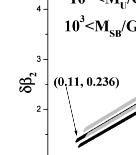
Figure 1: The allowed region of the ($\delta\beta_{1},\delta\beta_{2}$) space, for $\delta\beta_{3}=0$, in order to achieve unification in the region $10^{10}-10^{13}$ GeV, while the supersymmetry breaking is in the region $1-3$ TeV. Four different ($\alpha_{3},sin^{2}\theta_{W}$) pairs are shown.

In Fig.2 we plot the inverse of the unification coupling, $\alpha_{U}^{-1}$, versus $(\delta\beta_{1},\delta\beta_{2})$, for $\delta\beta_{3}=0$. Again, since $\alpha_{U}$ is one of the three unknowns of (12), we can easily have the required $\alpha_{U}$ for any value of $\delta\beta_{3}$. We see therefore a slight increase of the unification coupling with respect to the MSSM one ($\sim 1/24$). As far as the unification scale $M_{U}$ and the SUSY breaking scale $M_{SB}$ are concerned, there is a tendency to decrease as $\delta\beta_{1}$ gets bigger, while the opposite happens for $\delta\beta_{2}$.

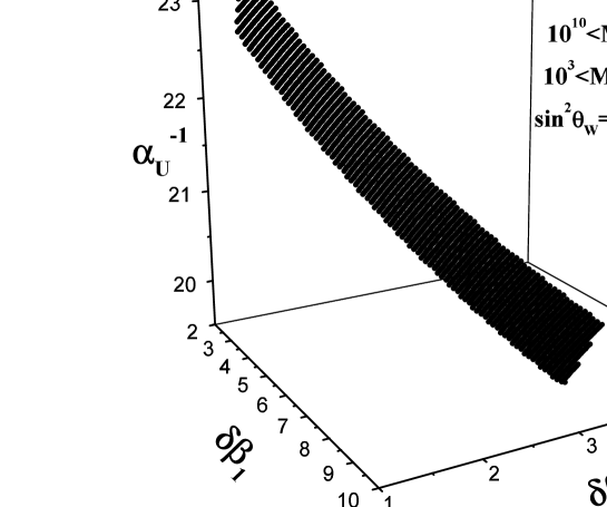
Figure 2: The inverse of the unified gauge coupling as a function of $(\delta\beta_{1},\delta\beta_{2})$, for $\delta\beta_{3}=0$ and the same constraints from $M_{U}$ and $M_{SB}$ as in Fig.1.

Let us try to find the acceptable values for a specific GUT model, namely the $SU(4)\times SU(2)_{L}\times SU(2)_{R}$. In this case, we assume that the breaking to the standard model occurs directly at the string scale $M_{I}=M_{U}$, so that the gauge couplings $g_{L},g_{R},g_{4}$ attain a common value $g_{U}$. The massless spectrum of the string model – in addition to the three families and the standard higgs fields – decomposes to the following $SU(3)\times SU(2)_{L}\times U(1)_{Y}$ representations[15]

$$n_{2} \rightarrow (1,2,\pm 1/2),\quad\quad n^{\prime}\rightarrow(1,1,\pm 1/2)$$

$$n_{3} \rightarrow (3,1,\pm 1/3),\quad\quad n_{3}^{\prime}\rightarrow(3,1,\pm 1/6)$$

$$n_{31} \rightarrow (3,1,\pm 2/3),\quad\quad n_{L}\rightarrow(1,2,0)$$

In the above, $n_{2},\,n_{3},\cdots,$ represent the number of each multiplet which appears in the corresponding parenthesis with the quantum numbers under $SU(3)\times SU(2)_{L}\times U(1)_{Y}$. In this case, the $\delta\beta_{i}$’s are given explicitly

$$\delta\beta_{1} = \frac{n_{2}}{4}+\frac{n^{\prime}}{4}+\frac{n_{3}}{3}+\frac{n_{3}^{\prime}}{12}+\frac{4}{3}n_{31}$$

$$\delta\beta_{2} = \frac{n_{2}+n_{L}}{2}$$

$$\delta\beta_{3} = \frac{n_{3}+n_{3}^{\prime}+n_{31}}{2}$$ (14)

In the specific GUT model the above $n$’s are even integers. Therefore, we see that $\delta\beta_{2,3}$ are integers while $\delta\beta_{1}$ can change by steps of $1/6$. In that case only the following 3 points are acceptable in all the region allowed by the constraints on $sin^{2}\theta_{W}(M_{Z})$ and $\alpha_{3}(M_{Z})$ having put earlier (keeping $\delta\beta_{3}=0$)

$$(\delta\beta_{1},\delta\beta_{2},\delta\beta_{3})=(4,2,0),\quad(6.5,3,0),\quad(8.5,4,0)$$

Several possible sets of $n$’s can generate the above changes in the $\beta$–functions. Again, as was mentioned above, acceptable values for higher $\delta\beta_{3}$ can be obtained in a straightforward manner

$$(4+c,2+c,c),\quad(6.5+c,3+c,c),\quad(8.5+c,4+c,c)$$

where $c$ is an integer but not any integer, since eq(12) should be satisfied for even $n^{\prime}s$. It is easy to see from these equations that we need to change $\delta\beta_{3}$ by 3 units to find an acceptable solutions for the $n^{\prime}s$

$$\begin{array}[]{cccc}(4,2,0)&(7,5,3)&(10,8,6)&...\\ (6.5,3,0)&(9.5,6,3)&(12.5,9,6)&...\\ (8.5,4,0)&(11.5,7,3)&(14.5,10,6)&...\end{array}$$ (15)

Of course, to these values correspond different sets of $n$’s and obviously as the $\delta\beta_{i}$’s increase more and more possible sets appear. We give the possible $n^{\prime}s$ for the three acceptable cases with $\delta\beta_{3}=0$

$$\begin{array}[]{||l||r|r|r||r|r|r|r||r|r|r|r|r||}\lx@intercol\hfil Table\quad 2\hfil\lx@intercol\\ \hline\cr&\lx@intercol\hfil(4,2,0)\hfil\lx@intercol\vrule\lx@intercol\vrule\lx@intercol&\lx@intercol\hfil(6.5,3,0)\hfil\lx@intercol\vrule\lx@intercol\vrule\lx@intercol&\lx@intercol\hfil(8.5,4,0)\hfil\lx@intercol\vrule\lx@intercol\vrule\lx@intercol\\ \hline\cr\hline\cr n_{2}&0&2&4&0&2&4&6&0&2&4&6&8\\ \hline\cr n_{L}&4&2&0&6&4&2&0&8&6&4&2&0\\ \hline\cr n^{\prime}&16&14&12&26&24&22&20&34&32&30&28&26\\ \hline\cr\end{array}$$ (16)

while of course $n_{3}=n_{31}=n^{\prime}_{3}=0$

We have also checked whether the radiative breaking of the electroweak symmetry is still applicable. In other words, we have used the coupled differential equation governing the running of the mass squared parameters of the scalars and checked that only $\tilde{m}^{2}_{H_{2}}$ becomes negative at a certain scale. This scale depends of course on the chosen $\delta\beta_{i}$’s, but stays in the region between $10^{5}-10^{7}$GeV.

In conclusion, we have checked the possibility of intermediate scale ($10^{10-13}$ GeV) gauge coupling unification, using the traditional logarithmic running, i.e. without incorporating the power-law dependence on the scale coming from the Kaluza-Klein tower of states. We have showed that this kind of unification can be achieved with small changes of the $\beta$-functions of the MSSM gauge couplings, which can be attributed to matter remnants of superstring models. We have applied the above to the successful $SU(4)\times SU(2)_{L}\times SU(2)_{R}$ model (which is safe against proton decay even in this intermediate scale), and found the necessary extra massless matter and higgs fields needed. Finally we have checked that the radiative electroweak breaking of the MSSM still persists, driving the mass squared of the higgs to negative values at the scale $\sim 10^{5-7}$ GeV, while all others scalar mass squared parameters stay positive.

References

[1]E. Witten, Nucl. Phys. B 471 (1996) 135.
[2]
I. Antoniadis, Phys. Lett. B 246 (1990) 377;
I.
Antoniadis, K. Benakli and M. Quiros, Phys. Lett. B 331 (1994) 313.
[3]J.D. Lykken,
Phys.Rev.D 54 (1996) 3693.
[4]
I. Antoniadis, N. Arkani-Hamed, S. Dimopoulos and G. Dvali, hep-ph/9804398;
I. Antoniadis, S. Dimopoulos, A. Pomarol and M.
Quiros, hep-ph/9810410.
[5]
K. Dienes, E. Dudas and T. Gherghetta, Phys. Lett. B 436
(1998)55; hep-ph/9806292;
D. Ghilencea and G.G. Ross, Phys.Lett.B 442 (1998) 165.
[6]
C. Bachas, hep-ph/9807415;
[7] G. Shiu and S.-H.H. Tye, Phys. Rev. D 58(1998) 106007;
Z. Kakushadze and S.H. Tye, hep-ph/9809147;
Z. Kakushadze, hep-th/9902080.
[8]
S. Abel and S.F. King, hep-ph/9809467;
K. Benakli and S. Davidson, hep-ph/9810280.
[9]N. Arkani-Hamed, S. Dimopoulos and G. Dvali, hep-ph/9807334.
[10] P. Nath and M. Yamaguchi, hep-th/9902323.
[11]C.P. Burges, L.E. Ibañez and F. Quevedo,
hep-ph/9810535.
[12]L.E. Ibañez, C. Muñoz and S. Rigolin,
hep-ph/9812397.
[13]I. Antoniadis and B. Pioline, hep-th/9902055.
[14]J. Polchinski, S. Chaudhuri and C.V. Johnson,
hep-th/9602052;
J. Polchinski, hep-th/9611050.
[15]I. Antoniadis, G.K. Leontaris and N.D. Tracas,
Phys. Lett. B 279 (1992) 58.