hep-ph/9902364 ACT-1/99 CERN-TH/99-16 CTP-TAMU-04/99 Leptogenesis in the Light of Super-Kamiokande Data and a Realistic String Model

We discuss leptogenesis in the light of indications of neutrino masses and mixings from Super-Kamiokande and other data on atmospheric neutrinos, as well as the solar neutrino deficit. Neutrino masses and mixings consistent with these data may produce in a natural and generic way a lepton asymmetry that is suffient to provide the observed baryon asymmetry, after processing via non-perturbative electroweak effects. We illustrate this discussion in the framework of the string-derived flipped $SU(5)$ model, using particle assignments and choices of vacuum parameters that are known to give realistic masses to quarks and charged leptons. We display one scenario for neutrino masses that also accommodates leptogenesis.

 

1. Intoduction

One of the basic questions in cosmology is the origin of the observed baryon asymmetry of the Universe. This could in principle have arisen either through non-perturbative effects at the electroweak phase transition [1], or via lepton- and/or baryon-number-violating interactions at high temperatures. Electroweak baryogenesis appears not to work in the Standard Model, because, e.g., of the LEP lower limit on the mass of the Higgs boson, but may be possible in its supersymmetric extensions, though these are also being constrained severely by LEP and other data. Perturbative interactions that violate lepton and/or baryon number arise naturally in grand unified extensions of the Standard Model, and baryogenesis is actually one of the main motivations for looking at these theories. So far, no baryon-number-violating interactions have yet been observed. However, it has been pointed out that leptogenesis, e.g., via the out-of-equilibrium decay of heavy Majorana neutrinos, whose masses violate lepton number, may lead to a net baryon asymmetry in the universe [2], exploiting the fact that lepton- and baryon-number-violating interactions are expected to be in thermal equilibrium at high temperatures. Within this approach [3], it is found that the asymmetries of baryon number $B$ and of $B-L$ are related by

$$Y_{B}=\left({8N_{f}+4N_{H}\over 22N_{f}+13N_{H}}\right)Y_{B-L}\,$$ (1)

where $N_{f}$ is the number of quark-lepton families and $N_{H}$ the number of Higgs doublets. This may easily yield the required baryon asymmetry $Y_{B}\equiv{n_{B}\over s}={n_{B}\over g_{*}n_{\gamma}}=\sim 10^{-10}$.

There have recently been reports from the Super-Kamiokande [4] and other [5] collaborations, indicating the existence of neutrino oscillations, for which the most natural mechanisms are neutrino masses and mixings [6, 7]. In most models, the neutrino masses are largely of Majorana type, which implies the existence of interactions that violate lepton number. Thus, the physics beyond the Standard Model that we are seeing for the first time may be just what we need to generate the baryon asymmetry of the Universe.

One intriguing feature of the atmospheric-neutrino data is that they require a large neutrino mixing angle [4, 5]. Such mixing had been shown, before the SuperKamiokande data, to arise naturally in a sub-class of GUT models [8], and more recently in certain models with flavour symmetries [9]. Moreover, it is possible [7] to accommodate the data in a natural and generic way within a flipped $SU(5)\times U(1)$ model [10] that is also consistent with the known hierarchies of charged-lepton and quark masses and mixings [11]. We showed in this analysis that flipped $SU(5)$ avoids the tight relation between $u$-quark and Dirac neutrino mass matrices found in many GUTs, and includes $SU(3)\times SU(2)\times U(1)$-singlet fields that are good candidates for $\nu_{R}$ fields. With suitable choices of the parameters of the vacuum of the string-derived flipped $SU(5)$ model, we found solutions to the atmospheric neutrino deficit with a suitable hierarchy of neutrino masses. It was possible to obtain either the small- or (perhaps preferably) the large-angle MSW solution to the solar-neutrino problem, but not the ‘just-so’ vacuum-oscillation solution.

In this paper, we re-examine scenarios for leptogenesis [2, 3] in the light of the new insights into neutrino masses and mixings provided by the Super-Kamiokande and other data. We find that leptogenesis can be successful if certain supplementary constraints on the heavy Majorana neutrino mass spectrum are obeyed. We illustrate these observations in the framework of the flipped $SU(5)$ string model, whose vacuum parameters are constrained by both the quark and charged-lepton mass hierarchies, as well as by the flat directions of the theory. We find one scenario for neutrino masses, within this general framework, that is compatible with leptogenesis.

2. Neutrino Masses, Reaction Rates and Boltzmann Equations

We consider the generic likelihood that there is a hierarchy of eigenvalues in the heavy Majorana neutrino mass matrix: $M_{N_{1}}<M_{N_{2}},M_{N_{3}}$. In such a case, the lightest right-handed neutrino will usually still be in equilibrium during the decays of the two heavier ones, therefore washing out any lepton asymmetry generated by them. For this reason, it is reasonable to assume that any lepton asymmetry is generated only by the $CP$-violating decay of the lightest right-handed neutrino $N_{1}$.

At tree level, the total decay width of $N_{1}$ is given by

$$\Gamma=\frac{(\lambda^{\dagger}\lambda)_{11}}{8\pi}M_{N_{1}}$$ (2)

where $\lambda=m^{D}_{\nu}/v$, $v$ being the corresponding light Higgs vacuum expectation value (vev). We do not assume that the Dirac neutrino couplings $\lambda$ are related directly to the $u$-quark Dirac couplings, as has often been assumed in previous works. As usual, the leading contribution to the $CP$-violating decay asymmetry, $\epsilon$, arises from the interference between the tree-level decay amplitude and one loop amplitudes. These include corrections of vertex type, but may also involve self-energy corrections $\tilde{\delta}$. The latter may even be dominant if two of the heavy neutrinos are almost degenerate [12], which can become the case in some of the examples that we study below. In general, $\epsilon$ is given by

$$\epsilon_{j} = {1\over(8\pi\lambda^{\dagger}\lambda)_{11}}\sum_{j}{\rm Im}\left[(\lambda^{\dagger}\lambda)_{1j}^{2}\right]f\left(\frac{m^{2}_{N_{j}}}{m^{2}_{N_{1}}}\right)$$ (3)

where

$$f(y) = \sqrt{y}\left[1-(1+y)\ln\left({1+y\over y}\right)\right]\;.$$ (4)

We recall that, in order to calculate consistently $CP$-violating asymmetries, lepton-number-violating scattering processes must also be included. The complete cross sections for these processes have been presented in [13], where we refer the reader for more details.

On the other hand, $\tilde{\delta}$ roughly scales as $1/\eta$, where $\eta=(M_{N_{2}}-M_{N_{1}})/M_{N_{1}}$, indicating that if the two masses are close in magnitude, but not closer than the decay widths, a large enhancement of the lepton asymmetry may occur [12]. We note, however, that when the two masses are exactly equal, the asymmetry vanishes as there is no mixing between two identical particles.

Let us define the variables $Y=n/s$ and $x=M_{N_{1}}/T$, where $n$ is the number of neutrinos per co-moving volume element, whilst $s$ is the entropy density of the Universe. The latter is given by $s=g_{*}n_{\gamma}$, where $g_{*}$ is the total number of spin degrees of freedom, and $n_{\gamma}$ is the equilibrium photon density of the Universe. We then have the following Boltzmann equation for the time evolution of the neutrino number density:

$${{\rm d}Y\over{\rm d}x}=-\frac{\Gamma(x)x}{H(x=1)}(Y-Y^{eq}),$$ (5)

where $H$ is the Hubble parameter and

$$Y^{eq}=n^{eq}/s=\left\{\begin{array}[]{ll}g_{*}^{-1}&x\ll 1\\ g_{*}^{-1}\sqrt{\pi/2}x^{3/2}\exp(-x)&x\gg 1\end{array}\right.$$ (8)

and we should impose the initial condition $Y(0)=g_{*}^{-1}$. The corresponding Boltzmann equation for the lepton asymmetry $Y_{L}$ is

$${{\rm d}Y_{L}\over{\rm d}x}=\epsilon\frac{\Gamma(x)x}{H(x=1)}(Y-Y^{eq})-g_{*}Y^{eq}Y_{L}\frac{\Gamma(x)x}{2H(x=1)}-{{2Y_{L}\Gamma_{s}x}\over H(x=1)}$$ (9)

where $\Gamma_{s}=n_{\gamma}<\sigma|v|>$, with the initial condition $Y_{L}(0)=0$. The lepton asymmetry at any time is given by solving these coupled equations. Before doing so, however, it is illuminating to see analytically what are the direct constraints on the model parameters that we can infer.

At the time of their decays, the neutrinos have to be out of equilibrium, thus the decay rate $\Gamma$ has to be smaller than the Hubble parameter $H$ at temperatures $T\approx M_{N_{1}}$. $H$ is given by

$$H\approx 1.7~{}g_{*}^{1/2}~{}\frac{T^{2}}{M_{p}}$$ (10)

where in the Minimal Supersymmetric Standard model $g_{*}\approx 228.75$, whilst $g_{*}=106.75$ for the Standard Model. This implies, as a first approximation, that

$$\frac{(\lambda^{\dagger}\lambda)_{11}}{14\pi g_{*}^{1/2}}M_{p}<M_{N_{1}}$$ (11)

However, a more accurate constraint is obtained by looking directly at the solutions of the Boltzmann equations for the system. Indeed, it turns out that even for Yukawa couplings larger than indicated in (11), the lepton-number-violating scatterings mediated by right-handed neutrinos do not wash out completely the generated lepton asymmetry at low temperatures [15]. Hence the bound on the minimal value of $M_{N_{1}}$ in terms of the Yukawa coupling is somewhat modified, as we discuss later in the analysis.

Demanding that the lepton asymmetry is generated before the electroweak phase transition gives a constraint on the lifetime of the right-handed neutrino, namely that it has to be smaller than $10^{-12}\,$s. This implies that [14]

$$(m^{D\dagger}_{\nu}m^{D}_{\nu})_{11}>\left(20\,\mbox{eV}\right)^{2}\left({10^{10}\,\mbox{GeV}\over M_{N_{1}}}\right)\;$$ (12)

which is not a very severe constraint.

In a cosmological model with inflation, one has the additional requirement that the decays of the right-handed neutrinos should occur below the scale of inflation, which is constrained by the magnitude of the density fluctuations observed by COBE. This gives

$$M_{N_{i}}\leq m_{\eta}\leq 10^{13}~{}\hbox{GeV}$$ (13)

where $m_{\eta}$ is the inflaton mass, in generic inflationary models. However, this upper limit may be increased by a couple of orders of magnitude in models with preheating [16].

Finally, one has also to take into account the likelihood that the lepton asymmetry produced in this framework is diluted by subsequent entropy production . This is discussed later in the paper.

Let us now incorporate the constraints from neutrino masses and mixings. The Super-Kamiokande as well as the solar neutrino data, which require small mass differences, can be explained by two possible neutrino hierarchies:

(a) Textures with almost degenerate neutrino mass eigenstates, of the order of ${\cal O}({\rm eV})$. In this case neutrinos may also provide a component of hot dark matter.

(b) Textures with large hierarchies of neutrino masses: $m_{\nu_{3}}\gg m_{\nu_{2}},m_{\nu_{1}}$, leaving open the possibility of a second hierarchy $m_{\nu_{2}}\gg m_{\nu_{1}}$. Then, the atmospheric neutrino data requires $m_{\nu_{3}}\approx(10^{-1}\;{\rm to}\;10^{-1.5})$ eV and $m_{\nu_{2}}\approx(10^{-2}\;{\rm to}\;10^{-3})$ eV.

This data, clearly constraints the possible mass scales of the problem. The mass of the heavier neutrino is given by

$$m_{\nu_{3}}=\frac{(m_{\nu}^{D})_{33}^{2}}{M_{N_{3}}}$$ (14)

For a scale ${\cal O}(200~{}{\rm GeV})$ for the Dirac mass, one has the following: Solutions of the type (a), that is light neutrinos of almost equal mass, require

$$M_{N_{3}}\approx{\cal O}({\rm a~{}few~{}times~{}10^{13}}~{}{\rm GeV})$$ (15)

However, given that the Dirac neutrino couplings are expected in many unified or partially unified theories to have large hierarchies (similar to those of quarks), we conclude that in order to obtain three almost degenerate neutrinos, a large hierarchy in the heavy Majorana sector would also be required. (We emphasize that this is true in the case that no reverse Dirac hierarchies are generated. An exception to this will be the example we give subsequently, where there are large entries in the 1-2 sector of the Dirac neutrino texture). In the simple case of standard neutrino Dirac hierarchies, the scale $M_{N_{1}}$ will be expected to be significantly lower than the upper bound on the inflaton mass.

On the other hand, solutions of the type (b), with large light neutrino hierarchies require

$$M_{N_{3}}\approx O({\rm a~{}few~{}times~{}10^{14}-10^{15}~{}{\rm GeV}})$$ (16)

Then, the inflaton mass condition demands heavy Majorana hierarchies of the type

$$\frac{M_{N_{1}}}{M_{N_{3}}}\leq{\cal O}\left(\frac{1}{100}\right)<\frac{M_{N_{2}}}{M_{N_{3}}}$$ (17)

The suppression of $m_{\nu_{2}}$ with respect to $m_{\nu_{3}}$ (which is roughly 1/10) can again be obtained either from the Yukawa couplings, or from the heavy Majorana mass hierarchies: For $M_{N_{2}}\approx M_{N_{3}}$ the relevant squared Yukawa couplings should have a ratio 1:10. However, for $M_{N_{2}}<M_{N_{3}}$ the ratio of the relevant squared Yukawa couplings has to be larger. The same is true for the relative suppression of $m_{\nu_{1}}$ with respect to $m_{\nu_{2}}$. Here, however, the data offers no information on how large $m_{\nu_{1}}/m_{\nu_{2}}$ can be (although the most natural expectation would be that there is a second large hierarchy). However, in case (b), $M_{N_{1}}$ can be close to the inflaton mass, unlike what happens in case (a).

It is interesting to note that leptogenesis does not allow for reverse hierarchies in the heavy Majorana mass sector, consistent with the neutrino data, even in the case that the Yukawa couplings would be close in magnitude. Indeed, the scales given by eqs. (15) and (16), in the case of reverse hierarchies, can never be consistent with the bound on the lightest heavy neutrino mass scale from the inflaton mass. At this stage it is difficult to obtain any additional information, without entering in more detail in the structure (and in particular the mixings) of the various mass matrices. This will be done in the next section, in the framework of a realistic example. However, from the above discussion it is clear that leptogenesis provides an additional probe to neutrino mass hierarchies.

At this stage, it is instructive to illustrate how the lepton asymmetry evolves in the presence of rescattering in such a scenario. In principle, one expects the following [17]: for small Dirac neutrino couplings and a large scale $M_{N_{1}}$, the scattering that tends to deplete the lepton asymmetry is suppressed. In this case, the lepton asymmetry grows to a constant asymptotic value, $Y_{asym}^{1}$. On the other hand, for larger Yukawa couplings and smaller $M_{N_{1}}$, the scattering processes start becoming relevant. Consequently, the lepton asymmetry exhibits an increase to a peak, followed by a subsequent decrease to an asymptotic value $Y_{asym}^{2}<Y_{asym}^{1}$. From the previous discussion, we see that the rough estimate of the out-of-equilibrium condition (11), for $M_{N_{1}}<10^{13}~{}{\rm GeV}$ (13), corresponds to a bound

$$(\lambda^{\dagger}\lambda)_{11}<6\cdot 10^{-4}$$ (18)

For any $(\lambda^{\dagger}\lambda)_{11}$ below this value, the lepton asymmetry grows to a constant value. However, it turns out that we may allow higher values, and still get a large enough lepton asymmetry, as is illustrated in Figure 1.

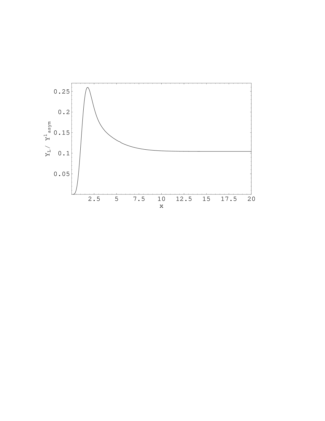
Figure 1: Evolution of lepton asymmetry for $M_{N_{1}}\approx 10^{13}$ GeV and $(\lambda^{\dagger}\lambda)_{11}=1.4\cdot 10^{-3}$.

What is the final baryon asymmetry that is generated? This is given by

$$Y_{B}\equiv\frac{n_{B}}{s}\sim\frac{n_{L}}{s}\sim\left(\frac{m_{\eta}}{M_{p}}\right)^{1/2}\frac{Y_{asym}^{2}}{Y_{asym}^{1}}~{}\frac{(\epsilon+\tilde{\delta})}{g_{*}}~{}\frac{1}{\Delta}$$ (19)

where $\Delta$ is a dilution factor, due to entropy that is produced during the breaking of $SU(5)\times U(1)$ [18] when a singlet field $\Phi$ (flaton) gets a vev. This is given by [19]

$$\Delta=\frac{s(R_{d\Phi})}{s(R_{d\eta})}(\frac{R_{d\Phi}}{R_{d\eta}})^{3}\sim\frac{V^{3}m_{\eta}^{3/2}}{{\alpha_{\Phi}}^{1/2}\ m_{SUSY}^{3/2}M_{P}^{3}}$$ (20)

In the above, the $\Phi$ decay rate is given by $\Gamma_{\Phi}=\alpha_{\Phi}\frac{m^{3}_{SUSY}}{V^{2}}$, $V$ is the scale where the vev of the Higgs ${\tt 10}$ and ${\tt\overline{10}}$ break the flipped-SU(5) group, and we take the supersymmetry breaking scale to be $m_{SUSY}\sim 10^{-16}M_{P}$. We will discuss below which is the magnitude of the dilution factor that one may accommodate in a successful scheme of leptogenesis.

3. Specialization to a Realistic Flipped $SU(5)$ String Model

As an exemplar of the above combined analysis of leptogenesis and phenomenological constraints, we consider the ‘realistic’ flipped $SU(5)$ model derived from string, working with the mass matrices discussed in [11, 7]. Relevant aspects of this model are reviewed in the Appendix: it contains many singlet fields, and the mass matrices depend on the subset of these that get non-zero vev’s, i.e., on the choice of flat direction in the effective potential. The questions we study in this section are: is the choice of vev’s made previously consistent with the cosmological constraints discussed in the previous section? and, if so: does cosmology further constrain the model parameters in an interesting way?

Within this model, we found that the charged-lepton mixing matrix is given by

$$V^{m}_{\ell_{L}}=\left(\begin{array}[]{ccc}1-\frac{1}{2}(\Delta_{2}\Delta_{5})^{2}&\Delta_{2}\Delta_{5}&0\\ -\Delta_{2}\Delta_{5}&1-\frac{1}{2}(\Delta_{2}\Delta_{5})^{2}&0\\ 0&0&1\end{array}\right)$$ (21)

where $\Delta_{2}\Delta_{5}$ is a combination of hidden-sector fields that transform as sextets under $SO(6)$ (see the Appendix for the relevant field definitions). In the same framework, $m_{\nu}^{D}$ was found to take the form

$$m_{\nu}^{D}=\left(\begin{array}[]{ccc}\Delta_{2}\Delta_{5}\overline{\phi}_{4}&1&0\\ \overline{\phi}_{4}&\Delta_{2}\Delta_{5}&0\\ 0&0&F_{1}\end{array}\right)\equiv\left(\begin{array}[]{ccc}xf&1&0\\ f&x&0\\ 0&0&y\end{array}\right)$$ (22)

where $F_{1}$ and $\overline{\phi}_{4}$ are fields also defined in the Appendix, whose vev’s are going to determine the magnitudes of the various entries. The form of the heavy Majorana mass matrix, $M_{\nu_{R}}$, is found to be

$$M_{\nu_{R}}=\left(\begin{array}[]{ccc}\overline{F}_{5}\overline{F}_{5}\overline{\phi}_{4}\phi_{3}&\overline{F}_{5}\overline{F}_{5}\Delta_{2}\Delta_{5}\phi_{3}&0\\ \overline{F}_{5}\overline{F}_{5}\Delta_{2}\Delta_{5}\phi_{3}&0&\overline{F}_{5}\overline{\Phi}_{31}\Phi_{31}\overline{\phi}_{4}\phi_{2}\\ 0&\overline{F}_{5}\overline{\Phi}_{31}\Phi_{31}\overline{\phi}_{4}\phi_{2}&\Delta_{2}\Delta_{5}\overline{\Phi}_{23}T_{2}T_{5}\end{array}\right)\equiv\left(\begin{array}[]{ccc}M&M^{\prime}&0\\ M^{\prime}&0&M_{4\phi}\\ 0&M_{4\phi}&M_{\phi\phi}\end{array}\right)$$ (23)

Using the above formulae, we were able to calculate the light-neutrino mass matrix, which is given by the standard see-saw formula:

$$m_{eff}=m^{D}_{\nu}\cdot(M_{\nu_{R}})^{-1}\cdot(m^{D}_{\nu})^{T}$$ (24)

in terms of the Dirac neutrino mass matrix $m_{\nu}^{D}$ and the heavy Majorana neutrino mass matrix $M_{\nu_{R}}$ introduced above. We note, moreover, that the mixing in the leptonic sector is given by

$$V_{\nu}=V^{m\dagger}_{\nu}V^{m}_{\ell_{L}}$$ (25)

where the symbols $V^{m}_{\nu},V_{\ell_{L}}$ denote the flavour-rotation matrices for neutrinos and left-handed charged leptons, respectively, required to diagonalize their mass matrices.

We see that, in this model, potentially large off-diagonal entries in the heavy Majorana mass matrix may yield large neutrino mixing. Moreover, the neutrino Dirac matrix, which is not equivalent to $m_{u}$ in this model, also provides a potential source of large $\nu_{\mu}-\nu_{e}$ mixing.

Clearly, the forms of the mass matrices depend on the various field vev’s. For these, we have already used information from the analysis of the flat directions and the fermion masses. We recall that our analysis of quark masses pointed towards $\Delta_{2}\Delta_{5}={\cal O}(1)$, as well as a suppressed value of $\overline{\phi}_{4}\ll 1$. Moreover, from the analysis of flat directions [11], we concluded that $\overline{\Phi}_{31}\overline{\Phi}_{23}={\cal O}(1)$ is large. In addition, the flatness conditions [11] relate $\overline{\Phi}_{31},\Phi_{31}$ and $\phi_{2}$, and can be satisfied even if all the vev’s are large, as long as $\overline{\Phi}_{31}\Phi_{31}$ and $\overline{\Phi}_{23}\Phi_{23}$ are not very close to unity. As for the decuplets that break the gauge group down to the Standard Model, we know that the vev’s should be $\approx M_{GUT}/M_{s}$. In weakly-coupled string constructions, this ratio is $\approx 0.01$. However, the strong-coupling limit of $M$ theory offers the possibility that the GUT and the string scales can coincide, in which case the vev’s could be of order unity.

On the other hand, flatness conditions and quark masses do not give any information on the vev of the product $T_{2}T_{5}$. Even this combination, however, is constrained from the requirements for the light neutrino masses [7]. Finally, the field $\phi_{3}$ is the one for which we seem to know least and we will discuss in a subsequent section how its value may affect leptogenesis.

III-A. First Class of Solutions

In [7], where we classified the flipped $SU(5)$ solutions to the super-Kamiokande data, we first considered the following simplified form for the heavy Majorana mass matrix:

$$M_{\nu_{R}}\propto\left(\begin{array}[]{ccc}M&0&0\\ 0&0&M_{4\phi}\\ 0&M_{4\phi}&M_{\phi\phi}\end{array}\right)\equiv\left(\begin{array}[]{ccc}M&0&0\\ 0&0&fy\\ 0&fy&tx\end{array}\right)$$ (32)

where our approximation was to neglect $M^{\prime}$ - but not to make any other a priori assumption about the relative magnitudes of entries in $M_{\nu_{R}}$. This approximation can be motivated if $\phi_{3}$ is negligible [11], and $M$ is eventually generated by some other effect. Then, we showed that the magnitude of $M$ is not essential for the calculations of the light neutrino data. For leptogenesis however the situation will be much different, the reason being that $M$ is directly associated with the lighter eigenvalue of the Heavy Majorana mass sector. Since $M$ essentially decouples from the rest of the entries, this is the easiest example one can calculate, since we can essentially read off the masses and Yukawa couplings that we need without explicitly calculating any mixing matrices. This will not be the case in the next section, where we will need to transform the Dirac neutrino mass matrices in the basis where the heavy Majorana one is diagonal.

We also showed that consistency within this framework, required ${\overline{F}}_{5}$ to be quite large, as could occur in the strong-coupling limit of $M$ theory. Finally, in this scheme the combination $T_{2}T_{5}$ was also fixed to be $T_{2}T_{5}\sim{\overline{\phi}}_{4}$ .

Let us now go to the Dirac mass matrix. We saw that for the calculation of the lepton asymmetry, we need to know the combination $(\lambda^{\dagger}\lambda)_{11}$. This can be read by

$$(m_{\nu}^{D\dagger}m_{\nu}^{D})\propto\left(\begin{array}[]{ccc}f^{2}(1+x^{2})&2fx&0\\ 2fx&1+x^{2}&0\\ 0&0&y^{2}\end{array}\right)$$ (36)

This indicates that $(\lambda^{\dagger}\lambda)_{11}$ is suppressed as compared to $(\lambda^{\dagger}\lambda)_{22}$ and $(\lambda^{\dagger}\lambda)_{33}$, which for strong unification are of the same order of magnitude. The eigenvalues of the heavy Majorana mass matrix are:

$$M_{N_{1}} = M$$

$$M_{N_{2}} = \frac{1}{2}(tx-\sqrt{t^{2}x^{2}+4f^{2}y^{2}})$$

$$M_{N_{3}} = \frac{1}{2}(tx+\sqrt{t^{2}x^{2}+4f^{2}y^{2}})$$ (37)

thus allowing for the possibility of a hierarchy between $M_{N_{2}}$ and $M_{N_{3}}$.

We can now use the above hierarchies, in order to estimate what would be the natural magnitude for $\epsilon$. The above Yukawa couplings and masses indicate that the dominant contribution arises from second-generation particles, in the decays of the heavy neutrinos of the first-generation. Then,

$$\epsilon_{12}\approx{1\over 8\pi}~{}\frac{(\lambda^{\dagger}\lambda)_{12}^{2}}{(\lambda^{\dagger}\lambda)_{11}}~{}f\left({M_{2}^{2}\over M_{1}^{2}}\right)~{}\delta$$ (38)

where $\delta$ is the CP-violating phase factor. Depending how close $M_{2}$ is to $M_{1}$, $\epsilon$ may be as large as $10^{-2}\delta$ . On the other hand, $\tilde{\delta}$ may be significantly enhanced for $M_{1}\approx M_{2}$, although for large mass differences it is of the same order as $\epsilon$.

Finally, we need to calculate the ratio $(Y_{asymm}^{2}/Y_{asymm}^{1})$ from the Boltzmann equations and for $(\lambda^{\dagger}\lambda)_{11}\approx f^{2}\approx 0.0016$ (where we stress again that we neglect coefficients of order unity, which are currently not predicted by the theory). It turns out that, for $M_{N_{1}}=10^{13}~{}{\rm GeV}$,

$$\frac{Y_{asymm}^{2}}{Y_{asymm}^{1}}=9\cdot 10^{-2}$$ (39)

whilst, for $M_{N_{1}}=10^{11}~{}{\rm GeV}$,

$$\frac{Y_{asymm}^{2}}{Y_{asymm}^{1}}=4\cdot 10^{-4}$$ (40)

We see therefore that by lowering $M_{N_{1}}$ while keeping the Yukawa coupling fixed, we significantly lower the produced lepton asymmetry. However, remember that a higher value of $M_{N_{1}}$ also requires a higher inflaton mass and then the dilution factor $\Delta$ becomes larger.

We see, then, that (even in the case that $M_{N_{1}}$ and $M_{N_{2}}$, while being close in magnitude, do not fulfil the resonant condition that increases the generated asymmetry) $M_{N_{1}}=10^{13}$ GeV yields a ratio

$$Y_{B}\equiv\frac{n_{B}}{s}\approx~{}\frac{3\cdot 10^{-8}}{\Delta}$$ (41)

which can be in the acceptable range $Y_{B}^{observed}\approx 10^{-10}$ for $\Delta\leq 300$. This is difficult to reconcile with (20), but might be consistent with suitably large $\alpha_{\Phi}$ and $m_{SUSY}$. 

Moreover, note that the various entries in the mass matrices, are only known up to order unity coefficients, while a small change in a Yukawa coupling can have a large effect on the ratio $(Y_{asymm}^{2}/Y_{asymm}^{1})$. Indeed, for $M_{N_{1}}=10^{13}$ GeV, one has the following: for $(\lambda^{\dagger}\lambda)_{11}=0.001$,

$$\frac{Y_{asymm}^{2}}{Y_{asymm}^{1}}=0.16$$ (42)

whilst, for $(\lambda^{\dagger}\lambda)_{11}=0.0004$,

$$\frac{Y_{asymm}^{2}}{Y_{asymm}^{1}}=0.45$$ (43)

Finally, we recall that in the presence of preheating, one may raise the limit on the inflaton mass, and hence the value of $Y_{asymm}^{2}/Y_{asymm}^{1}$. For example, if $M_{N_{1}}=10^{14}$ GeV and $(\lambda^{\dagger}\lambda)_{11}=0.001$, we find

$$\frac{Y_{asymm}^{2}}{Y_{asymm}^{1}}=0.86$$ (44)

However, since

$$Y_{B}~{}\propto~{}\frac{1}{\Delta}\left(\frac{m_{\eta}}{M_{p}}\right)^{1/2}\sim\frac{1}{m_{\eta}}$$ (45)

by raising the limit on the inflaton mass and thus the possible mass for the lighter neutrino, we end up with a larger suppression due to entropy production.

III-B. Second Class of Solutions

We will now investigate whether our parametrization of the flipped $SU(5)$ model matches the cosmological requirements, for the second class of solutions that we found in [7]. These occur in the case that the field $\phi_{3}$ develops a large vev. Previously, we had assumed for simplicity that $\phi_{3}\approx 1$. This is actually the most natural range, given that large $\phi_{3}$ allows for a suppression of $m_{\nu_{e}}$ and $m_{\nu_{\mu}}$ as compared to $m_{\nu_{\tau}}$. Then, we can write $M_{\nu_{R}}$ in the form

$$M_{\nu_{R}}\propto\left(\begin{array}[]{ccc}fy^{2}&2xy^{2}&0\\ 2xy^{2}&0&fy\\ 0&fy&tx\end{array}\right)$$ (46)

where $\Delta_{2}\Delta_{5}\equiv x,T_{2}T_{5}\equiv t$, $\overline{\phi}_{4}\equiv f$ and $\overline{F}_{5}\equiv y$. In the above, the factor of $2$ has been included in order to avoid sub-determinant cancellations, which are not expected to arise once order unity coefficients are properly taken into account.

Let us then write down $m_{eff}$ in the flipped-$SU(5)$ field basis. This is given by

$$m_{eff}\propto\left(\begin{array}[]{ccc}-f^{4}x^{2}+tfx&-f^{4}x-tfx^{2}&-f^{2}y^{2}\\ -f^{4}x-tfx^{2}&-f^{4}-3ftx^{3}&f^{2}xy^{2}\\ -f^{2}y^{2}&f^{2}xy^{2}&-4x^{2}y^{4}\end{array}\right)$$ (50)

As we see from this matrix (and have stressed in our previous analysis), the neutrino data solutions with large light neutrino hierarchies require $\overline{\phi}_{4}\approx\overline{F}_{5},F_{1}$, as in weak-coupling unification schemes [7]. On the other hand, $T_{2}T_{5}$ is not fixed to a specific value, however it has to be smaller than $(\overline{\phi}_{4})^{3}$, so that the entries in the (1,2) sector of $m_{eff}$ remain small. Here we should stress that ${\cal O}{\rm(1)}$ coefficients may not be fixed by the model and therefore we are only concerned with the order of magnitude of the various entries, as it is specified by the operators.

Finally, the Dirac mass matrix, is similar to the one calculated before, with the difference that $y$ is now much smaller. In this example, the light Majorana mass matrix does not decouple and therefore in order to work with the $M_{N_{i}}$ mass eigenstates, we need to diagonalise $M_{\nu_{R}}$ and also transform $m_{\nu}^{D}$ to the basis where $M_{\nu_{R}}$ is diagonal. Indeed, let

$$M_{\nu_{R}}^{diag}=V^{T}\cdot M_{\nu_{R}}\cdot V$$ (51)

Then the Yukawa couplings have to be calculated from the matrix

$$\tilde{m}_{\nu}^{D}~{}=~{}{m}_{\nu}^{D}\cdot V$$ (52)

Since in this class of solutions we require $x\approx 1,y\approx f$ and $t\leq f^{3}$, we can express the solutions only in terms of the parameter $f$. Let us first calculate the eigenvalues of the heavy Majorana mass matrix. For the particular choice of coefficients that appear in eq.(46), these scale as $f^{3}/5:\sqrt{5}f^{2}:-\sqrt{5}f^{2}$. Note here that the coefficients are not so relevant, since we do not have any information about $O(1)$ factors from the model; given that a small difference in a mass entry may lead to a significantly larger factor in the eigenvalues, we see that there is some room for arbitrariness. What is unambiguous however, is that in this class of solutions, the lightest eigenvalue tends to be suppressed as to the heavier ones, by a factor of $f\approx 0.04$, while the two heavier eigenvalues are of almost equal magnitude.

The mixing matrix, again for the coefficient choice of eq.(46) and keeping only the dominant contributions is given by

$$V=\left(\begin{array}[]{ccc}0.63&0.63&-0.45\\ 0.70&-0.70&0.18~{}f\\ 0.32&0.32&0.89\end{array}\right)$$ (56)

where we see that in this example, almost all the dominant entries of the mixing matrix are of order unity. This was to be expected, since the dominant entries in $M_{\nu_{R}}$ are the off-diagonal ones. Of course, the exact value of the mixing depends on unknown coefficients, however since it is nearly maximal, suppression factors of the order of $\sqrt{2}/2\approx 0.70$ arise in any case.

The above discussion implies that the large off-diagonal factors in $m_{\nu}^{D}$ will start getting communicated in the diagonal ones. Indeed (for $x\approx 1,y\approx f$),

$$\tilde{m}_{\nu}^{D}~{}\approx~{}\left(\begin{array}[]{rrr}0.70&-0.70&-0.27f\\ 0.70&-0.70&-0.27f\\ 0.32f&0.32f&0.9f\end{array}\right)$$ (60)

and therefore

$$\tilde{m}_{\nu}^{D\dagger}\tilde{m}_{\nu}^{D}=\left(\begin{array}[]{ccc}1&-1&-0.4f\\ -1&1&0.4f\\ -0.4f&0.4f&0.9f^{2}\end{array}\right)$$ (64)

thus indicating a significant increase in $(\lambda^{\dagger}\lambda)_{11}$ , a small decrease in $(\lambda^{\dagger}\lambda)_{22}$ and a larger decrease in $(\lambda^{\dagger}\lambda)_{33}$, which are in the wrong direction for leptogenesis. This combined with the suppression of the second lightest eigenvalue with respect to the lighter one, which reduces the value of $\epsilon$ and thus of $Y_{B}$ by a factor of $\approx 0.04$, seems to make this case not viable.

Suppose now that we leave the field $\phi_{3}$ as a free parameter. Then, the heavy Majorana mass matrix becomes of the form

$$M_{\nu_{R}}\propto\left(\begin{array}[]{ccc}fy^{2}\phi_{3}&2xy^{2}\phi_{3}&0\\ 2xy^{2}\phi_{3}&0&fy\\ 0&fy&tx\end{array}\right)$$ (65)

and the light effective one

$$m_{eff}\propto\left(\begin{array}[]{ccc}-f^{4}x^{2}+tfx\phi_{3}&-f^{4}x-tfx^{2}\phi_{3}&-f^{2}y^{2}\phi_{3}\\ -f^{4}x-tfx^{2}\phi_{3}&-f^{4}-3ftx^{3}\phi_{3}&f^{2}xy^{2}\phi_{3}\\ -f^{2}y^{2}\phi_{3}&f^{2}xy^{2}\phi_{3}&-4x^{2}y^{4}\phi_{3}^{2}\end{array}\right)$$ (69)

Then, we see that viable neutrino hierarchies are also obtained for strong unification $(y\approx 1)$ and $\phi_{3}\approx f^{2}$. The eigenvalues of $m_{\nu_{R}}$ scale as $f^{2}:1:-1$, while the mixing matrix is now

$$V=\left(\begin{array}[]{ccc}0&0&-1\\ 0.7&-0.7&0\\ 0.7&0.7&2f\end{array}\right)$$ (73)

Then (for $x,y\approx 1$)

$$\tilde{m}_{\nu}^{D}~{}\approx~{}\left(\begin{array}[]{ccc}0.7&-0.7&-f\\ 0.7&-0.7&-f\\ 0.7&0.7&2f\end{array}\right)$$ (77)

and

$$\tilde{m}_{\nu}^{D\dagger}\tilde{m}_{\nu}^{D}=\left(\begin{array}[]{ccc}1.5&-0.5&0\\ -0.5&1.5&3f\\ 0&3f&6f^{2}\end{array}\right)$$ (81)

indicating that in this limit of field vevs as well, the coupling $(\lambda^{\dagger}\lambda)_{11}$ is large, thus not allowing the fulfilment of the out-of-equilibrium condition.

4. Conclusions

In this paper, we have revisited leptogenesis in the light of the indications from Super-Kamiokande [4] and other data [5] for non-zero neutrino masses. These data provide significant additional constraints on scenarios for leptogenesis [2, 3], in particular on the possible magnitudes of heavy Majorana masses and on the possible patterns of mixing. We have shown that a plausible framework for leptogenesis is compatible with these new experimental constraints.

Our discussion has been illustrated by examples derived from a flipped $SU(5)$ string model for quark and charged-lepton masses [11], which we extended recently [7] to models of neutrino masses that were compatible with the Super-Kamiokande and other data. We have shown that one of the neutrino-mass models proposed previously leads to an acceptable realization of leptogenesis, whilst the other has problems. This analysis exemplifies the power of leptogenesis to refine further the selection of realistic models. We consider it a non-trivial success of flipped $SU(5)$ that it may survive this new set of constraints.

The more general message for model-builders that we extract from this analysis is that one must be wary about the couplings between the first generation and the other two. If there is a large off-diagonal Dirac-type Yukawa coupling, as may arise in flipped $SU(5)$, the mixing between the first-generation and other heavy Majorana masses is constrained. The emerging pattern of light neutrino masses suggests that the first and other two generations may have substantial mixing, which could arise a priori from either the Dirac and/or the heavy Majorana sectors. Our analysis suggests that leptogenesis may be unhealthy if one combines the two sources of mixing. The essential reason for this is the out-of-equilibrium condition on the neutrino couplings.

Acknowledgements

The work of D.V.N. has been supported in part by the U.S. Department of Energy under grant DE-FG03-95-ER-40917.

Appendix

In this appendix we tabulate for completeness the field assignment of the ‘realistic’ flipped $SU(5)$ string model [10], as well as the basic conditions used in [11] to obtain consistent flatness conditions and acceptable Higgs masses.

$F_{1}(10,\frac{1}{2},-\frac{1}{2},0,0,0)$	$\overline{f}_{1}(\overline{5},-\frac{3}{2},-\frac{1}{2},0,0,0)$	$\ell_{1}^{c}(1,\frac{5}{2},-\frac{1}{2},0,0,0)$
$F_{2}(10,\frac{1}{2},0,-\frac{1}{2},0,0)$	$\overline{f}_{2}(\overline{5},-\frac{3}{2},0,-\frac{1}{2},0,0)$	$\ell_{2}^{c}(1,\frac{5}{2},0,-\frac{1}{2},0,0)$
$F_{3}(10,\frac{1}{2},0,0,\frac{1}{2},-\frac{1}{2})$	$\overline{f}_{3}(\overline{5},-\frac{3}{2},0,0,\frac{1}{2},\frac{1}{2})$	$\ell_{3}^{c}(1,\frac{5}{2},0,0,\frac{1}{2},\frac{1}{2})$
$F_{4}(10,\frac{1}{2},-\frac{1}{2},0,0,0)$	$f_{4}(5,\frac{3}{2},\frac{1}{2},0,0,0)$	$\overline{\ell}_{4}^{c}(1,-\frac{5}{2},\frac{1}{2},0,0,0)$
$\overline{F}_{5}(\overline{10},-\frac{1}{2},0,\frac{1}{2},0,0)$	$\overline{f}_{5}(\overline{5},-\frac{3}{2},0,-\frac{1}{2},0,0)$	$\ell_{5}^{c}(1,\frac{5}{2},0,-\frac{1}{2},0,0)$

$h_{1}(5,-1,1,0,0,0)$	$h_{2}(5,-1,0,1,0,0)$	$h_{3}(5,-1,0,0,1,0)$
$h_{45}(5,-1,-\frac{1}{2},-\frac{1}{2},0,0)$

$\phi_{45}(1,0,\frac{1}{2},\frac{1}{2},1,0)$	$\phi_{+}(1,0,\frac{1}{2},-\frac{1}{2},0,1)$	$\phi_{-}(1,0,\frac{1}{2},-\frac{1}{2},0,-1)$
$\Phi_{23}(1,0,0,-1,1,0)$	$\Phi_{31}(1,0,1,0,-1,0)$	$\Phi_{12}(1,0,-1,1,0,0)$
$\phi(1,0,\frac{1}{2},-\frac{1}{2},0,0)$	$\Phi(1,0,0,0,0,0)$

$\Delta_{1}(0,1,6,0,-\frac{1}{2},\frac{1}{2},0)$	$\Delta_{2}(0,1,6,-\frac{1}{2},0,\frac{1}{2},0)$	$\Delta_{3}(0,1,6,-\frac{1}{2},-\frac{1}{2},0,\frac{1}{2})$
$\Delta_{4}(0,1,6,0,-\frac{1}{2},\frac{1}{2},0)$	$\Delta_{5}(0,1,6,\frac{1}{2},0,-\frac{1}{2},0)$

$T_{1}(0,10,1,0,-\frac{1}{2},\frac{1}{2},0)$	$T_{2}(0,10,1,-\frac{1}{2},0,\frac{1}{2},0)$	$T_{3}(0,10,1,-\frac{1}{2},-\frac{1}{2},0,\frac{1}{2})$
$T_{4}(0,10,1,0,\frac{1}{2},-\frac{1}{2},0)$	$T_{5}(0,10,1,-\frac{1}{2},0,\frac{1}{2},0)$

Table 3: The chiral superfields are listed with their quantum numbers [10]. The $F_{i}$, $\overline{f}_{i}$, $\ell_{i}^{c}$, as well as the $h_{i}$, $h_{ij}$ fields and the singlets are listed with their $SU(5)\times U(1)^{\prime}\times U(1)^{4}$ quantum numbers. Conjugate fields have opposite $U(1)^{\prime}\times U(1)^{4}$ quantum numbers. The fields $\Delta_{i}$ and $T_{i}$ are tabulated in terms of their $U(1)^{\prime}\times SO(10)\times SO(6)\times U(1)^{4}$ quantum numbers.

As can be seen, the matter and Higgs fields in this string model carry additional charges under additional $U(1)$ symmetries [10]. There exist various singlet fields, and hidden-sector matter fields which transform non-trivially under the $SU(4)\times SO(10)$ gauge symmetry, some as sextets under $SU(4)$, namely $\Delta_{1,2,3,4,5}$, and some as decuplets under $SO(10)$, namely $T_{1,2,3,4,5}$. There are also quadruplets of the $SU(4)$ hidden symmetry which possess fractional charges. However, these are confined and will not concern us further.

The usual flavour assignments of the light Standard Model particles in this model are as follows:

$$\overline{f}_{1}:\overline{u},\tau,\;\;\;\overline{f}_{2}:\overline{c},e/\mu,\;\;\;\overline{f}_{5}:\overline{t},\mu/e$$

$$F_{2}:Q_{2},\overline{s},\;\;\;F_{3}:Q_{1},\overline{d},\;\;\;F_{4}:Q_{3},\overline{b}$$

$$\ell^{c}_{1}:\overline{\tau},\;\;\;\ell^{c}_{2}:\overline{e},\;\;\;\ell^{c}_{5}:\overline{\mu}$$ (82)

up to mixing effects, which are discussed in more detail in [11]. We chose non-zero vacuum expectation values for the following singlet and hidden-sector fields:

$$\Phi_{31},\overline{\Phi}_{31},\Phi_{23},\overline{\Phi}_{23},\phi_{2},\overline{\phi}_{3,4},\phi^{-},\overline{\phi}^{+},\phi_{45},\overline{\phi}_{45},\Delta_{2,3,5},T_{2,4,5}$$ (83)

The vacuum expectation values of the hidden-sector fields must satisfy the additional constraints

$$T_{3,4,5}^{2}=T_{i}\cdot T_{4}=0,\,\,\Delta_{3,5}^{2}=0,\,\,T_{2}^{2}+\Delta_{2}^{2}=0$$ (84)

For further discussion, see [11] and references therein.

References

- [1] V.A. Kuzmin, V.A. Rubakov and M.E. Shaposhnikov, Phys. Lett. B155 (1985) 36.
- [2] M. Fukugita and T. Yanagida, Phys. Lett. B174 (1986) 45.
- [3] For a review on heavy Majorana neutrinos and baryogenesis, see, e.g., A. Pilaftsis, hep-ph/9812256 and references therein.
- [4] Y. Fukuda et al., Super-Kamiokande collaboration, hep-ex/9803006, hep-ex/9805006; hep-ex/9807003.
- [5] S. Hatakeyama et al., Kamiokande collaboration, hep-ex/9806038; M. Ambrosio et al., MACRO collaboration, hep-ex/9807005; M. Spurio, for the MACRO collaboration, hep-ex/9808001; W.W.M. Allison et al., Soudan-2 Collaboration, hep-ex/9901024.
- [6] For recent work, see for example: A. Joshipura and A. Smirnov, Phys. Lett. B439 (1998) 103; V. Barger, S.Pakvasa, T.J. Weiler and K. Whisnant, Phys. Lett. B437 (1998) 107; S.F. King, Phys. Lett. B439 (1998) 350; B.C. Allanach, hep-ph/9806294; R. Barbieri, L.J. Hall, D. Smith, A. Strumia and N. Weiner, hep-ph/9807235; G. Lazarides and N. Vlachos, Phys. Lett. B441 (1998) 46; M. Tanimoto, Phys. Rev. D59 (1999) 017304; M. Gonzalez-Garcia, H. Nunokawa, O.L.G. Perez and J.W.F. Valle, hep-ph/9807305; M. Jezabek and Y. Sumino, Phys. Lett. B440 (1998) 327; J. Pati, hep-ph/9807315; V. Barger, T. Weiler and K. Whisnant, Phys. Lett. B440 (1998) 1; G. Altarelli and F. Feruglio, Phys. Lett. B439 (1998) 112; JHEP 9811 (1998) 021; hep-ph/9812475. E. Ma, Phys. Lett. B442 (1998) 238; S. M. Bilenky, C. Giunti and W. Grimus, hep-ph/9812360; G.L. Fogli, E. Lisi, A. Marrone and G. Scioscia, Phys. Rev. D59 (1999) 033001; S. Davidson and S. King, Phys. Lett. B445 (1998) 191; R. Barbieri, L.J. Hall and A. Strumia, hep-ph/9808333; V. Barger, S. Pakvasa, T.J. Weiler, K. Whisnant, Phys. Rev. D58 (1998) 093016; C.H. Albright and S.M. Barr, Phys. Rev. D58 (1998) 013002; J. K. Elwood, N. Irges and P. Ramond, Phys. Rev. Lett. 81 (1998) 5064; M. Fukugita, M. Taminoto and T. Yanagida, hep-ph/9809554; W. Buchmuller and T. Yanagida, hep-ph/9810308; Y. Grossman, Y. Nir and Y. Shadmi, JHEP 9810 (1998) 007; C.D. Froggatt, M. Gibson and H.B. Nielsen, hep-ph/9811265; Q. Shafi and Z. Tavartkiladze, hep-ph/9811282; Z. Berezhiani and A. Rossi, hep-ph/9811447; C. Wetterich, hep-ph/9812426; R. Barbieri, L.J. Hall, G.L. Kane and G.G. Ross, hep-ph/9901228; S. Lola and G.G. Ross, hep-ph/9902283.
- [7] J. Ellis, G.K. Leontaris, S. Lola and D.V. Nanopoulos, hep-ph/9808251, to appear in Eur. Jour. Phys. C.
- [8] G.K. Leontaris and D.V. Nanopoulos, Phys. Lett. B212 (1988) 327.
- [9] H. Dreiner, G.K. Leontaris, S. Lola, G.G. Ross and C. Scheich, Nucl. Phys. B436 (1995) 461; G.K. Leontaris, S. Lola and G.G. Ross, Nucl. Phys. B454 (1995) 25; G.K. Leontaris, S. Lola, C. Scheich and J. Vergados, Phys. Rev. D 53 (1996) 6381; P. Binetruy, S. Lavignac and P. Ramond, Nucl. Phys. B477 (1996) 353; Y. Grossman and Y. Nir, Nucl. Phys. B448 (1995) 30; B.C. Allanach and S.F. King, Nucl.Phys. B459 (1996) 75; S. Lola and J. Vergados, Progress in Particle and Nuclear Physics 40 (1998) 71; Y. Achiman and T. Greiner, Nucl. Phys. B443 (1995) 3; P. Binetruy, S. Lavignac, S. Petcov and P. Ramond, Nucl. Phys. B496 (1997) 3.
- [10] I. Antoniadis, J. Ellis, J. Hagelin and D.V. Nanopoulos, Phys. Lett. B194 (1987) 231; Phys. Lett. B231 (1989) 65.
- [11] J. Ellis, G.K. Leontaris, S. Lola and D.V. Nanopoulos, Phys. Lett. B425 (1998) 86.
- [12] M. Flanz, E.A. Paschos and U. Sarkar, Phys. Lett. B345 (1995) 248; M. Flanz, E.A. Paschos, U. Sarkar and J. Weiss, Phys. Lett. B389 (1996) 693; L. Covi and E. Roulet, Phys. Lett. B399 (1997) 113; A. Pilaftsis, Phys. Rev. D56 (1997) 5431.
- [13] M.A. Luty, Phys. Rev. D45 (1992) 455.
- [14] M. Plumacher, Z. Phys. C74 (1997) 549.
- [15] E.W. Kolb and M.S. Turner, The Early Universe, Frontiers in Physics by Addison-Wesley publishing company.
- [16] L. Kofman, A. Linde and A. A. Starobinsky, Phys. Rev. Lett. 76 (1996) 1011; I.I. Tkachev, Phys. Lett. B376 (1996) 35; G.W. Anderson, A. Linde and A. Riotto, Phys. Rev. Lett. 77 (1996) 3716; E.W. Kolb, A. Linde and A. Riotto, Phys. Rev. Lett. 77 (1996) 4290.
- [17] See for example: M.A. Luty [13]; W. Buchmuller and M. Plumacher, Phys. Lett. B389 (1996) 73; J. Faridani, S. Lola, P.O’ Donnell and U. Sarkar, hep-ph/9804261, to appear in the Eur. Jour. Phys. C; M. Flanz and E.A. Paschos, Phys. Rev. D58 (1998) 113009.
- [18] B. Campbell, J. Ellis, J.Hagelin, D.V. Nanopoulos and K.A. Olive, Phys. Lett. B197 (1987) 355.
- [19] J. Ellis, D.V. Nanopoulos and K. Olive, Phys. Lett. B300 (1993) 121.