Hide and Seek with Supersymmetry

Abstract

This is the summary of a 90 minute introductory talk on Supersymmetry presented at the August 1998 Zuoz Summer School on “Hidden Symmetries and Higgs Phenomena”. I first review the hierarchy problem, and then discuss why we expect supersymmetry just around the corner, i.e. at or below $1\,TeV$. I focus on the specific example of the anomalous magnetic moment of the muon to show how supersymmetry can indeed hide just around the corner without already having been detected. An essential part of supersymmetry’s disguise is the fact that it is broken. I end by briefly outlining how the disguise itself is also hidden.

1 Introduction

In the Standard Model (SM), $SU(2)_{L}$ transformations relate the components of multiplets

$$T^{a}:\quad e^{-}_{L}\longleftrightarrow\nu_{e}.$$ (1)

Here $T^{a}$ is the $SU(2)_{L}$ isospin-one, bosonic generator, which changes $SU(2)_{L}$ isospin. In supersymmetry the transformations relate particles of different spin

$$Q_{\alpha}:\quad e^{-}_{L}(s=\frac{1}{2})\longleftrightarrow{\tilde{e}}^{-}_{L}(s=0),$$ (2)

in this case the left-handed electron and the left-handed scalar electron (selectron). Here $Q_{\alpha}$ is a spinorial generator, a 2-component, spin-$1/2$, Weyl-spinor, which transforms as a left-handed spinor under the Lorentz group. $\alpha=1,2$ is the spinor index. $Q_{\alpha}$ changes the spin and hence it must have a non-trivial algebra with the Lorentz-group.

$$[P^{\mu},Q_{\alpha}] = 0,$$ (3)

$$\left[M^{\mu\nu},Q_{\alpha}\right] = -i(\sigma^{\mu\nu})_{\alpha}^{\beta}Q_{\beta},$$ (4)

$$\{Q_{\alpha},Q_{\beta}\}=\{{\overline{Q}}_{\dot{\alpha}},{\overline{Q}}_{\dot{\beta}}\} = 0,$$ (5)

$$\{Q_{\alpha},{\overline{Q}}_{\dot{\beta}}\} = 2\sigma_{\alpha\dot{\beta}}^{\mu}P_{\mu}.$$ (6)

Here $\sigma^{\mu}=(\bf{1},\sigma^{i})$ and $\sigma^{i}$ are the Pauli matrices. ${\overline{\sigma}}^{\mu}=(\bf{1},-\sigma^{i})$ and $\sigma^{\mu\nu}=\frac{1}{4}({\sigma}^{\mu}{\overline{\sigma}}^{\nu}-{\sigma}^{\nu}{\overline{\sigma}}^{\mu})$. $P^{\mu}$ is the energy-momentum tensor and $M^{\mu\nu}$ is the angular momentum tensor. Since $Q_{\alpha}$ has spin and thus angular momentum the commutator with $M^{\mu\nu}$ is non-trivial. The dotted spinorial indices, e.g. $\dot{\beta}$, transform as a right-handed spinors under the Lorentz group.

From the algebra we can immediately derive some simple consequences.

• From Eq.(5) and Eq.(6) it follows that $Q_{\alpha}$ is a raising operator and ${\overline{Q}}_{\dot{\beta}}$ is a lowering operator. Since $Q_{\alpha}Q_{\alpha}=0$ (no summation) by Eq.(5) we only have two components to a supermultiplet

  $$\{{\tilde{e}}^{-}_{L}\;(s=0);e_{L}^{-}\;(s=\frac{1}{2})\},\quad\{{\tilde{e}}^{-}_{R}\;(s=0);e_{R}^{-}\;(s=\frac{1}{2})\},\quad\{\lambda_{\tilde{\gamma}}\;(s=\frac{1}{2});\gamma\;(s=1)\}.$$ (7)

  And each multiplet has equal numbers of bosonic and fermionic degrees of freedom.

• From Eq.(3) we have $[P\cdot P,Q_{\alpha}]=0$ and thus $[M^{2},Q_{\alpha}]=0$, where $M$ is the mass of the field. If supersymmetry is conserved

  $$M({\tilde{e}}^{-})=M(e^{-})=511\,KeV,\quad M({\tilde{\gamma}}^{-})=M(\gamma)=0.$$ (8)

  No charged scalar has been observed up to LEP2 energies, which are significantly higher than $M(e^{-})$. We therefore conclude that supersymmetry must be broken.

These two points can be summarized into one formula [2]

$$STr{\cal M}^{2} = 0,$$ (9)

$$STr({\cal M}^{2}) \equiv \sum_{i}(-1)^{2S_{i}}\cdot(2S_{i}+1)\,M_{i}^{2}.$$ (10)

$STr({\cal M}^{2})$ is the supertrace of the mass matrix squared containing fields of different spin, $S_{i}$. For just the electron supermultiplet, we have

$$STr({\cal M}^{2})=M_{{\tilde{e}}_{L}}^{2}+M_{{\tilde{e}}_{R}}^{2}-2M_{e}^{2}=0,\qquad\Longrightarrow\quad\frac{M_{{\tilde{e}}_{L}}^{2}+M_{{\tilde{e}}_{R}}^{2}}{2}=M_{e}^{2}$$ (11)

This is a catastrophe. At least one of the selectron fields must have mass less than or equal to $M_{e}$, which is excluded by experiment. It turns out that, Eq.(10) is also true if global supersymmetry is spontaneously broken, as we show in Sect.7. Therefore, just breaking supersymmetry does not solve this problem of the spectrum. However, the supertrace formula need only apply to the full set of fields. Thus, one might think a heavy selectron can be compensated by a higgsino or gaugino which has opposite sign. It has proven impossible to construct such models and we shall come to this problem again in Sect.7.

2 Motivation for Supersymmetry

To date there is no experimental evidence for supersymmetry. All the same it is an intensely studied subject. Why? We first give an aesthetic argument, which however tells you nothing about the scale of supersymmetry breaking. Next we discuss the hierarchy problem which indicates that supersymmetry is broken near the electroweak scale.

2.1 Unique Extension of the Symmetries of the S-Matrix

The S-matrix in the Standard Model has external and internal symmetries. The Lorentz invariance is a space-time symmetry and thus an external symmetry. The gauge symmetry $G_{SM}=SU(3)\times SU(2)\times U(1)$ and the global baryon- and lepton-number invariance are internal symmetries whose generators commute with the Lorentz generators. The following remarkable theorem holds [3, 4]: Supersymmetry is the only possible external symmetry of the S-matrix, beyond the Lorentz symmetry, for which the S-matrix is not trivial. It is beyond the scope of this lecture to present a formal proof. Instead, I give a heuristic argument which hopefully makes the theorem at least plausible [5].

Figure 1: Spinless $2\rightarrow 2$ scattering. The $p_{i}$ label the momenta of the particles.

Consider spin-less $2\rightarrow 2$ scattering as shown in Fig. 1. The incoming four-momenta are labelled by $p_{1},\,p_{2}$ and the outgoing four-momenta by $p_{3},\,p_{4}$. Momentum conservation (Lorentz symmetry) implies $p_{1}+p_{2}=p_{3}+p_{4}$. For simplicity, we shall assume the particles have equal mass $p_{i}^{2}=m_{i}^{2}=m^{2}$. The argument below also holds for more general masses. The scattering amplitude is a Lorentz scalar. It can thus only depend on the Lorentz invariants of the scattering process. The most common choice of these invariants are the Mandelstam variables

$$s=(p_{1}+p_{2})^{2},\quad t=(p_{1}-p_{3})^{2},\quad u=(p_{2}-p_{3})^{2}.$$ (12)

Since $s+t+u=4m^{2}$, only two of the invariants are independent. We choose the centre-of-mass energy squared, $s$, and the scattering angle $\cos\theta=1-2t/(s-4m^{2})$ in the centre-of-mass system.

According to the Coleman-Mandula theorem [3], if we add any further external symmetry to our theory, whose generators are tensors, then the scattering process must be trivial, i.e. there is no scattering at all. Consider the following example. Assume the tensor $R^{\mu\nu}=p^{\mu}p^{\nu}-\frac{1}{4}g^{\mu\nu}m^{2}$, is conserved, where $\mu,\nu=1,\ldots,4$ are Lorentz vector indices. Then

$$R_{1}^{\mu\nu}+R_{2}^{\mu\nu} = R_{3}^{\mu\nu}+R_{4}^{\mu\nu},$$ (13)

$$\Longrightarrow\quad p_{1}^{\mu}p_{1}^{\nu}+p_{2}^{\mu}p_{2}^{\nu} = p_{3}^{\mu}p_{3}^{\nu}+p_{4}^{\mu}p_{4}^{\nu}.$$ (14)

In the centre-of-mass coordinate system we have

$$\begin{array}[]{ll}p_{1}=(E,0,0,p),&p_{2}=(E,0,0,-p),\\ p_{3}=(E,0,p\sin\theta,p\cos\theta),&p_{4}=(E,0,-p\sin\theta,-p\cos\theta).\end{array}$$ (15)

The conservation of $R^{\mu\nu}$ (14) then implies for $\mu=\nu=4$

$$2p^{2}=2p^{2}\cos^{2}\theta,\quad\Longrightarrow\quad\theta=0.$$ (16)

There is thus no scattering at all if $R^{\mu\nu}$ is conserved. The more general statement is that it any new conserved external tensor leads to trivial scattering.

Coleman and Mandula [3] showed that the only possible conserved quantities that transform as tensors under the Lorentz group are the generators of the Poincaré group $P_{\mu},\,M_{\mu\nu}$ and Lorentz scalars $C_{i}$. Tensors are combinations of vector indices and are thus bosons. The argument of Coleman-Mandula does not apply to conserved charges transforming as spinors. This is just the case of supersymmetry. Haag, Lopuszinski, and Sohnius showed that when extending the Lorentz algebra to include a single spinorial charge $Q_{\alpha}$ the algebra (3)-(6) is unique [4]. Thus supersymmetry occupies a very special place with respect to the Lorentz group, a fundamental symmetry in nature. It is the unique extension of the external (Lorentz) symmetry which still allows for a non-trivial S-matrix. It is thus tantalizing to enquire whether supersymmetry is realized in nature. From the arguments above, we know that if it is realized, it must be broken. We must therefore first understand at what scale supersymmetry might be broken.

2.2 Hierarchy Problem

In order to discuss the hierarchy problem [6], I focus on the relevant two-point functions for vanishing external momenta. Consider the two-point function of the photon at one-loop for vanishing external momenta as shown in Fig. 2a

$$\Pi_{\gamma\gamma}^{\mu\nu}(0) = -\int\frac{d^{4}k}{(2\pi)^{4}}{\rm Tr}\left[(-ie\gamma^{\mu})\frac{i}{\not\!k-m_{e}}(-ie\gamma^{\nu})\frac{i}{\not\!k-m_{e}}\right],$$ (17)

$$= 0.$$

The vanishing of this correction is guaranteed by gauge invariance, i.e. the mass of the photon is protected by a symmetry. In order to get the correct result, one must perform the calculation in a regularization scheme which preserves gauge invariance such as dimensional regularization. It is therefore not possible to study the dependence as a function of a high-energy momentum cut-off.

Figure 2: (a) The photon two point function, (b) The electron two point function and (c) the scalar two point function.

The diagram for the one-loop correction to the electron two-point function is given in Fig. 2b. The calculation gives

$$\Pi_{ee}(0) = \int\frac{d^{4}k}{(2\pi)^{4}}(-ie\gamma^{\mu})\frac{i}{\not\!k-m_{e}}(-ie\gamma^{\nu})\frac{-ig^{\mu\nu}}{k^{2}},$$ (18)

$$= -4e^{2}m_{e}\int\frac{d^{4}k}{(2\pi)^{4}}\frac{1}{k^{2}(k^{2}-m_{e}^{2})}.$$

If we consider the SM as an effective theory which is valid to a high energy scale $\Lambda$, then we must cut-off the integral at $\Lambda$. The expression in Eq.(18) diverges logarithmically as the cutoff $\Lambda$ of the integral goes to infinity. Evaluating the integral for a fixed value of $\Lambda$, the 1-loop correction to the mass of the electron is given by

$$\Delta m_{e}\approx\frac{2\alpha_{em}}{\pi}m_{e}\log\frac{\Lambda}{m_{e}}\approx 0.24\;m_{e},$$ (19)

In the last step we have inserted the maximal value $\Lambda=M_{Pl}$, where $M_{Pl}={\cal O}(10^{19}\,GeV)$ is the Planck scale, where gravitational effects become strong. The mass correction is thus moderate even in the extreme case of requiring the SM to be valid to the Planck scale. It is important also to notice that the correction vanishes for vanishing electron mass. Thus a vanishing fermion mass is stable under quantum corrections. This is because for $m_{e}=0$ the Lagrangian is invariant under the additional chiral transformations $\psi_{e}\rightarrow\psi_{e}^{\prime}=e^{i\alpha\gamma_{5}}\psi_{e}$, i.e. the fermion mass is protected by a symmetery.

For a scalar field the 1-loop Feynman graph is shown in Fig. 2c. and the two-point function is given by

$$\Pi_{\phi\phi}^{f}(0)=-2N(f)\lambda_{f}^{2}\int\frac{d^{4}k}{(2\pi)^{4}}\left[\frac{1}{k^{2}-m_{f}^{2}}+\frac{2m_{f}^{2}}{(k^{2}-m_{f}^{2})}\right].$$ (20)

Here $N(f)$ is the multiplicity of the fermion coupling to the scalar, e.g. the colour degeneracy. $\lambda_{f}$ is the Yukawa coupling for the interaction $\phi{\overline{\psi}}_{f}\psi_{f}$. The second term in the integrand gives a logarithmically divergent part as well as a finite correction. The first part of the integrand diverges quadratically with the momentum cut-off $\Lambda$. If we insert $\Lambda=M_{Pl}$ then the mass correction to the scalar field is of order the Planck scale

$$\Delta m^{2}_{\phi}\approx(10^{19}\,GeV)^{2}.$$ (21)

However, the SM requires $m_{\phi}\stackrel{{\scriptstyle<}}{{\sim}}{\cal O}(1\,TeV)$. Thus this correction is completely unacceptable. This is called the hierarchy problem because the extreme difference (hierarchy) in energy scales in the theory is inconsistent in the fundamental scalar sector.

In addition to the divergent term there is a finite term in Eq.(20)

$$(\Delta m^{2}_{\phi})_{finite}=\frac{N(f)\lambda_{f}^{2}}{8\pi}m_{f}^{2}.$$ (22)

If there is a heavy fermion at the scale $\Lambda$ with $m_{f}={\cal O}(\Lambda)$ which couples to the scalar field $\phi$ (possibly via loops) then according to Eq.(22) this gives a correction of order $\Lambda^{2}$, just as the divergent term. Both can be cancelled by a counter-term $\delta m_{\phi}^{2}={\cal O}(\Lambda^{2})$. However, the coefficients of the counter term, of the finite term in Eq.(22) as well as the $\Lambda^{2}$ divergent term from the integral must cancel to $M_{W}^{2}/\Lambda^{2}$ or approximately one part in $10^{28}$. This is a huge fine-tuning and is extremely unnatural. It must also be achieved in each order of perturbation theory separately, i.e. the coefficients must be re-tuned in each order of perturbation theory. Furthermore, we expect any more fundamental theory, e.g. M-theory to predict some or all low-energy parameters. Such a theory must predict the coefficients of the scalar mass correction to one part in $10^{28}$ in order to obtain the correct low-energy theory. It will always be an imposing challenge to construct such a theory.

Figure 3: The evolution of the coupling constants in the MSSM at two-loop with threshold corrections for the weak scale supersymmetric fields.

In the formulation of the hierarchy problem it is essential that there is a higher scale $\Lambda$ (=$M_{GUT},\,M_{Pl},\,M_{X}$) where there is new physics, e.g. heavy fermions. If the SM is valid for $\Lambda\rightarrow\infty$ then there is no hierarchy problem. One could for example perform the previous calculations of the two-point functions in dimensional regularization. The divergences are then renormalized and no quadratic divergence appears anywhere in the calculation. This is perfectly consistent. So the question arises: is there a new scale of physics? The answer is most likely, yes. There are several hints of a new higher scale of physics

• Newton’s constant indicates that there is a scale $M_{Pl}$ where the quantum effects of gravity are significant. At this scale we expect the physics content to change and thus our SM calculation to break down.

• The observed coupling constant unification in supersymmetry, as seen in Fig. 3 strongly hints towards two new scales of physics: the supersymmetry scale and the unification scale.

• The claimed observation of neutrino mass by the Super Kamiokande experiment [8] is most easily explained via the see-saw mechanism which requires a new high scale of physics.

• In the SM, electroweak baryogenesis does not supply a large enough baryon asymmetry [9]. Thus there must be a new scale of physics where baryon-number is violated and a sufficient baryon-asymmetry is generated. It is worth pointing out that in supersymmetry baryogenesis at the electroweak phase transition is still possible [10].

Figure 4: Theoretical bounds on the Higgs mass when considering the SM as an effective theory valid to a cut-off scale $\Lambda$ [11]. The thickness of the curves is due to theoretical uncertainties.

The idea of a new scale can be experimentally tested in the Higgs sector. Within the SM only a certain range of Higgs masses are allowed given a cutoff $\Lambda$. An upper bound is obtained from the requirement that the Higgs interactions are perturbative below $\Lambda$. A lower bound is obtained requiring the SM minimum of the Higgs potential to be the true minimum for scales below $\Lambda$. These bounds are shown in Fig. 4 [11]. Thus for example if a SM Higgs boson is discovered at the LHC with a mass larger than $400\,GeV$ there must be new physics below $\Lambda=10^{5}\,GeV$. If the SM is valid to the Planck scale, then the Higgs boson mass must lie in the narrow range: $135-180\,GeV$. In this interesting case, it is most likely found via the decay channel $H\rightarrow W^{+}W^{-}\rightarrow\ell^{+}\ell^{-}\nu\nu$ [12].

2.3 The Supersymmetric Solution to the Hierarchy Problem

As we saw in the introduction, in supersymmetry every field has a superpartner differing by half a unit of spin but otherwise with identical quantum numbers. ($Q_{\alpha}$ commutes with the internal gauge symmetries.) Thus the field $\phi$ also couples to the superpartners, ${\tilde{f}}_{L}$, ${\tilde{f}}_{R}$, of the fermion field $f$ giving new contributions to the two point function of $\phi$. The $\phi{\tilde{f}}_{i}{\tilde{f}}_{j}$ interaction Lagrangian is given by

$${\cal L}_{\phi{\tilde{f}}}=-\frac{{\lambda}^{2}_{f}}{2}\phi^{2}(|{\tilde{f}}_{L}|^{2}+|{\tilde{f}}_{R}|^{2})-v{\lambda}^{2}_{f}\phi(|{\tilde{f}}_{L}|^{2}+|{\tilde{f}}_{R}|^{2})+\left(\frac{\lambda_{f}}{\sqrt{2}}\right)A_{f}\phi{\tilde{f}}_{L}{\tilde{f}}_{R}+h.c.$$ (23)

The coupling constant is the same as for $\phi ff$ in the SM due to supersymmetry. $v$ is the vacuum expectation value of the Higgs. I have included the last term which explicitly breaks supersymmetry. For the two point function we obtain

$$\Pi_{\phi\phi}^{\tilde{f}}(0) = \lambda^{2}N(f)\int\frac{d^{4}k}{(2\pi)^{4}}\left[\frac{1}{k^{2}-m^{2}_{{\tilde{f}}_{L}}}+\frac{1}{k^{2}-m^{2}_{{\tilde{f}}_{R}}}\right]$$ (24)

$$+(\lambda^{2}_{f}v)^{2}N(f)\int\frac{d^{4}k}{(2\pi)^{4}}\left[\frac{1}{(k^{2}-m^{2}_{{\tilde{f}}_{L}})^{2}}+\frac{1}{(k^{2}-m^{2}_{{\tilde{f}}_{R}})^{2}}\right]$$

$$+(\lambda_{f}A_{f})^{2})N(f)\int\frac{d^{4}k}{(2\pi)^{4}}\frac{1}{(k^{2}-m^{2}_{{\tilde{f}}_{L}})(k^{2}-m^{2}_{{\tilde{f}}_{R}})}.$$

The two terms in the first line exactly cancel the previous $\Lambda^{2}$ divergence in Eq.(20), since by supersymmetry we have the identical coupling $\lambda_{f}$ and degeneracy $N({\tilde{f}}_{L})=N({\tilde{f}}_{L})=N(f)$. If we combine Eq.(20) and Eq.(24) we obtain [7]

$$\Pi_{\phi\phi}^{f+{\tilde{f}}}(0) = i\frac{\lambda_{f}^{2}N(f)}{16\pi^{2}}\left[-2m_{f}^{2}\left(1-\log\frac{m_{f}^{2}}{\mu^{2}}\right)+4m_{f}^{2}\log\frac{m_{f}^{2}}{\mu^{2}}\right.$$ (25)

$$\left.+2m^{2}_{\tilde{f}}\left(1-\log\frac{m_{\tilde{f}}^{2}}{\mu^{2}}\right)-4m_{f}^{2}\log\frac{m_{\tilde{f}}^{2}}{\mu^{2}}-|A_{f}|^{2}\log\frac{m_{\tilde{f}}}{\mu^{2}}\right],$$

and the $\Lambda^{2}$ divergent terms have indeed cancelled. Here $\mu$ is the renormalization scale. In the exact supersymmetric limit $m_{f}=m_{\tilde{f}}$ and $A_{f}=0$ and the total radiative correction vanishes. If we allow for supersymmetry breaking, we see that the cancellation of the quadratic divergence is independent of the value of $m_{\tilde{f}}$ and $A_{f}$.

3 The MSSM

The minimal supersymmetric standard model (MSSM) is the extension of the SM to include supersymmetry. The particle content is given by

$(e,\nu_{e})_{L}$	$e^{c}_{L}$	$(u,d)_{L}$	$u^{c}_{L}$	$d^{c}_{L}$	$\gamma$	$W^{\pm}$	$Z^{0}$	$g_{i=1,\ldots,8}$	$H_{1}$	$H_{2}$
$({\tilde{e}},{\tilde{\nu}}_{e})_{L}$	${\tilde{e}}^{c}_{L}$	$({\tilde{u}},{\tilde{d}})_{L}$	${\tilde{u}}^{c}_{L}$	${\tilde{d}}^{c}_{L}$	${\tilde{\gamma}}$	${\tilde{W}}^{\pm}$	${\tilde{Z}}^{0}$	${\tilde{g}}_{i=1,\ldots,8}$	${\tilde{H}}_{1}$	${\tilde{H}}_{2}$

The first row contains the fields of the SM: one family of matter fields, the gauge fields and two Higgs doublets. An extra Higgs doublet is required to cancel the mixed gauge anomalies from the spin-$\frac{1}{2}$ superpartners of the Higgs: the Higgsinos ${\tilde{H}}_{1},\;{\tilde{H}}_{2}$. In the second line we show the superpartners of the above fields which differ by one-half a unit of spin. The partners of the matter fields are scalars, and the partners of the gauge and Higgs fields are spin one-half fermions. The supersymmetric Lagrangian for this field content contains no new parameters beyond the SM except $\tan\beta=v_{2}/v_{1}$, the ratio of the vacuum expectation value of the two neutral Higgs fields. We assume here that R-parity is conserved. Otherwise there are additional Yukawa couplings [13] and the phenomenology dramatically changes [14]. However, we know that supersymmetry is broken, and we therefore need additional mass terms.

$$\begin{array}[]{lll}{\rm Scalars:}&{\tilde{m}}^{2}\phi^{\dagger}_{\tilde{f}}\phi_{\tilde{f}},&{\tilde{f}}\;\epsilon\;({\tilde{e}}_{L},{\tilde{e}}_{R},\ldots,{\tilde{t}}_{L},{\tilde{t}}_{R}),\\ {\rm Gauginos:}&m\lambda_{\tilde{g}}\lambda_{\tilde{G}},&\lambda_{\tilde{G}}\;\epsilon\;({\tilde{\gamma}},{\tilde{W}}^{\pm},{\tilde{Z}}^{0},{\tilde{g}}),\\ {\rm Higgsinos:}&m{\overline{\psi}}_{H}\psi_{H},&H\;\epsilon\;({\tilde{H}}_{1},{\tilde{H}}_{2}).\end{array}$$ (26)

Experimentally, no superpartner has yet been observed and so there are lower bounds on these mass terms. For example from LEP we know [15]

$${\tilde{m}}_{e_{L}}\stackrel{{\scriptstyle>}}{{\sim}}95\,GeV,\quad{\tilde{m}}_{b}\stackrel{{\scriptstyle>}}{{\sim}}90\,GeV,\quad{\tilde{M}}_{\chi^{\pm}_{1}}\stackrel{{\scriptstyle>}}{{\sim}}95\,GeV.$$ (27)

As we saw in Eq.(23), besides the mass terms there are further supersymmetry breaking terms: tri-linear and bi-linear scalar couplings $A_{ijk}\phi_{i}\phi_{j}\phi_{k}$ and $B_{ij}\phi_{i}\phi_{j}$, respectively. In Eq.(25), we saw that none of these terms affect the cancellation of the quadratic divergences. There is thus no reason to exclude them. In total there are 124 undetermined parameters in the MSSM including 19 from the SM [16]. Many of these parameters are very restricted experimentally, for example from the absence of flavour changing neutral currents. For a feasable experimental search, we must make some well motivated simplifying asumptions. As shown in Fig. 3, the coupling constants unify within the MSSM. In the case of local supersymmetry (supergravity), supersymmetry breaking is communicated from a so-called “hidden-sector” to the fields of the MSSM, the to us “visible” sector at or above the unification scale. If gravity is flavour blind then we expect the supersymmetry breaking parameters to be universal. This assumption reduces the MSSM parameter set at the unification scale to six parameters beyond those of the MSSM:

$${\tilde{m}}_{0},\quad{\tilde{m}}_{1/2},\quad A,\quad B,\quad\tan\beta,\quad\mu.$$ (28)

These are respectively, a universal scalar mass, a universal gaugino mass, universal tri-linear and bi-linear couplings, as well as the Higgs parameters.

Figure 5: Renormalization group evolution of the supersymmetric masses from the unification scale down to the electroweak scale.

Given a set of parameters (28) at the unification scale, the low-energy spectrum and the couplings are completely predicted through the supersymmetric renormalization group equations (RGEs). An example of the running of the masses is shown in Fig. 5. Here ${\tilde{m}}_{0}={\tilde{m}}_{1/2}=A=200\,GeV$ at the unification scale. The various fields run differently since they have different gauge and Yukawa couplings. A special case is the field $H_{2}$, whose mass squared decreases strongly at low energies and becomes negative. This is not a tachyon. After a suitable field redefinition, shifting the Higgs field, we see that it corresponds to the spontaneous breaking of the electroweak symmetry. We can see why this Higgs field is special from the renormalization group equations

$$\frac{dM_{H}^{2}}{d\log Q} = \frac{1}{4\pi^{2}}\left[3\lambda_{t}^{2}(M_{H}^{2}+M_{\tilde{Q}}^{2}+M_{t}^{2})+\ldots\right],$$ (29)

$$\frac{dM_{\tilde{Q}}^{2}}{d\log Q} = \frac{1}{4\pi^{2}}\left[2\lambda_{t}^{2}(M_{H}^{2}+M_{\tilde{Q}}^{2}+M_{t}^{2})-\frac{32}{3}g_{3}^{2}m^{2}_{\tilde{g}}+\ldots\right],$$ (30)

$$\frac{dM_{{\tilde{t}}_{R}}^{2}}{d\log Q} = \frac{1}{4\pi^{2}}\left[3\lambda_{t}^{2}(M_{H}^{2}+M_{\tilde{Q}}^{2}+M_{t}^{2})-\frac{32}{3}g_{3}^{2}m^{2}_{\tilde{g}}+\ldots\right],$$ (31)

where we have only included the dominant terms. The dots refer to electroweak corrections which are small. $\lambda_{t}$ is the top quark Yukawa coupling and $g_{3}$ is the strong coupling constant. The Higgs field does not couple strongly and thus for $H_{2}$ the top-Yukawa coupling dominates the running. This has an opposite sign from the gauge coupling contribution and drives $M_{H_{2}}^{2}$ negative, as $Q^{2}$ is decreased. In contrast, the running of the squark masses is dominated by the strong coupling at low-energy and the masses thus rise with decreasing $Q^{2}$. In Fig. 5 this is shown for the third generation squarks: $M_{{\tilde{U}}^{c}_{3}}$, $M_{{\tilde{D}}^{c}_{3}}$, and $M_{{\tilde{Q}}_{3}}$

As a result of the RGEs, given a set of parameters at the unification scale we have dynamically generated electroweak symmetry breaking. We thus have a “prediction” for the $W$ boson mass as a function of the parameters in Eq.(28). Since the $W$ boson mass is already known we can turn this around to fix a parameter at the unification scale. It is common to choose $\mu^{2}$. Since the initial mass squared for $H_{2}$ is ${\tilde{m}}_{0}^{2}+\mu^{2}$ at the unification scale, the sign of $\mu$ remains undetermined. This mechanism is called ‘radiative breaking of electroweak symmetry’ [17]. This solves a second aspect of the hierarchy problem. Since the RGEs are run logarithmically the scale at which $M_{H_{2}}^{2}$ becomes negative is many orders of magnitude below the unification scale. Thus we have dynamically generated an exponential scale difference. In addition, supersymmetry eliminates the quadratic divergences to stabalize this large scale hierarchy.

3.1 Mixing in Supersymmetry

Below the electroweak breaking scale the gauge symmetry is reduced to $G=SU(3)_{C}\times U(1)_{EM}$. Thus the superpartners of the $\mu^{-}$, the $SU(2)_{L}$ doublet and singlet fields, ${\tilde{\mu}}_{L}^{-}$ and ${\tilde{\mu}}_{R}^{-}$, respectively, have identical conserved quantum numbers and can mix. The scalar muon mass matrix squared in the $({\tilde{\mu}}_{L},{\tilde{\mu}}_{R})$-basis is given by

$${\cal M}^{2}({\tilde{\mu}})=\left(\begin{array}[]{cc}m_{\mu}^{2}+{\tilde{m}}_{\mu_{L}}^{2}-(\frac{1}{2}-s_{W}^{2})\cos(2\beta)M_{Z^{0}}^{2}&-m_{\mu}(A+\mu\tan\beta)\\ -m_{\mu}(A+\mu\tan\beta)&m_{\mu}^{2}+{\tilde{m}}_{\mu_{L}}^{2}-s_{W}^{2}\cos(2\beta)M_{Z^{0}}^{2}\end{array}\right).$$ (32)

The mixing is proportional to the SM mass term $m_{\mu}$ and thus proportional to the Higgs vacuum expectation value, which vanishes in the $SU(2)_{L}\times U(1)_{Y}$ limit. The new mass eigenstates are denoted

$${\tilde{\mu}}_{1} = {\tilde{\mu}}_{L}\cos\theta_{\tilde{\mu}}+{\tilde{\mu}}_{R}\sin\theta_{\tilde{\mu}},$$ (33)

$${\tilde{\mu}}_{2} = -{\tilde{\mu}}_{L}\sin\theta_{\tilde{\mu}}+{\tilde{\mu}}_{R}\cos\theta_{\tilde{\mu}},$$ (34)

and $\theta_{\tilde{\mu}}$ is the mixing angle which is large for large off-diagonal terms, i.e. large $A$ or large $\tan\beta$. The mixing matrix is completely analogous for the other $SU(2)$-isospin$=-\frac{1}{2}$ fields: ${\tilde{e}},\,{\tilde{\tau}},\,{\tilde{d}},\,{\tilde{s}},\,{\tilde{b}}$. For the $SU(2)$-isospin$=+\frac{1}{2}$ fields, e.g. the ${\tilde{t}}$, the off-diagonal term is $-m_{t}(A+\mu\cot\beta)$. Thus large mixing is obtained for large values of $A$ and small values of $\tan\beta$.

The electroweak gauge boson and Higgsino fields can also mix. The mass eigenstates are denoted neutralinos ${\tilde{\chi}}^{0}_{i=1,\dots,4}$ which are admixtures of $({\tilde{\gamma}},{\tilde{Z}}^{0},{\tilde{H}}_{1}^{0},{\tilde{H}}_{2}^{0})$ and charginos ${\tilde{\chi}}_{i=1,2}^{\pm}\sim({\tilde{W}}^{\pm},{\tilde{H}}^{\pm})$.

The Tevatron collider at Fermilab has run at $\sqrt{s}=1.8\,TeV$. As discussed above, we expect the supersymmetric masses to be $\stackrel{{\scriptstyle<}}{{\sim}}{\cal O}(1\,TeV)$. Why have we seen no effects so far? Is it possible for supersymmetry to hide just around the corner?

4 Magnetic Moments

The Dirac equation for a $\mu$ in an electro-magnetic field $A$ is given by

$$(\not\!\partial-e\not\!\!A-m_{\mu})\psi_{\mu}=0.$$ (35)

In an external magnetic field, the Hamiltonian for a $\mu^{-}$ is given by

$${\cal H}=\frac{e}{m}{\vec{S}}(\mu)\cdot{\vec{B}}_{ext},$$ (36)

where $\vec{S}$ is the three-dimensional spin vector, and ${\vec{B}}$ is the magnetic field. The Bohr magneton of an electron is defined as $\mu_{B}=\frac{e}{2m_{e}}$. The magnetic moment of the muon is $\mu_{\mu}\equiv g_{\mu}\mu_{B}$, replacing the electron mass by the muon mass in $\mu_{B}$. The Dirac equation predicts $g_{\mu}=2$ at tree-level. At one-loop, the QED correction from the graph shown in Fig. 6a is [18, 19]

Figure 6: Contributions to the anomalous magnetic moment of the muon. (a) Standard Model, (b) MSSM for photino and left-handed smuon, (c) MSSM for photino and right-handed smuon, (d) MSSM for chargino and sneutrino.

$$\Delta\left(\frac{g_{\mu}-2}{2}\right)=\frac{\alpha_{QED}(Q^{2}=0)}{2\pi}=0.0011614.$$ (37)

This is a one part in $10^{3}$ correction which is small and independent of the mass. Experimentally one observes $\Delta(\frac{g_{\mu}-2}{2})=1.1\,659\,230(84)\cdot 10^{-3}$ [20], so the one-loop theoretical result is already close to the experimental value.

The proton is a spin-$\frac{1}{2}$ fermion and should also obey the Dirac equation. We thus expect $(\frac{g_{p}-2}{2})\stackrel{{\scriptstyle<}}{{\sim}}10^{-3}$, with $\mu_{B}(p)=\frac{e}{2M_{p}}$, and an analogous result for the neutron. However, experimentally we observe [20]

$$\left(\frac{g-2}{2}\right)_{proton} = 0.395,$$ (38)

$$\left(\frac{g-2}{2}\right)_{neutron} = -1.955.$$ (39)

These are very large anomalies which can not be accommodated by radiative corrections. The explanation of this discrepancy is “new physics”, namely quarks. Introducing an $SU(6)$ symmetry of flavour and spin (thus combining an internal with an external symmetry!), we require the wave-function of the bound quark state to be symmetric under the simultaneous interchange of flavour and spin. The two up-quarks in the polarized proton should then have a symmetric spin wave-function, in order to maintain $SU(6)$ symmetry,

$$\psi_{proton}^{\Uparrow}(j=\frac{1}{2},j_{z}=\frac{1}{2})=\sqrt{\frac{2}{3}}\;\chi^{uu}_{symm}(1,1)\;\phi^{d}(\frac{1}{2},-\frac{1}{2})\;-\;\sqrt{\frac{1}{3}}\;\chi^{uu}_{symm}(1,0)\;\phi^{d}(\frac{1}{2},\frac{1}{2}).$$ (40)

The magnetic moment of the proton is then

$$\mu_{proton}\propto|\psi_{proton}^{\Uparrow}|^{2}\;=\;\frac{2}{3}(2\mu_{u}-\mu_{d})+\frac{1}{3}\mu_{d}\;=\;\frac{4}{3}\mu_{u}-\frac{1}{3}\mu_{d},$$ (41)

Therefore, using $\mu_{q}=\frac{e_{q}e}{2m_{q}}$ we obtain

$$g_{proton}=2.79,\quad{\rm and}\quad(\frac{g-2}{2})_{proton}=0.3965,$$ (42)

which agrees to within $\frac{\alpha}{2\pi}$ (the SM one-loop correction in Eq.(37)) with the experimental number in Eq.(39). A similar result is obtained for the neutron.

5 Muon Magnetic Moment in Supersymmetry

The magnetic moment of the muon is measured and calculated to a high accuracy [20, 21]

$${\rm EXP:}\quad\left(\frac{g-2}{2}\right)_{\mu} = (11\,659\,230\pm 84)10^{-10},$$ (43)

$${\rm TH:}\quad\left(\frac{g-2}{2}\right)_{\mu} = (11\,659\,175\pm 16)10^{-10},$$ (44)

where we have now included the most accurate theoretical calculation. Thus the allowed range for any supersymmetric contributions is limited at 90% C.L. to [22]

$$-90\cdot 10^{-10}<\Delta\left(\frac{g-2}{2}\right)_{\mu}^{susy}<190\cdot 10^{-10}.$$ (45)

A new experiment, E821, at Brookhaven has started and is expected to be accurate to $4\cdot 10^{-10}$, which compared to Eq.(43) will be a factor of 20 better. I would now like to discuss what affect this can have on searches for supersymmetry.

5.1 Supersymmetric QED

In supersymmetric QED there are new contributions at one-loop to the anomalous magnetic moment of the muon. The two Feynman diagrams are shown in Fig. 6b, c. For external muon momenta $p,\;p^{\prime}$ the contribution of the first graph with virtual ${\tilde{\mu}}_{L}$ is given by

$$I^{\nu} = \int\frac{d^{4}k}{(2\pi)^{4}}(ie\sqrt{2})P_{R}\frac{1}{\not\!k-M_{\tilde{\gamma}}}P_{L}(ie\sqrt{2})\frac{i}{(p^{\prime}-k)^{2}-m^{2}_{{\tilde{\mu}}_{L}}}(ie)(p^{\prime}+p-2k)^{\nu}\frac{i}{(p-k)^{2}-m^{2}_{{\tilde{\mu}}_{L}}}$$ (46)

$$= -2e^{3}\int\frac{d^{4}k}{(2\pi)^{4}}\frac{P_{R}(\not\!k+M_{\tilde{\gamma}})P_{L}}{k^{2}-M^{2}_{\tilde{\gamma}}}\frac{(p^{\prime}+p-2k)^{\nu}}{[(p^{\prime}-k)^{2}-m^{2}_{{\tilde{\mu}}_{L}}][(p-k)^{2}-m^{2}_{{\tilde{\mu}}_{L}}]}$$

We now make use of $P_{R}\not\!kP_{L}=P_{R}\not\!k$ and $P=p+p^{\prime}$. Furthermore, $P_{R}M_{\tilde{\gamma}}P_{L}=0$. The photino mass term drops out because of the chirality of the coupling of the fields ${\tilde{\gamma}}{\tilde{\mu}}_{L}\mu$, which goes as $eP_{L}$. The smuon field is an $SU(2)_{L}$ eigenstate. Below we will allow for mixing of the scalar muons. As shown in Eq.(34), the mass eigenstates are then no longer eigenstates of the $SU(2)_{L}$ current and the coupling is not purely chiral. This will then result in a term proportional to $M_{\tilde{\gamma}}$. For now we assume no mixing of the smuons, then

$$I^{\nu}=(-2e^{3})\int\frac{d^{4}k}{(2\pi)^{4}}\frac{\not\!k(P-2k)^{\nu}}{[k^{2}-M^{2}_{\tilde{\gamma}}][(p^{\prime}-k)^{2}-m^{2}_{{\tilde{\mu}}_{L}}][(p-k)^{2}-m^{2}_{{\tilde{\mu}}_{L}}]}.$$ (47)

To calculate this integral one follows the same steps as in the QED calculation which is given in many textbooks, e.g. [19, 18]. Here we just discuss the general form of the integral. From Lorentz invariance we expect

$$<\!u(p^{\prime})|I^{\nu}|u(p)>=<\!u(p^{\prime})|\gamma^{\nu}C_{1}+P^{\nu}C_{2}+(p-p^{\prime})^{\nu}C_{3}|u(p)>,$$ (48)

where the $C_{i}$ are Lorentz scalars. Current conservation now implies the Ward identity $<u(p^{\prime})|q_{\nu}I^{\nu}|u(p)>=0$. From the Dirac equation we obtain $\not\!p\,u(p)=m\,u(p)$, and ${\overline{u}}(p^{\prime})\not\!p^{\prime}\,=m\,{\overline{u}}(p^{\prime})$. Therefore $<\!u(p^{\prime})|q_{\nu}\gamma^{\nu}|u(p)\!>=<u(p^{\prime})|q_{\nu}P^{\nu}|u(p)>=0$. Current conservation then implies that $C_{3}=0$. This is confirmed by the explicit calculation. Next we use the Gordon identity

$$<\!{\overline{u}}(p^{\prime})|\gamma^{\nu}|u(p)\!>=<\!{\overline{u}}(p^{\prime})|\left[\frac{P^{\nu}}{2m}+\frac{i\sigma^{\nu\rho}q_{\rho}}{2m}\right]|u(p)\!>,$$ (49)

to re-write the term in Eq.(48) proportional to $P^{\nu}$, and modifying the coefficient $C_{1}$ we get

$$<\!u(p^{\prime})|I^{\nu}(p^{\prime},p)|u(p)>=<\!u(p^{\prime})|\gamma^{\mu}F_{1}(q^{2})+\frac{i\sigma^{\nu\rho}q_{\rho}}{2m}F_{2}(q^{2})|u(p)>.$$ (50)

At tree-level the vertex is given by $\gamma^{\nu}$ and thus $F_{1}(0)=1$ and $F_{2}(0)=0$. At one-loop the corrections to $F_{1}(0)$ are absorbed in the renormalization of the electric charge $e^{2}$. The one-loop correction to $F_{2}(0)$ gives the anomalous magnetic moment $(g-2)/2$ [23].

$$\left(\frac{g-2}{2}\right)^{susy}_{\mu}=F_{2}(q^{2}=0)=-\frac{m^{2}_{\mu}e^{2}}{8\pi^{2}}\int^{1}_{0}dx\frac{x^{2}(1-x)}{m_{\mu}^{2}x^{2}+(m_{{\tilde{\mu}}_{L}}^{2}-M_{\tilde{\gamma}}^{2}-m_{\mu}^{2})x+M_{\tilde{\gamma}}^{2}}.$$ (51)

Notice that this is quadratic in $m_{\mu}^{2}$. Let us consider the integral in various limits. In the supersymmetric limit, where $m_{{\tilde{\mu}}_{L}}=m_{\mu}$ and $M_{\tilde{\gamma}}=0$ we obtain

$$\left(\frac{g-2}{2}\right)_{\mu}^{{\rm susy}}=-\frac{\alpha_{{\rm em}}}{6\pi}.$$ (52)

Recall that in QED we had $+{\alpha_{{\rm em}}}/{2\pi}$ (c.f. Eq.(37)). The supersymmetric contribution thus has opposite sign and is smaller by a factor of 3. In the limit of a light photino,

Figure 7: Excluded range in the $M_{\tilde{\gamma}}$ $M_{\tilde{\mu}}$ mass plane. The region below the curve is excluded.

but a heavy scalar muon mass which breaks supersymmetry ($m_{{\tilde{\mu}}_{L}}\gg M_{\tilde{\gamma}},\,m_{\mu}$), the first correction is given by

$$\left(\frac{g-2}{2}\right)_{\mu}^{{\rm susy}}=-\frac{\alpha_{{\rm em}}}{6\pi}\frac{m_{\mu}^{2}}{m_{{\tilde{\mu}}_{L}}^{2}}.$$ (53)

This is a realistic scenario for supersymmetry breaking. We can now see how rapidly the supersymmetric contribution decouples in this case. For $m_{{\tilde{\mu}}_{L}}>10m_{\mu}/\sqrt{3}$ it is already suppressed by two orders of magnitude compared to the one-loop SM result in Eq.(37). We can also see why we have calculated the correction to the anomalous magnetic moment of the muon and not the electron, even though the latter is measured to a higher precision [20]. The supersymmetric correction is proportional to the fermion mass squared and is thus highly suppressed in the case of the electron.

Figure 8: Excluded range in the $M_{\tilde{\gamma}}$ $M_{\tilde{\mu}}$ mass plane for maximal mixing in the scalar muon sector and $m_{{\tilde{\mu}}_{1}}\ll m_{{\tilde{\mu}}_{2}}$. The region between the curve and the horizontal line is excluded.

In Eq.(45) we showed the 90% C.L. limits on the supersymmetric contribution to $(g-2)/2$. If we numerically integrate the exact result in Eq.(51) we obtain an excluded region for the only two unknown parameters $M_{\tilde{\gamma}}$ and ${\tilde{m}}_{\mu_{L}}$. This is shown in Fig.7 using the equations from [25]. These bounds were first obtained in 1980 [24, 25, 26] and showed that the supersymmetry breaking scale had to be above $10\,GeV$. However, as mentioned above, the Brookhaven experiment E821 will have an error reduced by a factor of 20 and thus a mass sensitivity enhanced roughly by a factor of $\sqrt{20}\approx 4.5$. Thus we expect a maximal mass sensitivity up to $M_{\tilde{\gamma}}<135\,GeV$ and ${\tilde{m}}_{\mu_{L}}<100\,GeV$. These both exceed the expected LEP2 mass sensitivity.

5.2 Scalar Muon Mixing

As discussed in Sect. 3.1, the scalar muons can mix. Without mixing the coupling $\gamma{\tilde{\mu}}_{L}\mu$ coupled chiraly as $eP_{L}$. The mixed mass eigenstate ${\tilde{\mu}}_{1}$ couples as $e(\cos\theta_{\tilde{\mu}}P_{L}+\sin\theta_{\tilde{\mu}}P_{R})$. The first numerator in the integrand of Eq.(47) is thus modified to

$$P_{L}(\not\!k+M_{\tilde{\gamma}})P_{R} \rightarrow (c_{\tilde{\theta}}P_{L}+s_{\tilde{\theta}}P_{R})(\not\!k+M_{\tilde{\gamma}})(c_{\tilde{\theta}}P_{R}+s_{\tilde{\theta}}P_{L}),$$ (54)

$$= \sin\theta_{\tilde{\mu}}\cos\theta_{\tilde{\mu}}M_{\tilde{\gamma}}.$$

We have dropped the term proportional to $\not\!k$ since as seen in the previous calculation it leads to a term proportional to $m_{\mu}\ll M_{\tilde{\gamma}}$. The mass ratio in Eq.(53) is then modified to

$$\frac{m_{\mu}^{2}}{{\tilde{m}}_{\mu}^{2}}\rightarrow-\frac{1}{2}\sin\theta_{\tilde{\mu}}\cos\theta_{\tilde{\mu}}\frac{m_{\mu}M_{\tilde{\gamma}}}{({\tilde{m}}_{\mu}^{2}-M_{\tilde{\gamma}}^{2})^{3}}\left[\frac{1}{2}({\tilde{m}}_{\mu}^{4}-M_{\tilde{\gamma}}^{4})-{\tilde{m}}_{\mu}^{2}M_{\tilde{\gamma}}^{2}\ln\frac{{\tilde{m}}_{\mu}^{2}}{M_{\tilde{\gamma}}^{2}}\right].$$ (55)

For moderate to large mixing this is larger than the previous result by $M_{\tilde{\gamma}}/m_{\mu}$. As seen in Eq.(34) the mixing will be large for large values of $\tan\beta$. We should note that ${\tilde{\mu}}_{1}$ and ${\tilde{\mu}}_{2}$ contribute with opposite sign to $I^{\nu}$. If $m_{{\tilde{\mu}}_{1}}=m_{{\tilde{\mu}}_{2}}$ they exactly cancel. This does not occur for mixing. In Fig.8, I show the excluded region for the case where $m_{{\tilde{\mu}}_{1}}=2\cdot m_{{\tilde{\mu}}_{2}}$ and the mixing angle is maximal. The bounds are now an order of magnitude stronger and substantially above the LEP2 excluded range. For no mixing we would revert to the previous bounds of Fig. 7. Thus the bounds on $M_{\tilde{\gamma}}$ and $m_{\tilde{\mu}}$ strongly depend on $\tan\beta$. If the experiment E821 performs as expected, the mass sensitivity should be pushed up by a factor $\sqrt{20}\approx 4.5$ in both Figs. 7 and 8. Thus masses can be probed, which are well in excess of the LEP2 sensitivity.

The full supersymmetric calculation within the MSSM has been presented in [27, 22]. Given a set of MSSM parameters, the full spectrum is fixed, including that of the smuons. The MSSM calculation thus includes the mixing for the smuons but also for the neutralinos and it includes the further diagram due to chargino exchange shown in Fig.6d. The calculation proceeds just as discussed for the photino case. The chargino diagram has an opposite sign and dominates for large $\tan\beta$. The sensitivity in the chargino-sneutrino mass plane is shown in the Figure on the next page. [22]. The shaded areas were excluded by LEP at the time of the paper in 1996. They have since been extended to $M_{\chi^{\pm}}>90\,GeV,\,M_{\tilde{\nu}}\approx 95\,GeV$ [15]. The current qexperimental sensitivity in $(g-2)_{\mu}/2$ lies below the two curves labelled by $\mu=+100,\,-500\,GeV$, and thus below the present LEP2 sensitivity. Note that this plot is for a large value of $\tan\beta=20$. These curves should be pushed up in sensitivity by more than $\sqrt{20}$ by the E821 experiment and thus exceed the maximal range of LEP2.

6 Radiative Corrections

6.1 The Standard Model

The electroweak sector in the SM is described by four parameters

$$g_{1},\;g_{2},\;\lambda_{\phi},\;\mu^{2}.$$ (56)

Here $g_{1,2}$ are the gauge couplings and $\lambda_{\phi}$ and $\mu^{2}$ are the quartic and bi-linear Higgs couplings, respectively. Equivalently, this set can be described by the parameters

$$\alpha,\;M_{W},\;M_{Z},\;M_{H},$$ (57)

where now $\alpha$ is the the electromagnetic coupling, $M_{W},M_{Z}$ are the weak gauge boson masses and $M_{H}$ is the Higgs mass. The conversion to the previous set is given by

$$e = \sqrt{4\pi\alpha},$$ (58)

$$\frac{M_{W}}{M_{Z}} = \cos\theta_{W},\quad\Longrightarrow\quad g_{1}=\frac{e}{\cos\theta_{W}},\;g_{2}=\frac{e}{\sin\theta_{W}},$$ (59)

$$\mu^{2} = \frac{1}{2}M_{H}^{2},$$ (60)

$$v = \frac{2M_{W}}{g_{2}}=\frac{2M_{Z}}{\sqrt{g_{1}^{2}+g_{2}^{2}}},\quad\Longrightarrow\quad\lambda_{\phi}=\frac{4\mu^{2}}{v},\;h_{f}=\frac{\sqrt{2}\,m_{f}}{v}.$$ (61)

All electroweak observables are determined by these 4 parameters plus the fermion masses. However, there are more than 25 precision electroweak measurements. One thus uses 4 measurements plus the fermion masses to fix the above parameters. Given these 4 parameters the results for all other 21 measurements can be calculated in the SM and therefore predicted. The remaining 21 measurements are then a stringent test of the consistency of the SM. The precision of measurements, mainly at LEP, is such that radiative corrections are tested, i.e. in calculating the predictions one must include higher order corrections. As an example, consider Fermi’s constant as measured in $\mu$ decay. It is fully determined from the above parameters

$$\left(G_{F}\right)_{\mu}=\frac{\pi\alpha}{2(1-\frac{M_{W}^{2}}{M_{Z}^{2}})M_{W}^{2}}\;\frac{1}{(1-\Delta\alpha)\,(1+\frac{\cos^{2}\theta_{W}}{\sin^{2}\theta_{W}}\;\Delta\rho)-(\Delta r)_{\rm rest}}.$$ (62)

Here the first fraction gives the tree-level result. The second fraction is due to radiative corrections and is equal to one at tree-level, i.e. $\Delta\alpha=\Delta\rho=(\Delta r)_{\rm rest}=0$ at tree-level. The corrections to $\alpha$, $\Delta\alpha$, are due to the vacuum polarization of the photon as shown in Figure 2a. The corrections to the $\rho$ parameter, $\rho\equiv M_{W}^{2}/(\cos^{2}\theta_{W}M_{Z}^{2})$, are due to the equivalent vacuum polarisation of the $W$ and $Z$ bosons. The remaining radiative corrections to muon decay, summarized in $(\Delta r)_{\rm rest}$ do not factorize into two-point functions. An example is shown in Fig. 9a.

Figure 9: Radiative contributions to muon decay for (a) the SM and (b) the MSSM. These contributions are included in $\Delta r_{\rm rest}$.

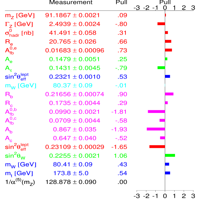
Figure 10: SM electroweak fit as presented in Vancouver by W. Hollik.

All of these corrections are included in the global electroweak fits. The data as well as the pull of the fit is shown in Fig. 10 [28]. All experiments agree with the SM to better than $2\sigma$. The $\chi^{2}/{\rm d.o.f.}=18.4/16$ is excellent [28]. From electroweak precision data there is no hint for any physics beyond the SM. This is unlike the case of the magnetic moment of the proton, which gave a strong indication of a new scale of physics. However, and this is one of the main points of this lecture, supersymmetry can all the same be hiding just around the corner. As we saw for $(g-2)_{\mu}/2$ supersymmetry decouples very rapidly, well before the upper mass bound of $1\,TeV$ imposed by the hierarchy problem. It is therefore no great problem that the electroweak fit is so good.

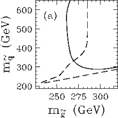
Figure 11: Envelopes of the excluded parameter points at the $95\%$ C.L. shown as the dashed line and the allowed parameter points shown as a solid line in the gluino- and squark-mass plane.

6.2 Radiative Corrections and the MSSM

Within the MSSM, the parameters receive radiative corrections from the superpartners as well, just as in the calculation for $(g_{\mu}-2)/2$. These modify the predictions for other measurements such as that for $(G_{F})_{\mu}$ of Eq.(62). The tree-level result is unmodified, but there are now additional contributions to (i) $\Delta\alpha$ and (ii) $\Delta\rho$ through supersymmetric particles in the vacuum polarization loop. There are also new contributions to $(\Delta r)_{\rm rest}$ as shown for example in Fig. 9b.

In the minimal supergravity model with radiative breaking we have the parameter set

$$\left[\left(\alpha,\,G_{F},\,M_{Z},\,M_{H},m_{top}\right)_{SM};\left(m_{0},\,m_{1/2},\,\tan\beta,\,A_{t},\,sgn(\mu)\right)_{MSSM}\right].$$ (63)

We thus have 9 parameters plus one sign with again more than 25 observables. This is a non-trivial check of the MSSM, a hurdle which technicolour theories for example have great difficulty in passing. The philosophy of the authors in [28] is to let the supersymmetry parameters float freely and thus obtain a preferred value from an optimal fit. The resulting global fit to the data gives a $\chi^{2}/d.o.f=17.3/13$ [28], which is slightly worse than in the SM case but still an excellent fit. We call the resulting value $\chi^{2}_{min}$. As we showed in the case of the anomalous magnetic moment of the muon, the supersymmetric contributions decouple very quickly. It is thus no great surprise, that the data can be fit with heavy supersymmetric masses.

A different philosophy is taken by J. Erler and D. Pierce [29], which is the same philosophy we used above when discussing the supersymmetric contributions to $(g_{\mu}-2)/2$. If we lower the supersymmetric masses the supersymmetric corrections become larger. This is clear in our result for $((g_{\mu}-2)/2)^{susy}$, Eq.(53). Since the SM fit is so good this implies that the overall $\chi^{2}$-fit becomes worse as we lower the masses. In practice the authors scan the MSSM parameter space. At each point in the scan, the constraints from electroweak symmetry breaking, Yukawa perturbativity and direct searches are applied. Points failing these checks are disregarded. For the remaining points, the $\chi^{2}$ is computed. If $\Delta\chi^{2}=\chi^{2}-\chi^{2}_{min}>3.84$, this point is excluded at 95% C.L.. The remaining points are allowed. In Fig. 11 we show the envelopes of the allowed and excluded points in the squark gluino mass-plane. We can read off a lower-bound on the gluino mass of $260\,GeV$ and of the squark mass of $285\,GeV$. The lower bound on the left-handed scalar muon is $105\,GeV$. A full set of bounds is given in a Table in Ref.[29].

7 Supersymmetry Breaking

There is at present no satisfactory model of supersymmetry breaking. Here I only want to discuss the effect of spontaneously breaking global supersymmetry on the super trace formula (10). We shall follow the discussion in Ref.[2]. We thus focus on the bi-linear couplings of all fields to scalar fields.

Figure 12: Supersymmetric couplings contributing to the mass terms for (a) the gauge bosons, (b) chiral fermions, and (c) scalar fermions.

• Vector Masses: The vector bosons can obtain masses from the kinetic term for the scalar fields

  $$({\cal D}_{\mu}\phi)^{\dagger}({\cal D}^{\mu}\phi),$$ (64)

  where ${\cal D}_{\mu}=\partial_{\mu}+igT_{a}A^{a}_{\mu}$, is the covariant derivative, $T_{a}$ is the group generator and $A^{a}_{\mu}$ is the gauge field. The corresponding Feynman diagram is shown in Fig. 12a. The coupling is given by $g^{2}(T_{a}T_{b})_{ij}A^{a}_{\mu}A^{b}_{\nu}\phi^{*}_{i}\phi_{j}$. To obtain the trace of the mass term we must calculate $Tr(T_{a}T_{b})_{ij}=C_{2}(R_{\phi})\delta_{ij}$, where $C_{2}(R_{\phi})$ is the Casimir of the representation of $\phi$ in the gauge group. We thus obtain

  $$Tr{\cal M}_{V}^{2}=g^{2}C_{2}(R_{\phi})\phi^{*}_{i}\phi_{j}.$$ (65)

• Scalar and Chiral Fermion Masses: The Yukawa interaction and the quartic scalar interaction are shown in Fig. 12b and c, respectively. They come from the same superpotential term and are thus related. For the superpotential term $W_{1}=LH_{1}E^{c}$ which includes the term giving mass to the electron, we extract the component interactions via the function ${\overline{W}}_{1}=W_{1}(\phi)=\phi_{L}\phi_{H_{1}}\phi_{E^{c}}$ which is a function of the scalar fields, only. The Yukawa coupling is then given by

  $$\frac{\partial^{2}{\overline{W}}_{1}}{\partial\phi_{L}\partial\phi_{E^{c}}}=\phi_{H_{1}},\quad{\rm where}\quad m_{e}\propto<\phi_{H_{1}}>.$$ (66)

  The quartic scalar coupling is simply twice the Yukawa coupling.

• Fermion Masses: From the previous discussion we obtain for the chiral fermions

  $$m_{ij}=\left|\frac{\partial^{2}{\overline{W}}}{\partial\phi_{i}\partial\phi_{j}}\right|.$$ (67)

  In the SM the gauge bosons can interact with two fermions, e.g. ${\overline{\psi}}_{e}\gamma_{\mu}T^{a}\psi_{e}A^{\mu}_{a}$. In supersymmetry there is a corresponding coupling between the superpartner of the gauge boson (the gauginos, $\lambda_{\tilde{A}}^{a}$), the SM fermion, $\psi_{f}$, and the scalar fermion superpartner, $\phi_{\tilde{f}}$, namely $g{\overline{\psi}}_{e}P_{L}T_{a}\lambda_{A}^{a}\phi_{e}$. This gives a mixing between the gauginos and the chiral fermions. The coupling is proportional to $g(T^{a})_{i}\phi_{i}$. In the basis $(\psi,\lambda)$ the fermion mass matrix then has the form

  $${\cal M}_{F}=\left(\begin{array}[]{cc}a&b\\ b&0\end{array}\right),\quad\Longrightarrow\quad{\cal M}_{F}^{2}=\left(\begin{array}[]{cc}a^{2}+b^{2}&ab\\ ab&0\end{array}\right),$$ (68)

  where $a=\left|\frac{\partial^{2}{\overline{W}}}{\partial\phi_{i}\partial\phi_{j}}\right|$ and $b=gT^{a}_{i}\phi_{i}$. For the trace we then obtain

  $$Tr{\cal M}_{F}^{2}=\left|\frac{\partial^{2}{\overline{W}}}{\partial\phi_{i}\partial\phi_{j}}\right|+2g^{2}C_{2}(R_{\phi})\phi_{i}^{*}\phi_{j},$$ (69)

• Scalar Masses: For the scalar masses we obtain

  $$Tr{\cal M}_{S}^{2}=2\left|\frac{\partial^{2}{\overline{W}}}{\partial\phi_{i}\partial\phi_{j}}\right|+g^{2}C_{2}(R_{\phi})\phi_{i}^{*}\phi_{j}.$$ (70)

  The first term is obtained from the superpotential as discussed above. The second term is obtained from the so-called $D$-term, which also gives the quartic interactions in the Higgs potential.

Next we combine all these terms into the supertrace formula

$$STr{\cal M}^{2} = \sum_{i=s}(-1)^{2S_{i}}(2S_{i}+1)Tr{\cal M}_{J_{i}}^{2}$$ (71)

$$= 3Tr{\cal M}_{V}^{2}+Tr{\cal M}_{S}^{2}-2Tr{\cal M}_{F}^{2}$$

$$= 3\left(g^{2}C_{2}(R_{\phi})\phi^{*}_{i}\phi_{i}\right)+\left(2\left|\frac{\partial^{2}{\overline{W}}}{\partial\phi_{i}\partial\phi_{j}}\right|^{2}+g^{2}C_{2}(R\phi)\phi^{*}_{i}\phi_{i}\right)$$

$$-2\left(\left|\frac{\partial^{2}{\overline{W}}}{\partial\phi_{i}\partial\phi_{j}}\right|^{2}+2g^{2}C_{2}(R_{\phi})\phi^{*}_{i}\phi_{i}\right)$$

$$= 0.$$

We see that all the contributions exactly cancel, independently of the value of the scalar fields $\phi_{i}$. Thus we have $STr{\cal M}^{2}=0$, even if some of the scalar fields receive a nonvanishing vacuum expectation value, $<\phi_{i}>\not=0$. We therefore have in the case of spontaneously broken global supersymmetry that

$$STr{\cal M}^{2}=0.$$ (72)

As discussed in the introduction, this is a catastrophe. For one chiral multiplet we must have one scalar partner with mass less than the fermion mass in Eq.(11).

Of course the spectrum is not restricted to just the electron and its superpartners. In the above derivation we see that the terms deriving from the superpotential (F-terms) cancel separately from those proportional to gauge couplings squared (D-terms). In principle a heavy gaugino could cancel a heavy scalar, letting both be well above their superpartner masses. However, it has proven impossible to construct such models [31].

The solution to the above puzzle is given by radiative corrections. The above formula is only valid at tree-level. It can be violated by higher order terms. We would expect such corrections to be small compared to the SM masses, and the supertrace formula to be violated only weakly. But the required splitting is large, as we saw for the scalar muon mass. The solution is to embed the supersymmetry breaking in a so-called “hidden sector”. This “sector” is a set of fields which do not couple directly to the SM fields. Here supersymmetry is broken spontaneously and at leading order the supertrace vanishes. This breaking is now communicated to the MSSM superfields via radiative corrections. Thus for these fields the radiative corrections offer the only and thus dominant contribution to the breaking mass. They can now have a large splitting from their SM superpartners such as the muon.

At present there are two widely considered models. In one case, supersymmetry breaking is communicated via gauge interactions [30]. In the other case supersymmetry breaking is communicated via gravity [31]. This latter case includes local supersymmetry, where Eq.(72) is modified to

$$STr{\cal M}^{2}=2(N-1)m_{3/2}^{2},$$ (73)

where $N$ is the number of chiral superfields and $m_{3/2}$ is the mass of the gravitino which determines the mass of the SM superpartners. In both cases we have such a hidden sector, where the supersymmetry breaking mechanism hides. It is not clear if this sector will ever be experimentally accessible. So the disguise of supersymmetry, i.e. supersymmetry breaking giving higher masses as for the smuon, is it self out of sight.

8 Summary

Supersymmetry is a well motivated unique extension of the SM. The hierarchy problem indicates that the supersymmetric masses could well be of ${\cal O}(1\,TeV)$. We discussed the simple example of the anomalous magnetic moment of the muon and saw that supersymmetry can indeed be hiding between present experimentally accessible energy scales and ${\cal O}(1\,TeV)$ without disrupting precision measurements, by introducing supersymmetry breaking masses. This is the first disguise of supersymmetry. We then discussed how the breaking mechanism itself is hidden in order to obtain a realistic spectrum.

References

- [1] D. Bailin and A. Love, ‘Supersymmetric Gauge Field Theory and String Theory, IOP Publishing.
- [2] S. Ferrara, L. Girardello, F. Palumbo, Phys. Rev. D20 (1979) 403.
- [3] S. Coleman, J. Mandula, Phys. Rev. 159 (1967) 1251.
- [4] R. Haag, J. T. Lopuszanski, M. Sohnius, Nucl. Phys. B 88 (1975) 257.
- [5] G.G. Ross, ‘Grand Unified Theories’, Benjamin/Cummings 1984.
- [6] E. Gildener, S. Weinberg, Phys. Rev. D 13 (1976) 3333; E. Gildener, Phys. Rev. D 14 (1976) 1667.
- [7] M. Drees, lectures given at Inauguration Conference of the Asia Pacific Center for Theoretical Physics, hep-ph/9611409.
- [8] Y. Fukuda et al., the Super-Kamiokande Collaboration, Phys. Rev. lett. 81 (1998) 1562.
- [9] M.B. Gavela, P. Hernandez, J. Orloff, O. Pene, Mod. Phys. Lett. A9 (1994) 795, hep-ph/9312215; Nucl. Phys. B430 (1994) 382, hep-ph/9406289; P. Huet, E. Sather, Phys. Rev. D51 (1995) 379, hep-ph/9404302; K. Kajantie, M. Laine, K. Rummukainen, M. Shaposhnikov, Nucl. Phys. B493 (1997) 413, hep-lat/9612006.
- [10] For a recent contribution see: M. Carena, M. Quiros, C.E.M. Wagner, Nucl. Phys. B 524 (1998) 3, hep-ph/9710401.
- [11] T. Hambye, K. Riesselmann, Phys. Rev. D55 (1997) 7255, hep-ph/9610272.
- [12] M. Dittmar, H. Dreiner, Phys. Rev. D 55 (1997) 167, hep-ph/9608317; Proceedings of the Ringberg Higgs Workshop, 8-13 Dec 1996, hep-ph/9703401.
- [13] For a review on R-parity violation see H. Dreiner, hep-ph/9707435.
- [14] H. Dreiner, G.G. Ross, Nucl. Phys. B 365 (1991) 597.
- [15] Seminars presented to the LEPC by the ALEPH, DELPHI, L3 and OPAL collaborations on Nov. 12, 1998.
- [16] H. Haber, talk given at SUSY-97, Philadelphia, May 1997, hep-ph/9709450, Nucl. Phys. Proc. Suppl. 62 (1998) 469.
- [17] For a review see L. E. Ibanez, G. G. Ross, in ‘Perspectives on Higgs physics’, Edited by G. Kane, World Scientific, 1993, hep-ph/9204201.
- [18] M. Peskin and D.V. Schroeder, ‘An Introduction to Quantum Field Theory’, Addison-Wesley (1995).
- [19] S. Weinberg, ‘The Quantum Theory of Fields’, Vol. 1, Cambridge Univ. Pr. (1995).
- [20] Particle Data group, Review of Particle Properties, Phys. Rev. D 54 (1996) 720.
- [21] For a recent summary of the SM calculations as well as a new contribution on the anomalous magnetic moment of the muon see for example G. Degrassi, G.F. Giudice, Phys. Rev. D58 (1998) 053007, hep-ph/9803384.
- [22] M. Carena, G.F. Giudice, C.E.M. Wagner, Phys. Lett. B 390 (1997) 234, hep-ph/9610233.
- [23] See page 188 in [18].
- [24] P. Fayet, in Unification of the Fundamental Particle Interactions, eds. S. Ferrara, J. Ellis and P. van Nieuwenhuizen (Plenum Press, New York, 1980) p. 587.
- [25] J. Grifols and A. Mendez, Phys. Rev. D26 (1982) 1809.
- [26] J. Ellis, J. Hagelin and D.V. Nanopoulos, Phys. Lett. B 116 (1982) 283; R. Barbieri and L. Maiani, Phys. Lett. B 117 (1982) 203; T.C. Yuan, R. Arnowitt, and A.H. Chamseddine, Z. Phys. C 26 (1984) 407.
- [27] T. Moroi, Phys. Rev. D 53 (1996) 6565, Erratum-ibid. D 56 (1997) 4424, hep-ph/9512396.
- [28] W. Hollik, Talk given at 29th International Conference on High-Energy Physics, Vancouver, Canada, July 1998, hep-ph/9811313; S. Heinemeyer, W. Hollik, G. Weiglein, hep-ph/9807423.
- [29] J. Erler and D. Pierce, Nucl. Phys. B 526 (1998) 53, hep-ph/9801238.
- [30] For a recent review see G.F. Giudice, and R. Rattazzi, hep-ph/9801271.
- [31] H.P. Nilles, Phys. Rept. 110 (1984) 1.