[

FERMILAB-PUB-99/022-T

UCSD/PTH/99-01

Ab Initio Study of Hybrid ${\rm\overline{\mathbf{b}}\mathbf{gb}}$ Mesons

K.J. Juge,¹ J. Kuti$,^{2}$ and C.J. Morningstar²

¹ Fermi National Accelerator Laboratory, P.O. Box 500, Batavia, IL 60510

²Dept. of Physics, University of California at San Diego, La Jolla, California 92093-0319

(February 12, 1999)

Hybrid ${\rm\overline{b}gb}$ molecules in which the heavy ${\rm\overline{b}b}$ pair is bound together by the excited gluon field g are studied using the Born-Oppenheimer expansion and quenched numerical simulations. The consistency of results from the two approaches reveals a simple and compelling physical picture for heavy hybrid states.

PACS number(s): 11.15.Ha, 12.38.Gc, 12.39.Mk

]

In addition to conventional hadrons, QCD predicts the existence of glueballs and hybrid states which contain excited gluon fields. Hybrid mesons with heavy ${\rm\overline{b}b}$ quark pairs are the most amenable to theoretical treatment. They are also experimentally accessible: early results from the CUSB and CLEO collaborations[1, 2] revealed a complex resonance structure between the $\rm{\overline{B}B}$ threshold and 11.2 GeV in $\rm{e^{+}e^{-}}$ annihiliation, precisely where the lowest hybrid excitations are expected[3].

In this work, we determine the masses of the lowest ${\rm\overline{b}gb}$ states. Heavy hybrid mesons can be studied not only directly by numerical simulation, but also using the Born-Oppenheimer expansion which is our primary guidance for the development of a simple physical picture. The Born-Oppenheimer picture was introduced for the description of heavy hybrid states in Refs. [4, 5] and was applied using hybrid potentials first calculated in lattice QCD in Ref. [6]. In this new study, we work to leading order in the expansion and neglect higher-order terms involving spin, relativistic, and retardation effects. We test the accuracy of the Born-Oppenheimer approach by comparison with high-precision results from simulations.

Our hybrid meson simulations are the first to exploit anisotropic lattices with improved actions; preliminary reports on some of our results have appeared previously[7]. The hybrid meson mass uncertainties with improved anisotropic lattice technology are dramatically smaller than those obtained in recent isotropic lattice studies in the nonrelativistic formulation of lattice QCD (NRQCD) using the Wilson gauge action[8, 9]. We report here our final analysis on four distinct hybrid ${\rm\overline{b}gb}$ states. Although the effects of dynamical sea quarks are not included in our quenched simulations, we will comment on their impact on the hybrid spectrum. The mass of the lowest hybrid ${\rm\overline{c}gc}$ state was determined recently[10] without NRQCD expansion for the slowly moving heavy quark and agrees with our Born-Oppenheimer results[3] (see caption of Fig. 1).

The hybrid meson can be treated analogous to a diatomic molecule: the slow heavy quarks correspond to the nuclei and the fast gluon field corresponds to the electrons[4]. First, one treats the quark $\mathrm{Q}$ and antiquark $\overline{\mathrm{Q}}$ as spatially-fixed color sources and determines the energy levels of the excited gluon field as a function of the $\overline{\mathrm{Q}}\mathrm{Q}$ separation $\mathrm{r}$; each of these excited energy levels defines an adiabatic potential $V_{\overline{\mathrm{Q}}\mathrm{gQ}}(\mathrm{r})$. The quark motion is then restored by solving the Schrödinger equation in each of these potentials. Conventional quarkonia are based on the lowest-lying static potential; hybrid quarkonium states emerge from the excited potentials. Once the static potentials have been determined (via lattice simulations), it is a simple matter to determine the complete spectrum of conventional and hybrid quarkonium states in the leading Born-Oppenheimer (LBO) approximation. This is a distinct advantage over meson simulations which yield only the very lowest-lying states, often with large statistical uncertainties. In addition, the LBO wave functions yield valuable information concerning the structures and sizes of these states which should greatly facilitate phenomenological applications.

The energy spectrum of the excited gluon field in the presence of a static quark-antiquark pair has been determined in previous lattice studies[7]. The three lowest-lying levels are shown in Fig. 1. These levels correspond to energy eigenstates of the excited gluon field characterized by the magnitude $\Lambda$ of the projection of the total angular momentum ${\bf J}_{\mathrm{g}}$ of the gluon field onto the molecular axis, and by $\eta=\pm 1$, the symmetry quantum number under the combined operations of charge conjugation and spatial inversion about the midpoint between the quark and antiquark of the ${\rm\overline{Q}gQ}$ system. Following notation from molecular spectroscopy, states with $\Lambda=0,1,2,\dots$ are typically denoted by the capital Greek letters $\Sigma,\Pi,\Delta,\dots$, respectively. States which are even (odd) under the above-mentioned parity–charge-conjugation operation are denoted by the subscripts $\mathrm{g}$ ($\mathrm{u}$). There is an additional label for the $\Sigma$ states; $\Sigma$ states which are even (odd) under a reflection in a plane containing the molecular axis are denoted by a superscript $+$ $(-)$. In Ref. [7], the potentials are calculated in terms of the hadronic scale parameter ${\rm r_{0}}$ [11]; the curves in Fig. 1 assume ${\rm r_{0}^{-1}=450}$ MeV (see below). Note that as $\mathrm{r}$ becomes small (below 0.1 fm), the gaps between the excited levels and the $\Sigma_{\mathrm{g}}^{+}$ ground state will eventually exceed the mass of the lightest glueball. When this happens, the excited levels will become unstable against glueball decay.

Given these static potentials, the LBO spectrum is easily obtained by solving the radial Schrödinger equation with a centrifugal factor ${\rm\langle{\bf L}_{\overline{Q}Q}^{2}\rangle=L(L+1)-2\Lambda^{2}+\langle{\bf J}_{g}^{2}\rangle}$, where ${\rm{\bf L}_{\overline{Q}Q}}$ is the orbital angular momentum of the quark–antiquark pair. For the $\Sigma_{\mathrm{g}}^{+}$ potential, $\langle{\bf J}_{\mathrm{g}}^{2}\rangle=0$. For the $\Pi_{\mathrm{u}}$ and $\Sigma_{\mathrm{u}}^{-}$ levels, we attribute the lowest nonvanishing value $\langle{\bf J}_{\mathrm{g}}^{2}\rangle=2$ to the excited gluon field. Let ${\bf S}$ be the sum of the spins of the quark and antiquark, then the total angular momentum of a meson is given by ${\bf J}={\bf L}+{\bf S}$. In the LBO approximation, the eigenvalues ${\rm L(L+1)}$ and ${\rm S(S+1)}$ of ${\bf L}^{2}$ and ${\bf S}^{2}$ are good quantum numbers. The parity ${\rm P}$ and charge conjugation ${\rm C}$ of each meson is given in terms of ${\rm L}$ and ${\rm S}$ by ${\rm P=\epsilon\ (-1)^{L+\Lambda+1}}$ and ${\rm C=\epsilon\ \eta\ (-1)^{L+\Lambda+S}}$, where ${\rm L\geq\Lambda}$ and $\epsilon=1$ for $\Sigma^{+}$, $\epsilon=-1$ for $\Sigma^{-}$, and $\epsilon=\pm 1$ for $\Lambda>0$. Note that for each static potential, the LBO energies depend only on ${\rm L}$ and the radial quantum number ${\rm n}$.

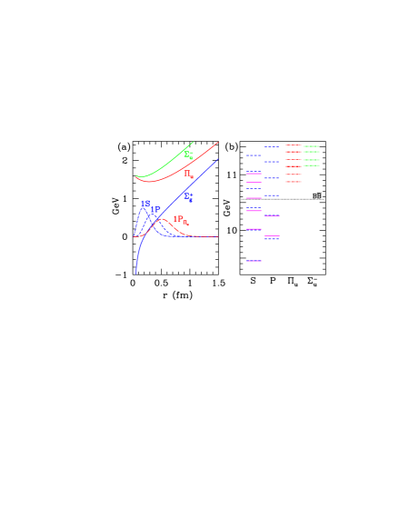
FIG. 1.: (a) Static potentials and radial probability densities against quark-antiquark separation ${\rm r}$ for ${\rm r_{0}^{-1}=450}$ MeV. The $\Sigma_{\mathrm{g}}^{+}$ potential becomes the familiar running Coulomb law as ${\rm r}$ becomes very small. (b) Spin-averaged ${\rm\bar{b}b}$ spectrum in the LBO approximation (light quarks neglected). Solid lines indicate experimental measurements. Short dashed lines indicate the $\mathrm{S}$ and $\mathrm{P}$ state masses obtained from the Schrödinger equation with the $\Sigma_{\mathrm{g}}^{+}$ potential for ${\rm M_{b}=4.58}$ GeV. Dashed-dotted lines indicate the hybrid quarkonium states obtained from the $\Pi_{\mathrm{u}}$ ${\rm(L=1,2,3)}$ and $\Sigma_{\mathrm{u}}^{-}$ ${\rm(L=0,1,2)}$ potentials. Repeating the same analysis in the ${\rm\overline{c}gc}$ system, we find the lowest $\Pi_{\mathrm{u}}$ hybrid ${\rm 1.19~{}GeV}$ above the spin averaged ground state.

Results for the LBO spectrum of conventional ${\rm\overline{b}b}$ and hybrid ${\rm\overline{b}gb}$ states are shown in Fig. 1. The heavy quark mass ${\rm M_{b}}$ is tuned to reproduce the experimentally-known ${\rm\Upsilon(1S)}$ mass: ${\rm M_{\Upsilon}=2M_{b}+E_{0}}$, where ${\rm E_{0}}$ is the energy of the lowest-lying state in the $\Sigma_{\mathrm{g}}^{+}$ potential. Level splittings are insensitive to small changes in the heavy quark mass. For example, a $5\%$ change in ${\rm M_{b}}$ results in changes to the splittings (with respect to the $1S$ state) ranging from $0.1-0.8\%$.

Below the $\overline{B}B$ threshold, the LBO results are in very good agreement with the spin-averaged experimental measurements of bottomonium states. Above the threshold, agreement with experiment is lost, suggesting significant corrections from higher order effects and possible mixings between the states from different adiabatic potentials. The mass of the lowest-lying hybrid (from the $\Pi_{\mathrm{u}}$ potential) is about 10.9 GeV. Hybrid mesons from all other hybrid potentials are significantly higher lying. The radial probability densities for the conventional ${\rm 1S}$ and ${\rm 1P}$ states are compared with that of the lowest-lying $\Pi_{\mathrm{u}}$ hybrid state in Fig. 1. Note that the size of the hybrid state is large in comparison with the ${\rm 1S}$ and ${\rm 1P}$ states. For all of the hybrid states studied here, the wave functions are strongly suppressed near the origin so that the hybrid masses cannot be affected noticeably by the small-${\rm r}$ instability of the excited-state potentials from ${\rm\overline{b}gb\rightarrow\overline{b}b+glueball}$ decay.

The applicability of the Born-Oppenheimer approximation relies on the smallness of retardation effects. The difference between the leading Born-Oppenheimer Hamiltonian and the lowest order NRQCD Hamiltonian is the ${\rm\vec{p}\cdot\vec{A}}$ coupling between the quark color charge in motion and the gluon field. This retardation effect, which is not included in the LBO spectrum, can be tested by comparing the LBO mass splittings with those determined from meson simulations in NRQCD.

In order to obtain the masses of the first few excited hybrid states in a given symmetry channel, we obtained Monte Carlo estimates for a matrix of hybrid meson correlation functions ${\rm C_{ij}(t)=\langle 0|M_{i}(t)M_{j}^{\dagger}(0)|0\rangle}$ at two different lattice spacings. Because the masses of the hybrid mesons are expected to be rather high and the statistical fluctuations large, it is crucial to use anisotropic lattices in which the temporal lattice spacing ${\rm a_{t}}$ is much smaller than the spatial lattice spacing ${\rm a_{s}}$. Such lattices have already been used to dramatically improve our knowledge of the Yang-Mills glueball spectrum[12]. In our simulations, the gluons are described by the improved gauge-field action of Ref.[12]. The couplings $\beta$, input aspect ratios $\xi$, and lattice sizes for each simulation are listed in Table I. Following Ref. [12], we set the mean temporal link ${\rm u_{t}=1}$ and obtain the mean spatial link ${\rm u_{s}}$ from the spatial plaquette. The values for ${\rm r_{0}}$ in terms of ${\rm a_{s}}$ corresponding to each simulation were determined in separate simulations. Further details concerning the calculation of ${\rm r_{0}/a_{s}}$ are given in Ref. [12]. Note that we set the aspect ratio using ${\rm a_{s}/a_{t}=\xi}$ in all of our calculations. By extracting the static-quark potential from Wilson loops in various orientations on the lattice[13], we have verified that radiative corrections to the anisotropy ${\rm a_{s}/a_{t}}$ are small. The heavy quarks are treated within the NRQCD framework [14], modified for an anisotropic lattice. The NRQCD action includes only a covariant temporal derivative and the leading kinetic energy operator (with two other operators to remove ${\rm O(a_{t})}$ and ${\rm O(a_{s}^{2})}$ errors); relativistic corrections depending on spin, the chromoelectric ${\bf E}$ and chromomagnetic ${\bf B}$ fields, and higher derivatives are not included.

TABLE I.: Simulation parameters and results. The second errors listed in the results in the bottom six rows are due to uncertainties in setting the heavy quark mass.

$(\beta,\xi)$	$(3.0,3)$	$(2.6,3)$
${\rm u_{s}^{4}}$	$0.500$	0.451
lattice	$15^{3}\!\times\!45$	$10^{3}\!\times\!30$
$\#$ configs, sources	201, 16080	355, 17040
${\rm r_{0}/a_{s}}$	4.130(24)	2.493(9)
${\rm(\zeta,n_{\zeta})}$	$(0.25,15)$	$(0.15,10)$
${\rm a_{s}M_{0}}$	$2.56$	$3.90$
${\rm a_{s}M^{S}_{\rm kin}}$	$5.03(2)$	$8.21(1)$
${\rm r_{0}\;\delta(1P-1S)}$	$0.959(8)(3)$	$0.998(6)(3)$
${\rm r_{0}\;\delta(2S-1S)}$	$1.303(11)(10)$	$1.252(8)(10)$
${\rm r_{0}\;\delta(H_{1}-1S)}$	$3.287(53)(20)$	$3.338(54)(20)$
${\rm r_{0}\;\delta(H_{2}-1S)}$	$3.37(13)(1)$	$3.443(47)(10)$
${\rm r_{0}\;\delta(H_{3}-1S)}$	$4.018(55)(12)$	$4.034(76)(12)$
${\rm r_{0}\;\delta(H_{1}^{\prime}-1S)}$	$4.204(67)(21)$	$4.229(62)(21)$

Our meson operators ${\rm M_{i}(t)}$ are constructed on a given time-slice as follows. First, the spatial link variables are smeared using the algorithm of Ref. [15] in which every spatial link ${\rm U_{j}(x)}$ on the lattice is replaced by itself plus $\zeta$ times the sum of its four neighboring spatial staples, projected back into SU(3); this procedure is iterated ${\rm n_{\zeta}}$ times, and we denote the final smeared link variables by ${\rm\tilde{U}_{j}(x)}$. Next, let ${\rm\psi(x)}$ and ${\rm\chi(x)}$ denote the Pauli spinor fields which annihilate a heavy quark and antiquark, respectively. Note that the antiquark field is defined such that ${\rm C\psi(x)C^{\dagger}=i\sigma_{y}\chi^{\ast}(x)}$, where ${\rm C}$ is the charge conjugation operator. We define a smeared quark field by $\tilde{\psi}(\mathrm{x})\equiv\left(1+\varrho\ a_{\mathrm{s}}^{2}\tilde{\Delta}^{(2)}\right)^{n_{\varrho}}\psi(\mathrm{x}),$ (and similarly for the antiquark field) where $\varrho$ and ${\rm n_{\varrho}}$ are tunable parameters (we used $\varrho=0.12,0.14$ and ${\rm n_{\varrho}=2-7}$) and the covariant derivative operators are defined in terms of the smeared link variables ${\rm\tilde{U}_{j}(x)}$. These field operators, in addition to the chromomagnetic field, are then used to construct our meson operators, which are listed in Table II. The standard clover-leaf definition of the chromomagnetic field $\tilde{\bf B}$ is used, defined also in terms of the smeared link variables. Note that four operators are used in each of the $0^{-+}$ and $1^{--}$ sectors. Because our NRQCD action includes no spin interactions, we use only spin-singlet operators. We can easily couple these operators to the quark-antiquark spin to obtain various spin-triplet operators, and the masses of such states will be degenerate with those from the spin-singlet operators.

TABLE II.: The meson spin-singlet operators used in each total angular momentum ${\rm J}$, parity ${\rm P}$, and charge conjugation ${\rm C}$ channel. Note that ${\rm p=0,1,2,}$ and $3$ were used to produce four distinct operators in the $0^{-+}$ and $1^{--}$ sectors. In the third column are listed the spin-triplet states which can be formed from the operators in the last column; the states in each row are degenerate for the NRQCD action used here.

$J^{PC}$		Degeneracies	Operator
$0^{-+}$	${\rm S}$ wave	$1^{--}$	$\tilde{\chi}^{\dagger}\ \left[\tilde{\Delta}^{(2)}\right]^{p}\ \tilde{\psi}$
$1^{+-}$	${\rm P}$ wave	$0^{++},1^{++},2^{++}$	$\tilde{\chi}^{\dagger}\ \tilde{\mbox{\boldmath{$\Delta$}}}\ \tilde{\psi}$
$1^{--}$	${\rm H_{1}}$ hybrid	$0^{-+},1^{-+},2^{-+}$	$\tilde{\chi}^{\dagger}\ \tilde{\bf B}\left[\tilde{\Delta}^{(2)}\right]^{p}\ \tilde{\psi}$
$1^{++}$	${\rm H_{2}}$ hybrid	$0^{+-},1^{+-},2^{+-}$	$\tilde{\chi}^{\dagger}\ \tilde{\bf B}\!\times\!\tilde{\mbox{\boldmath{$\Delta$}}}\ \tilde{\psi}$
$0^{++}$	${\rm H_{3}}$ hybrid	$1^{+-}$	$\tilde{\chi}^{\dagger}\ \tilde{\bf B}\!\cdot\!\tilde{\mbox{\boldmath{$\Delta$}}}\ \tilde{\psi}$

In each simulation, the bare quark mass ${\rm a_{s}M_{0}}$ is set by matching the ratio ${\rm R=M_{\rm kin}^{S}/\delta(1P-1S)}$, where ${\rm M_{\rm kin}^{S}}$ is the so-called kinetic mass of the ${\rm 1S}$ state and ${\rm\delta(1P-1S)}$ is the energy separation between the ${\rm 1S}$ and ${\rm 1P}$ states, to its observed value $21.01(6)$. The kinetic mass ${\rm M_{kin}^{S}}$ is determined by measuring the energy of the ${\rm 1S}$ state for momenta ${\rm\vec{p}=(0,0,0)}$, ${\rm 2\pi(1,0,0)/L}$, and ${\rm 2\pi(1,1,0)/L}$, where ${\rm L}$ is the spatial extent of the periodic lattice. These three energies are then fit using ${\rm E_{0}+\vec{p}^{2}/(2M_{\rm kin}^{S})}$ to extract ${\rm M_{\rm kin}^{S}}$. Several low statistics runs using a range of quark masses were done in order to tune the quark mass. From the results of these runs, we estimate that the uncertainty in tuning the quark mass is about $5\%$.

The simulation results are listed in Table I. The masses ${\rm m_{i}}$ in the $1^{+-}$, $1^{++}$, and $0^{++}$ channels are extracted by fitting the single correlators ${\rm C_{i}(t)}$ to their expected asymptotic form ${\rm C_{i}(t)\rightarrow Z_{i}\exp(-m_{i}t)}$ for sufficiently large ${\rm t}$. In each of the $0^{-+}$ and $1^{--}$ channels, we obtain a $4\times 4$ correlation matrix. The variational method is then applied to reduce the $4\times 4$ matrix down to an optimized $2\times 2$ correlation matrix ${\rm C^{opt}_{ij}(t)}$. For sufficiently large ${\rm t}$, we fit all elements of this matrix using ${\rm\sum_{p=0}^{1}Z_{ip}Z_{jp}\exp(-m_{p}t)}$ to extract the two lowest-lying masses. In this way, we obtain an estimate of the ${\rm 2S}$ mass, as well as the first excited hybrid state ${\rm H_{1}^{\prime}}$. The effective masses corresponding to several of the correlation functions obtained in the $\beta=3.0$, $\xi=3$ simulation are shown in Fig. 2.

FIG. 2.: Effective masses ${\rm m_{\rm eff}(t)=-\ln[C(t+a_{t})/C(t)]}$ for two of the hybrids from the $(\beta,\xi)=(3.0,3)$ simulation.

The simulation results for the level splittings (in terms of ${\rm r_{0}}$ and with respect to the ${\rm 1S}$ state) are shown in Fig. 3 against the lattice spacing. Small finite–${\rm a_{s}}$ errors are evident in the ${\rm 1P}$ and ${\rm 2S}$ splittings from the coarse lattice simulation; none of the four hybrid splittings show any significant discretization errors. The simulation results compare remarkably well with the LBO predictions, shown as horizontal lines in Fig. 3. In the LBO approximation, the ${\rm H_{1}}$ and ${\rm H_{2}}$ mesons correspond to degenerate ${\rm 1P_{\Pi_{u}}}$ states of opposite $\epsilon$, the ${\rm H_{3}}$ hybrid corresponds to a ${\rm 1S_{\Sigma_{u}^{-}}}$ state, and the ${\rm H_{1}^{\prime}}$ corresponds to a ${\rm 2P_{\Pi_{u}}}$ level; furthermore, the ${\rm H_{3}}$ and ${\rm H_{1}^{\prime}}$ hybrids are predicted to be nearly degenerate, with the ${\rm H_{1}^{\prime}}$ lying slightly lower. The simulation results share these same qualitative features, except that the ${\rm H_{1}^{\prime}}$ lies slightly higher than the ${\rm H_{3}}$. The LBO approximation reproduces all of the level splittings to within $10\%$. In Fig. 3, we also show results[16] for the ${\rm 1P}$ and ${\rm 2S}$ splittings for an NRQCD action including higher order relativistic and spin interactions; the effects of such terms are seen to be very small. Note that spin-dependent mass splittings are difficult to estimate in hybrid states since the excited gluon field extends on the scale of the confinement radius with a nonperturbative wavefunction when its color magnetic moment interacts with the heavy-quark spins.

To convert our mass splittings into physical units, we must specify the value of ${\rm r_{0}}$. Using the observed value for the ${\rm 1P-1S}$ splitting, we find that ${\rm r_{0}^{-1}=467(4)}$ MeV; using the ${\rm 2S-1S}$ splitting, we obtain ${\rm r_{0}^{-1}=435(5)}$ MeV. This discrepancy is caused by our neglect of light quark effects[17]. Taking ${\rm r_{0}^{-1}=450(15)}$ MeV, our lowest-lying hybrid state lies $1.49(2)(5)$ GeV (the second error is the uncertainty from ${\rm r_{0}}$) above the ${\rm 1S}$ state.

Hybrid and conventional states substantially extending over 1 fm in diameter are vulnerable to light-quark vacuum polarization loops which will dramatically change the static potentials through configuration mixing with ${\rm\overline{B}B}$ mesons; instead of rising indefinitely with ${\mathrm{r}}$, these potentials will eventually level off since the heavy ${\rm\overline{\mathrm{Q}}\mathrm{gQ}}$ state can undergo fission into two separate ${\rm\overline{Q}q}$ color singlets, where ${\rm q}$ is a light quark. We expect that the plethora of hybrid and conventional states above 11 GeV obtained from the quenched potentials will not survive this splitting mechanism as observable resonances. For quark-antiquark separations below 1.2 fm or so, there is evidence from recent studies[18, 3] that light-quark vacuum polarization effects do not appreciably alter the $\Sigma_{\mathrm{g}}^{+}$ and $\Pi_{\mathrm{u}}$ inter-quark potentials (for light-quark masses such that ${\rm m_{\pi}\sim m_{\rho}/2}$). Since such distances are the most relevant for forming the lowest-lying bound states, the survival of the lightest ${\rm\overline{b}gb}$ hybrids as well-defined resonances above the ${\rm\overline{B}B}$ threshold remains conceivable.

During the preparation of this work we learned about new results [19] which have considerable overlap with our NRQCD simulations.

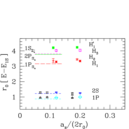
FIG. 3.: Simulation results for the level splittings (in terms of ${\rm r_{0}}$ and with respect to the $1S$ state) against the lattice spacing ${\rm a_{s}}$. Results from Ref. [16] using an NRQCD action with higher-order corrections are shown as $\Box$ and $\bigtriangleup$; all other symbols indicate results from this work. Some points have been shifted horizontally to prevent overlaps. The horizontal lines show the LBO predictions.

This work was supported by the U.S. DOE, Grant No. DE-FG03-97ER40546.

REFERENCES

- [1] D. Lovelock et al., Phys. Rev. Lett. 54, 377 (1985).
- [2] D. Besson et al., Phys. Rev. Lett. 54, 381 (1985).
- [3] J. Kuti, Proceedings of the XVI International Symposium on Lattice Field Theory, Nucl. Phys. B(Proc. Suppl.) in press; hep-lat/9811021.
- [4] P. Hasenfratz, R. Horgan, J. Kuti, J. Richard, Phys. Lett. B95, 299 (1980).
- [5] D. Horn and J. Mandula, Phys. Rev. D17, 898 (1978).
- [6] S. Perantonis and C. Michael, Nucl. Phys., B347 (1990) 854.
- [7] K.J. Juge, J. Kuti, and C. Morningstar, Nucl. Phys. B(Proc. Suppl.) 63 326, (1998); and unpublished (hep-lat/9809098).
- [8] S. Collins, C. Davies, G. Bali, Nucl. Phys. B(Proc. Suppl.)63, 335 (1998).
- [9] T. Manke et al., Phys. Rev. D57, 3829 (1998).
- [10] C. Bernard et al., Phys. Rev. D56, 7039 (1997).
- [11] R. Sommer, Nucl. Phys. B411, 839 (1994).
- [12] C. Morningstar and M. Peardon, Phys. Rev. D56, 4043 (1997); and to appear (hep-lat/9901004).
- [13] C. Morningstar, Nucl. Phys. B(Proc. Suppl.)53, 914 (1997).
- [14] G. P. Lepage, et al., Phys. Rev. D46, 4052 (1992).
- [15] M. Albanese et al., Phys. Lett. B192, 163 (1987).
- [16] C. Davies et al., Phys. Rev. D58, 054505 (1998).
- [17] C. Davies et al., Nucl. Phys. B(Proc. Suppl.)47, 409 (1996); A. Spitz et al., Nucl. Phys. B(Proc. Suppl.)63, 317 (1998).
- [18] G. Bali, private communication, unpublished.
- [19] T. Manke et al., unpublished (hep-lat/9812017).