Triple gauge boson couplings between $\mathrm{Z}^{0}$, $\gamma$ and the W boson are determined by exploiting their impact on radiative corrections to fermion-pair production in e⁺e^- interactions at centre-of-mass energies near the $\mathrm{Z}^{0}$-pole. Recent values of observables in the electroweak part of the Standard model are used to determine the four parameters $\epsilon_{1}$, $\epsilon_{2}$, $\epsilon_{3}$ and $\epsilon_{b}$. In a second step the results on the four $\epsilon$ parameters are used to determine the couplings $\Delta g^{1}_{Z}$ and $\Delta\kappa_{\gamma}$. For a wide range of scales, these indirect coupling measurements are more precise than recent direct measurements at LEP 2 and at the TEVATRON. The Standard model predictions agree well with these measurements.

1 Introduction

One of the most prominent goals of the LEP 2 program performed at the Large Electron Positron Collider (LEP) is the precise measurement of the couplings between the neutral electroweak bosons $\mathrm{Z}^{0}$, $\gamma$ and the charged boson $\mathrm{W}^{\pm}$ [1]. Analogous measurements were performed at the TEVATRON measuring mainly the coupling between the photon and the $\mathrm{W}^{\pm}$. These two measurements were the first ones which were able to prove the non-Abelian character of the electroweak part of the Standard model [2]. Even more precise determinations will be possible at future hadron or electron-positron-collider.

However, before the LEP 2 program with centre-of-mass energies above the W-pair production threshold of about 161 GeV, LEP was running at energies around the $\mathrm{Z}^{0}$-pole at 91 GeV allowing to perform very precise measurements of fermion pair production properties. The experiments at LEP-1 and also at SLAC measure radiative corrections to the $\mathrm{Z}^{0}$ff vertex. These radiative corrections involve contributions with WWV (V=$\mathrm{Z}^{0}$, $\gamma$) vertices as shown in figure 1 a) and b) and WWV-independent contributions (figure 1 c,d). Therefore precise measurements of fermion-pair production allow the determination of the WWV coupling constants. This was noted already in the beginning of the LEP era [3, 4].

The phenomenological effective Lagrangian of the WWZ and WW$\gamma$ vertices, respecting only Lorentz-invariance, contains 14 triple gauge coupling constants (TGCs) as free parameters. All of these can be accommodated in the Standard Model requesting SU(2)$\times$U(1) gauge invariance, if one considers higher dimensional SU(2)$\times$U(1) gauge invariant operators. The neglect of higher dimensional operators leads automatically to relations between TGCs. The model which is discussed in the following neglects operators having a higher dimension than six. Loop corrections in this model lead to a logarithmic divergence of low energy observables [3]. However it was shown that three dimension-six operators, that induce non-standard TGCs do not have this property[4]. Assuming the existence of a light Higgs boson, created by the Higgs-doublet field $\Phi$, one can apply a linear realization of the SU(2)$\times$U(1) symmetry. Then one obtains in addition to the SM Lagrangian the following three terms [4] :

$$\Delta{\cal L} =\imath g^{\prime}\frac{\Delta\kappa_{\gamma}-\cos^{2}\theta_{W}\Delta g^{1}_{Z}}{m^{2}_{W}}(D_{\mu}\Phi)^{\dagger}B^{\mu\nu}(D_{\nu}\Phi)+\imath g\frac{\cos^{2}\theta_{W}\Delta g^{1}_{Z}}{m^{2}_{W}}(D_{\mu}\Phi)^{\dagger}\vec{\tau}\cdot\vec{\hat{W}}^{\mu\nu}(D_{\nu}\Phi)$$

$$+\imath g\frac{\lambda_{\gamma}}{6m^{2}_{W}}\vec{\hat{W}}B^{\mu}_{\nu}\cdot(\vec{\hat{W}}B^{\nu}_{\rho}\times\vec{\hat{W}}B^{\rho}_{\mu}).$$ (1)

In this model the TGC-relations are :

$$\Delta\kappa_{\gamma} =\frac{\cos^{2}\theta_{W}}{\sin^{2}\theta_{W}}(\Delta\kappa_{Z}-\Delta g^{1}_{Z}),$$ (2)

$$\lambda_{\gamma} =\lambda_{Z}.$$ (3)

The remaining nine coupling constants are zero. The SM predicts that all 14 parameters are zero. The TGCs $\Delta\kappa_{V}$ and $\Delta g^{1}_{V}$ parametrise the difference of $g^{1}_{V}$ and $\kappa_{V}$ to its SM expectation of unity :

$$\Delta\kappa_{V}=\kappa_{V}-1$$ (4)

$$\Delta g^{1}_{V}=g^{1}_{V}-1$$ (5)

In almost all models the electromagnetic gauge invariance is taken for granted, such that $\Delta g^{1}_{\gamma}$, the divergence of the W-charge from the unit charge, is always zero. The parameter $\lambda_{\gamma}$ is also set to zero in our analysis, since we are not aware of any computation of the dependence of $\epsilon_{1}$, $\epsilon_{2}$ and $\epsilon_{3}$ on $\lambda_{\gamma}$.

2 Analysis and Results

The preliminary measurements of electroweak parameters performed at LEP 1, SLAC and TEVATRON are listed in table 1. The SM predictions agree well with these measurements [5]. The analysis of this data set proceeds via two steps. In the first step, the $\epsilon$ parameters $\epsilon_{1}$, $\epsilon_{2}$, $\epsilon_{3}$ and $\epsilon_{b}$ [6]:

$$\epsilon_{1} =\Delta\rho$$ (6)

$$\epsilon_{2} =\cos^{2}\theta_{W}^{0}\Delta\rho+\frac{\sin^{2}\theta_{W}^{0}\Delta r_{W}}{\cos^{2}\theta_{W}^{0}-\sin^{2}\theta_{W}^{0}}-2\sin^{2}\theta_{W}^{0}\Delta k^{\prime}$$ (7)

$$\epsilon_{3} =\cos^{2}\theta_{W}^{0}\Delta\rho+(\cos^{2}\theta_{W}^{0}-\sin^{2}\theta_{W}^{0})\Delta k^{\prime}$$ (8)

$$\epsilon_{b} =\frac{g_{A}^{b}}{g_{A}^{l}}-1\quad\hbox{and}\quad\epsilon_{b}=\frac{g_{V}^{b}}{g_{A}^{l}}-\left(1-\frac{4}{3}(1+\Delta k^{\prime})\sin^{2}\theta_{W}^{0}\right)$$ (9)

where:

$$\sin^{2}\theta_{W}^{0} = \frac{\pi\alpha(m^{2}_{Z})}{\sqrt{2}G_{F}m^{2}_{Z}}$$ (10)

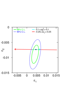
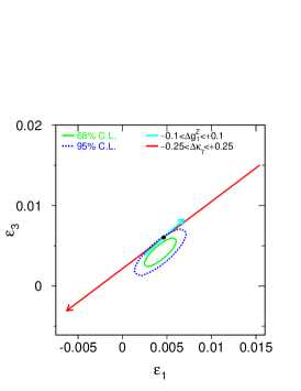
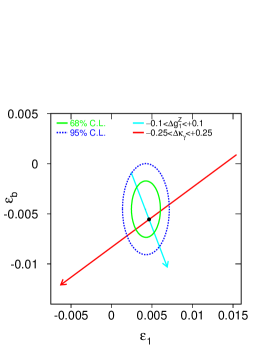
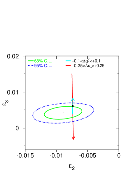
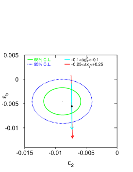
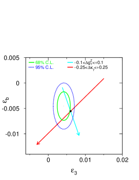
Figure 2: The contours of the $\epsilon$ parameters. The arrows indicate the change of the SM prediction if the coupling parameters $\Delta g^{1}_{Z}$ and $\Delta\kappa_{\gamma}$ are varied according to the direct measurements of LEP 2 and TEVATRON.

are extracted. These parameters are very sensitive to radiative corrections and thus the influence of physics beyond the SM, hence also very sensitive to non-SM TGCs. It is interesting to note that $\epsilon_{2}$ and $\epsilon_{b}$ do not, on the one-loop level, depend on the yet unknown Higgs-mass $m_{H}$. Here $\Delta\rho$ stands for radiative corrections to the $\rho$-parameter [7], $\Delta r_{w}$ describes corrections to the $G_{F}$-$M_{W}$ relation and $\Delta k^{\prime}$ relates $\sin^{2}\theta_{W}^{0}$ to the effective electroweak mixing angle [6]. As the fermion coupling constants depend on the $\epsilon$-parameters one can extract these from the measurements reported in table 1 (except the top-quark mass), which all depend on $g_{V}$, $g_{A}$ or $\sin^{2}\theta_{W}$. A simultaneous fit to all four parameters and in addition to the electromagnetic coupling constant $\alpha_{em}(m_{Z})$, the strong coupling constant $\alpha_{s}(m_{Z})$ and $m_{Z}$ gives the numbers quoted in table 2. The computation of the SM expectations shows that these values are in good agreement with the measured ones, and they are also in good agreement with other recent computations [8, 9]. One finds strong correlations between $\epsilon_{b}$ and $\alpha_{s}$ as well as for $\epsilon_{1}$ and $\epsilon_{3}$. The latter is visible in figure 2, showing the two-dimensional contours of each pair of $\epsilon$-parameters. These contour curves are compared with the evolution of the $\epsilon$-parameters as a function of the TGC coupling constants.

The dependence of the $\epsilon$-parameters on the WWV couplings is shown in the following equations[10, 11, 4] :

$$-\frac{12\pi}{\alpha}\Delta\epsilon_{1} =\left\{\left[\frac{27}{2}-\tan^{2}\theta_{W}\right]\frac{m_{Z}^{2}}{m_{W}^{2}}\ln\frac{\Lambda^{2}}{m_{W}^{2}}+\frac{9}{2}\frac{m_{Z}^{2}m_{H}^{2}}{m_{W}^{4}}\left[\ln\frac{\Lambda^{2}}{m_{H}^{2}}+\frac{1}{2}\right]\right\}\Delta\kappa_{\gamma}$$

$$+\left\{\left[\tan^{2}\theta_{W}-\cot^{2}\theta_{W}\right]-\frac{9}{2}\frac{m_{H}^{2}}{m_{W}^{2}}\left[\ln\frac{\Lambda^{2}}{m_{H}^{2}}+\frac{1}{2}\right]\right\}\Delta g^{1}_{Z}$$ (11)

$$\frac{12\pi}{\alpha}\Delta\epsilon_{2} =\frac{m_{Z}^{2}}{m_{W}^{2}}\ln\frac{\Lambda^{2}}{m_{W}^{2}}\sin^{2}\theta_{W}\Delta\kappa_{\gamma}+\cot^{2}\theta_{W}\ln\frac{\Lambda^{2}}{m_{W}^{2}}\Delta g^{1}_{Z}$$ (12)

$$\frac{12\pi}{\alpha}\Delta\epsilon_{3} =\left\{\left[\cos^{4}\theta_{W}-7\cos^{2}\theta_{W}-\frac{3}{4}\right]\frac{m_{Z}^{2}}{m_{W}^{2}}\ln\frac{\Lambda^{2}}{m_{W}^{2}}-\frac{3}{4}\frac{m_{H}^{2}}{m_{W}^{2}}\left[\ln\frac{\Lambda^{2}}{m_{W}^{2}}+\frac{1}{2}\right]\right\}\Delta\kappa_{\gamma}$$

$$+\left\{10\cos^{2}\theta_{W}+\frac{3}{2}\right\}\ln\frac{\Lambda^{2}}{m_{W}^{2}}\Delta g^{1}_{Z}$$ (13)

$$\Delta\epsilon_{b} =\frac{m_{Z}^{2}m_{t}^{2}}{64\pi^{2}m_{W}^{4}}\ln\frac{\Lambda^{2}}{m_{W}^{2}}\Delta\kappa_{\gamma}$$

$$-\left[\frac{\cot^{2}\theta_{W}}{64\pi^{2}}\frac{m_{Z}^{2}m_{t}^{2}}{m_{H}^{4}}\ln\frac{\Lambda^{2}}{m_{W}^{2}}+\frac{3\cot^{2}\theta_{W}}{32\pi^{2}}\frac{m_{t}^{2}}{m_{W}^{2}}\ln\frac{\Lambda^{2}}{m_{W}^{2}}\right]\Delta g^{1}_{Z}$$ (14)

These expressions are based on the constraints between TGCs quoted earlier. All non-standard contributions are logarithmically divergent. The coupling parameters, that are used here, are defined in dependence on the new physics scale $\Lambda$ and a form factor f coming from the new physics effect, eg.

$$\Delta g^{1}_{Z} =\frac{m_{Z}^{2}}{\Lambda^{2}}f.$$ (15)

Thus the coupling parameters vanish in the limit of a large new physics scale, $\Lambda\rightarrow\infty$. The new physics scale in the following measurement is set to 1 TeV. In addition a Higgs-mass of 300 GeV is assumed.

A fit using equations 11 to 14 and the difference of the measured values of the $\epsilon$-parameters and the ones expected in the SM as shown in table 2 is used to determine the TGC coupling parameters $\Delta g^{1}_{Z}$ and $\Delta\kappa_{\gamma}$. The errors on the SM predictions of the $\epsilon$-parameters are included, neglecting their correlations. The $\chi^{2}$ curves of a fit to each of these coupling constants, setting the other to its SM value of zero, is shown in figure 3. One finds the following results:

$$\Delta g^{1}_{Z} =-0.017\pm 0.018$$ (16)

$$\mathrm{~{}~{}~{}~{}~{}~{}~{}~{}or}$$

$$\Delta\kappa_{\gamma} =0.016\pm 0.019.$$ (17)

If both couplings are allowed to vary in the fit, one finds the contour plot in figure 4. The corresponding numerical values of the TGC-parameters are

$$\Delta g^{1}_{Z} =-0.013\pm 0.027$$

$$\Delta\kappa_{\gamma} =0.005\pm 0.029,$$ (18)

with a correlation of 75.5 percent.

The SM expectation of zero for both parameters agrees well with this measurement. As 1 TeV is the lower limit of the new physics scale and the couplings depend inversely on $\Lambda$, the errors decrease with increasing $\Lambda$. Higher Higgs masses decrease also the errors on the TGC, while a lower Higgs mass increases the error. Assuming a 100 GeV Higgs, the error on $\Delta g^{1}_{Z}$ increases by 1% of the error, while the one-dimensional error on $\Delta\kappa_{\gamma}$ increases to 0.033. The error of 5 GeV on $m_{t}$, as quoted in table 1 has a negligible impact on the result.

The results presented above are more precise than recent direct measurements of the LEP and TEVATRON collaborations [5]: $\Delta g^{1}_{Z}=0.00^{+0.12}_{-0.11}$ and $\Delta\kappa_{\gamma}=0.28^{+0.33}_{-0.27}$. Here the parameters are negatively correlated with -54 percent. The direct measurement is however more suitable for a general test of the TGCs while the indirect measurement tests TGCs only in particular models.

Recent computations [10, 11] parametrise also the dependence of $\epsilon_{b}$ on the coupling constants $\lambda_{\gamma}$ and $g^{5}_{Z}$ giving access to a more general view of the TGC couplings. Computations of the dependence of $\epsilon_{1}$, $\epsilon_{2}$ and $\epsilon_{3}$ on the TGCs $\lambda_{\gamma}$ and $g^{5}_{Z}$ would be most useful to measure also these coupling constants more precisely.

3 Acknowledgements

We are very grateful to S. Riemann for bringing the possibility of the indirect measurement of TGCs to our attention. We thank F.Caravaglios and G.Altarelli for clarifying discussions on the $\epsilon$ parameters and T. Hebbeker, W.Lohmann and T. Riemann for useful comments.

a)           b)

c)           d)

Figure 1: Radiative correction to the decay width of the $\mathrm{Z}^{0}$into fermions, $\mathrm{Z}^{0}$$\rightarrow f\bar{f}$. This process is used to constrain the Higgs-boson and top-quark mass. Graphs a) and b) depend on the WWV coupling constants, while graphs c) and d) depend only on fermion to boson couplings.

parameter	central value	errors
$1/\alpha^{(5)}(m_{Z})$	128.878	0.090
$m_{Z}$	91.1867	0.0021
$\Gamma_{Z}$	2.4939	0.0024
$\sigma_{\mathrm{had}}$	41.491	0.058
$R_{e}$	20.765	0.026
$A_{FB}^{e}$	0.01683	0.00096
${\cal P}_{e}$	0.1479	0.0051
${\cal P}_{\tau}$	0.1431	0.0045
$\sin^{2}\theta_{w}^{\mathrm{eff}}(Q_{\mathrm{fb}})$	0.2321	0.0010
$\sin^{2}\theta_{w}^{\mathrm{eff}}(A_{\mathrm{LR}})$	0.23109	0.00029
$m_{W}$ (LEP2)	80.37	0.09
$m_{W}$ (p$\bar{\mathrm{p}}$)	80.41	0.09
$R_{b}$	0.21656	0.00074
$R_{c}$	0.1735	0.0044
$A_{FB}^{b}$	0.0990	0.0021
$A_{FB}^{c}$	0.0709	0.0044
$A_{b}$	0.867	0.035
$A_{c}$	0.647	0.040
$m_{t}$	173.8	5.0

Table 1: Preliminary electroweak parameters that are used in the fit to the $\epsilon$ parameters. The correlations among the observables in the b and c quark sector as well as the one between $m_{Z}$, $\Gamma_{Z}$, $\sigma_{\mathrm{had}}$, $R_{e}$ and $A^{e}_{FB}$ is taken properly into account. Consult [5] and references therein for details. $m_{t}$ is only used in the Standard Model calculation of the $\epsilon$-parameters.

fit parameter	measured		MSM	correlation matrix
				$\frac{1}{\alpha^{(5)}}$	$\alpha_{s}$	$m_{Z}$	$\epsilon_{1}$	$\epsilon_{2}$	$\epsilon_{3}$	$\epsilon_{b}$
$1/\alpha^{(5)}(m_{Z})$	128.878$\pm$	0.090	-	1.00	0.00	0.00	0.00	-0.07	0.46	0.00
$\alpha_{s}(m_{Z})$	0.1244$\pm$	0.0045	-	0.00	1.00	0.00	-0.45	-0.22	-0.31	-0.62
$m_{Z}$	91.1866$\pm$	0.0021	-	0.00	0.00	1.00	-0.06	-0.01	-0.02	0.00
$\epsilon_{1}\times 10^{3}$	4.2$\pm$	1.2	$4.6\pm 1.1$	0.00	-0.45	-0.06	1.00	0.44	0.80	-0.01
$\epsilon_{2}\times 10^{3}$	$-8.9$$\pm$	2.0	$-7.5\pm 0.3$	-0.07	-0.22	0.00	0.44	1.00	0.26	-0.01
$\epsilon_{3}\times 10^{3}$	4.2$\pm$	1.2	$5.8\pm 0.7$	0.46	-0.31	-0.02	0.80	0.26	1.00	0.00
$\epsilon_{b}\times 10^{3}$	$-4.5$$\pm$	1.9	$-5.8\pm 0.5$	0.00	-0.62	0.00	-0.01	-0.01	0.00	1.00

Table 2: The $\epsilon$ values in the SM and from a fit to the electroweak data summarised in table 1 ($\chi^{2}/Ndf~{}=~{}11.6/11$, probability 39%).

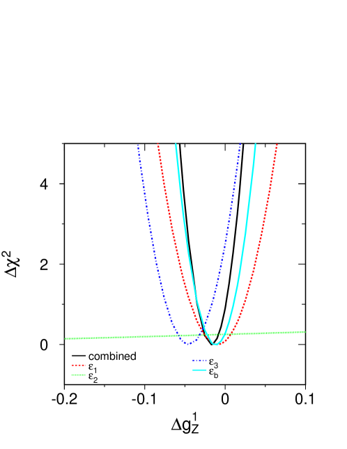
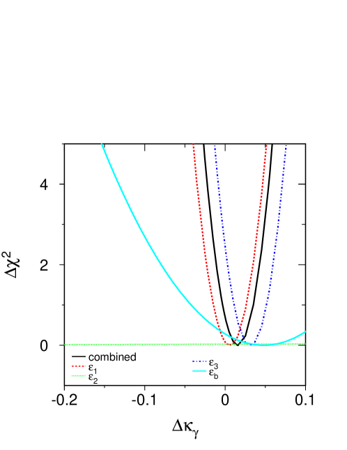
Figure 3: The $\Delta\chi^{2}$ curves for the TGC couplings and the contributions of the different $\epsilon$ parameters. The combined curve is the add up of the single curves taking the correlation coefficients properly into account. The parameter $\epsilon_{2}$ has almost no sensitivity to TGCs.

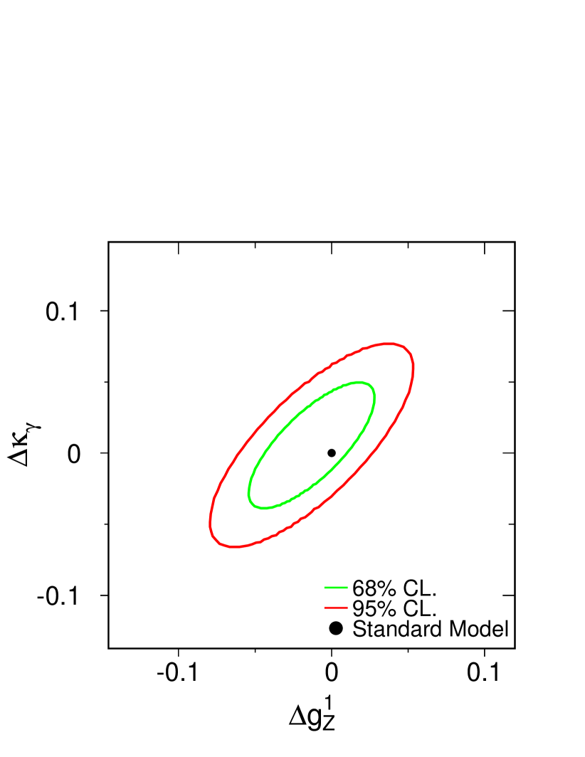
Figure 4: The contour curves for the two dimensional fit, $\Delta g^{1}_{Z}$ versus $\Delta\kappa_{\gamma}$. The dot shows the SM expectation.

References

• [1] G. Gounaris etΒ al., in Physics at LEP 2, Report CERN 96-01 (1996), eds G. Altarelli, T. SjΓΆstrand, F. Zwirner, Vol. 1, p. 525
• [2] S.Β L. Glashow, Nucl. Phys.Β 22 (1961) 579;
S. Weinberg, Phys. Rev. Lett.Β 19 (1967) 1264;
A. Salam, in Elementary Particle Theory, ed. N. Svartholm, Stockholm, Almquist and Wiksell (1968), 367
• [3] A. De Rujula and M. B. Gavela and P. Hernandez and E. Masso, Nucl. Phys. B384 (1992) 3–58
• [4] K. Hagiwara, S. Ishihara, R. Szlapski, and D. Zeppenfeld, Phys. Lett. B 283 (1992) 353, Phys. Rev. D 48 (1993) 2182
• [5] M. W. GrΓΌnewald, Combined Analysis of Precision Electroweak Results, HUB-EP-98/67, invited talk at the ICHEP98 in Vancouver, 1998, to appear in the proceedings
D. Karlen, Experimental status of the Standard Model, invited talk at the ICHEP98 in Vancouver, 1998, to appear in the proceedings
• [6] G. Altarelli and R. Barbieri, Phys. Lett. B253 (1991) 161–167
• [7] M. Veltman, Nucl. Phys. B123 (1977) 89
• [8] G. Altarelli, The Standard electroweak theory and beyond, Preprint hep-ph/9811456, 1998
• [9] M.W. GrΓΌnewald, Experimental tests of the electroweak Standard Model at high energies, Preprint HUB-EP-98/78, 1998
• [10] O. J. P. Eboli and S. M. Lietti and M. C. Gonzalez-Garcia and S. F. Novaes, Phys. Lett. B339 (1994) 119–126
• [11] O. J. P. Eboli and M. C. Gonzalez-Garcia and S. F. Novaes, Indirect constraints on the triple gauge boson couplings from Z $\to$ b anti-b partial width: An Update, Preprint hep-ph/9811388, 1998.
a) Ξ”WW$\mathrm{Z}^{0}$/$\gamma$ $\bar{f}$ $f$Β Β Β Β Β Β Β Β Β  b) ΘWW$\mathrm{Z}^{0}$/$\gamma$ $\bar{f}$ $f$
c) Ξ›W$\mathrm{Z}^{0}$/$\gamma$ $\bar{f}$ $f$Β Β Β Β Β Β Β Β Β  d) Ξ$\mathrm{Z}^{0}$/$\gamma$ $\bar{f}$ $f$