UND-HEP-99-BIG 02

hep-ph/9902315

Heavy Quark Expansion and
Preasymptotic Corrections to Decay Widths
in the ’t Hooft Model

Ikaros Bigi${}^{\>a}$ and Nikolai Uraltsev${}^{\>a,b}$
^aDept. of Physics, Univ. of Notre Dame du Lac, Notre Dame, IN 46556, U.S.A.
^bPetersburg Nuclear Physics Institute, Gatchina, St. Petersburg, 188350, Russia

Abstract

We address nonperturbative power corrections to inclusive decay widths of heavy flavor hadrons in the context of the ’t Hooft model (two-dimensional QCD at $N_{c}\to\infty$), with the emphasis on the ‘spectator-dependent’ effects, i.e. those sensitive to the flavor of the spectator. The summation of exclusive widths is performed analytically using the ’t Hooft equation. We show that the $1/m_{Q}$ expansion of both the Weak Annihilation and Pauli Interference widths coincides with the OPE predictions, to the computed orders. Violation of local duality in the inclusive widths is quantified, and the new example is identified where the OPE prediction and the actual effect are completely saturated by a single final state. The qualitative aspects of quark hadronization emerging from the analysis in the ’t Hooft model are discussed.

Certain aspects of summation of spectator-independent hadronic weak decay widths are given in more detail, which were not spelled out previously. We also give some useful details of the $1/m_{Q}$ expansion in the ’t Hooft model.

PACS numbers: 12.38.Aw, 12.39.Hg, 23.70.+j, 13.35.Dx

1 Introduction

The decays of heavy flavor hadrons $H_{Q}$ are shaped by nonperturbative strong interaction dynamics which, at first sight, completely obscures most of the properties of the underlying weak interactions self-manifest at the quark level. It is suffice to say that the actual hadrons, rather than quarks are observed in the final state. The actual dynamics of confinement in QCD to a large extent remains mysterious. Nevertheless, significant progress has been achieved in describing heavy flavor decays applying the formalism based on Wilson’s operator product expansion (OPE) [2]. In particular, it became possible to quantify the effects of the confining domain on the inclusive decay rates. This theory is in the mature stage now (see Refs. [4, 5] and references therein).

Among the general statements derived for the heavy quark decays, we mention here

$\bullet$ Absence of $\Lambda_{\rm QCD}/m_{Q}$ corrections to all types of fully inclusive decay widths [6, 7].

$\bullet$ The leading nonperturbative corrections arise in order $1/m_{Q}^{2}$ and are given by the expectation values $\mu_{\pi}^{2},\;\mu_{G}^{2}$ of the two heavy quark operators, kinetic and chromomagnetic. While the first effect is universal amounting to the correction $-\mu_{\pi}^{2}/2m_{Q}^{2}$, the Wilson coefficient for the second one depends on the considered process. Both, however, are insensitive to the flavor of the spectator(s) (“flavor-independent” corrections) [6, 7].

$\bullet$ The widths are determined by the short-distance running quark masses $m_{Q}(\mu)$ [9]. These are shielded against uncontrollable corrections from the infrared domain which would otherwise bring in uncertainty $\delta m_{Q}/m_{Q}\sim\Lambda_{\rm QCD}/m_{Q}$.

$\bullet$ The effects sensing the spectator flavor per se, emerge at the level $1/m_{Q}^{3}$ [10, 11, 6]. They are conventionally called Weak Annihilation (WA) in mesons, Weak Scattering (WS) in baryons and Pauli Interference (PI) in both systems. Their magnitudes are given by the expectation values of local four-quark operators.

For practical applications we should keep the following in mind (for a recent dedicated discussion, see Refs. [12, 13, 5]):

– Good control over the perturbative expansion must be established to address power-suppressed effects.

– The consistent Wilsonian OPE requires introducing the separation of “hard” and “soft” scales, with the borderline $\mu$ serving as the normalization point in the effective theory.

– One has to allow, in principle, for short-distance (small-coupling regime) effects that are not directly expandable in the powers of the strong coupling.

– Account must be taken of the fact that the OPE power series are only asymptotic [14], and reconstructing from them the actual Minkowskian observable, generally speaking, potentially leaves out the oscillating (sign-alternating) contributions suppressed, in a certain interval of energies, by only a power of the high momentum scale. This is compounded by the fact that in practice one can typically determine only the first few terms in the power expansion.

The last item in the list is behind the phenomenon of violation of local parton-hadron duality; in many cases it is among the primary factors potentially limiting the accuracy of the theoretical expansion.

In the actual QCD these technical complications are often interrelated. Therefore, it is instructive to investigate the OPE in a simplified setting where these elements can be disentangled. As explained in Ref. [12], this is achieved in QCD formulated in 1+1 dimensions. Additionally, employing the limit $N_{c}\to\infty$ one arrives at the exactly solvable ’t Hooft model where all the features can be traced explicitly. It is important that the ’t Hooft model maintains the crucial feature of QCD – quark confinement – which is often believed to be tightly related to the violation of local duality. Yet in 1+1 dimensions confinement appears already in the perturbative expansion.

The ’t Hooft model has often been used as a theoretical laboratory for exploring various field-theoretic approaches [15]. Most recently the OPE for the inclusive widths and the related sum rules in the heavy flavor transitions [16] were analytically studied in Ref. [12], where a perfect match between the OPE power expansion and the actual asymptotics of the widths was found. The known high-energy asymptotics of the spectrum in the model allowed us to determine the violation of local duality in the inclusive widths at large $m_{Q}$. As expected, it obeyed the general constraints imposed by the OPE. Moreover, at least in the framework of this simplified model, the main features of duality violation could be inferred from the parton-level analysis itself, the working tools of the OPE. The suppression of the duality-violating component in $\Gamma_{H_{Q}}$ was found to be rather strong, with the power of $1/m_{Q}$, however, depending essentially on the particulars of the considered model and the process.

Ref. [12] focussed on flavor-independent effects. To this end it was assumed that the spectator quark $q_{\rm sp}$ has a flavor different from all quarks in the final state, thus ruling out both WA and PI. The OPE analysis of these effects is also straightforward. Nevertheless, they may be of independent interest for several reasons.

First, WA and PI represent power-suppressed and thus purely preasymptotic effect. In such a situation one may expect a later onset of duality and more significant violations of local duality. Since the above effects are numerically enhanced for actual charm and beauty hadrons, studying this question has practical importance.

Figure 1: a) Quark diagram describing the leading quasifree term in the decay width. b) Bare quark diagram for WA.

Another reason to look more closely at the spectator-dependent effects is related to the color-flow considerations usually employed in the context of the large-$N_{c}$ perspective on QCD, and interpreting the OPE predictions in terms of hadronic states. In the case of the quasi-free quark decay width or the WA processes one finds a rather straightforward correspondence between the OPE expressions and the hadronic contributions already in the simplest quark picture where quark allocation over the final state hadrons is unambiguous (such a description is expected to hold at $N_{c}\to\infty$). Let us consider, for example, the free parton decay diagram Fig. 1a. The $\bar{u}d$ pair is in a colorless state and typically has a large momentum $q^{2}\sim m_{b}^{2}$ flowing through it. It is then naturally dual to the contributions from the hadronic resonances in the $V$–$A$ channel (in particular when integrated over $q^{2}$), much in the same way as in ${\rm e}^{+}{\rm e}^{-}$ annihilation or hadronic $\tau$ decays. The $c$ quark together with the spectator antiquark produces another string of hadronic excitation. Furthermore, the interaction between these two hadronic clusters can naturally be small at large $m_{b}$. WA, Fig. 1b, looks even simpler in this respect; we will discuss it in detail later on.

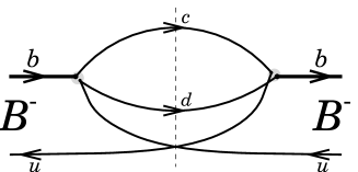
Figure 2: Quark diagram for PI in $B$ meson decays. The weak vertices are broken to show the color flow yielding the leading-$N_{c}$ contribution.

The hadronic picture of the processes underlying PI a priori  is less obvious, Fig. 2. The $\bar{u}$ quark produced in the decay must be slow to interfere with the valence $\bar{u}$. The large momentum here flows through the diquark loop ($cd$) which therefore represents the “hard core” of the process. The practical OPE, effectively, prescribes to replace the propagation of this diquark by a nearly free di-fermion loop, which amounts to evaluating its absorptive part as if the production of the free quarks was considered. Basically, no distinction emerges compared to the color-singlet $\bar{q}q^{\prime}$ pairs in Figs. 1. This may leave one with the feeling of discomfort, for no colored states (in particular, with the diquark content) is present in the physical spectrum. In other words, the diquark configuration per se cannot be dual to the mesonic states at any arbitrary large momentum transfer.

Alternatively, one can combine a “hard” quark from the loop in Fig. 2 with the slow spectator antiquark to have a color-singlet meson-like configuration. However, such a pair naively is not “hard”: at least in the perturbative partonic picture with $p_{\rm sp}\sim m_{\rm sp}\to 0$ its invariant mass vanishes irrespective of $m_{b}$. While such reasoning is clearly of the hand-waving variety, it illustrates nevertheless that interference effects are more subtle.

A more troublesome feature of the interference is also illustrated by the observation made in the early 90s by Shifman [17]. He considered a more general scenario with both charged- and neutral-current type interactions, as described by the effective weak Lagrangian

$${\cal L}=-\frac{G}{\sqrt{2}}\left[a_{1}\,(\bar{c}\gamma_{\mu}(1\!-\!\gamma_{5})b)\,(\bar{d}\gamma^{\mu}(1\!-\!\gamma_{5})u)\,+\,a_{2}\,(\bar{d}\gamma_{\mu}(1\!-\!\gamma_{5})b)\,(\bar{c}\gamma^{\mu}(1\!-\!\gamma_{5})u)\right]\,+\,{\rm H.c.}\;.$$ (1)

The leading (rather than the power-suppressed spectator-dependent) width was addressed. The parton result depends on the color factors $a_{1}$, $a_{2}$ in the following way:

$$\Gamma_{Q}\;\sim\;N_{c}\left(a_{1}^{2}+a_{2}^{2}+\frac{2}{N_{c}}a_{1}a_{2}\right)\;.$$ (2)

On the other hand, the usual counting rules yield the decay amplitudes into the two-meson final states in the form

$${\cal M}\propto\sqrt{N_{c}}\left(a_{1}+\frac{1}{N_{c}}a_{2}\right) D_{s}\pi^{-}$$ for “” states

$${\cal M}\propto\sqrt{N_{c}}\left(a_{2}+\frac{1}{N_{c}}a_{1}\right) \mbox{ ``$DK$'' states},$$ for (3)

where, for illustrative purposes, we call $q_{\rm sp}$ the strange quark to simplify distinguishing between the two different ways to pair the quarks into mesons. (Since we discuss the leading free-parton amplitude, the flavor of the spectator is chosen to be different from all other quarks in the process.) Adopting the rules Eq. (3) one gets

$$\Gamma_{Q}\;\sim\;N_{c}\left(a_{1}^{2}+a_{2}^{2}+\frac{4}{N_{c}}a_{1}a_{2}\right)$$ (4)

more or less independently of the dynamics. While the dependence for the terms $\sim a_{1}^{2}$ and $\sim a_{2}^{2}$ is reproduced, there is a clear mismatch between Eqs. (2) and (4) in the term describing the interference of the two different color amplitudes [17].

There is little doubt that the formal OPE asymptotics must work at arbitrary $N_{c}$. The arguments above might suggest, however, that the onset of duality is delayed for suppressed effects, for example, grow with $N_{c}$.

In reality, we do not think that there is convincing evidence supporting such reservations about applying the OPE to flavor-dependent corrections. To provide an additional justification, we have explicitly analyzed both PI and WA in the ’t Hooft model. We have found complete consistency with the OPE, with the onset of duality largely independent of the details. As a matter of fact, the parton-deduced OPE expression for PI appears to be exact in the chiral limit when all involved quarks (but $Q$) are massless. The resolution of the above paradoxes emerges in a rather straightforward manner as well; we will comment on them in subsequent sections.

We note that we disagree with the claims of the recent paper [18] which found a mismatch between the actual WA width and the OPE-based prediction, relying on numerical computations. We have determined the leading effect analytically and showed it to coincide with the OPE result. We comment on the apparent drawbacks in the analysis of Ref. [18] in Sect. 6.

The paper is organized as follows. After this introduction, in Sect. 2 we sketch the aspects of the ’t Hooft model important for addressing weak decays. In Sect. 3. we analyze the effects of WA at $N_{c}\to\infty$ and analytically compute the large-$m_{Q}$ asymptotics of the corresponding heavy meson weak decay width, with technical details given in Appendix 1. Sect. 4 addresses PI; we analytically compute this width up to terms like $\Gamma_{\!H_{Q}}/m_{Q}^{3}$ and find full agreement with the expressions obtained in the OPE. The effects of local duality violation at large $m_{Q}$ are quantified. The special case – with massless final-state quarks – is identified where duality violation is totally absent from the spectator-dependent part of the width. In Sect. 5 we present a more detailed derivation of the total decay width up to corrections $1/m_{Q}^{3}$ explicitly accounting for nonzero light-quark masses, to demonstrate consistency with the OPE (a detailed description of this analysis had been omitted from Ref. [12]). Sect. 6 comments on the analyses which have claimed observing inapplicability of the OPE predictions based on numerical computations. Sect. 7 comprises conclusions and overlook and outlines our perspective on the problem of OPE and duality violation in the decays of heavy flavor hadrons.

Most technicalities are relegated to Appendices. Appendix 2 collects a number of relations useful in constructing analytic $1/m_{Q}$ expansion in the ’t Hooft model and summing the exclusive widths. In particular, we give simple expressions for the leading terms in the transition amplitudes in Appendix 2.2, perform the differential fixed-$q^{2}$ semileptonic decay width summation up to $1/m_{Q}^{2}$ corrections in Appendix 2.3, prove the OPE prescription for the domain of large $q^{2}$ and demonstrate the proper functional form of the transition amplitudes in Appendix 2.4. The expression for the IW functions in terms of the ’t Hooft eigenfunctions is quoted in Appendix 3. Appendix 4 reports a direct covariant computation of the perturbative radiative corrections performed while working on paper [12]; it shows that the result coincides with what is obtained by summing exclusive decay channels.

2 The ’t Hooft model and heavy quark decays

The ’t Hooft model, the 1+1 QCD with $N_{c}\to\infty$ has been described in many papers [19, 20, 21, 22]. The first dedicated studies of heavy quarks in the ’t Hooft model date back to the early 90s [23, 24]. Recent paper [12] specifically addressed heavy quark decays and the OPE in this model. Here we only recapitulate some basic features.

The Lagrangian has the form

$${\cal L}_{1+1}=-\frac{1}{4g_{s}^{2}}\,G_{\mu\nu}^{a}G_{\mu\nu}^{a}\,+\,\sum\bar{\psi}_{i}(i\not\!\!D-m_{i})\psi_{i}\;,\;\;\;\;iD_{\mu}=i\partial_{\mu}+A_{\mu}^{a}T^{a}\,.$$ (5)

The coupling $g_{s}$ has dimension of mass. With the above normalization of the gauge field, $A_{\mu}$ still has dimension of mass as in $D=4$. The fermion fields $\psi(x)$, however, carry dimension of $m^{1/2}$.

The OPE analysis is carried out universally for arbitrary number of colors, and so far $N_{c}$ is kept finite. Anticipating the large $N_{c}$ limit for the final analysis, we define a parameter $\beta$

$$\beta^{2}\;=\;\frac{g_{s}^{2}}{2\pi}\,\left(N_{c}-\frac{1}{N_{c}}\right)\;,$$ (6)

that remains finite at $N_{c}\to\infty$. It plays the role of the nonperturbative scale $\Lambda_{\rm QCD}$.

Following the actual Standard Model, we choose the weak decay interaction of the current-current form. Since in $D=2$ the axial current is related to the vector one, $J_{\mu}^{A}=\epsilon_{\mu\nu}J_{\nu}^{V}$, we simply consider the $V$$\times$$V$ interaction:

$${\cal L}_{\rm weak}\;=\;-\frac{G}{\sqrt{2}}\,(\bar{q}\gamma_{\mu}Q)\,(\bar{\psi}_{a}\gamma^{\mu}\psi_{b})\;+\;{\rm H.c.}\;,$$ (7)

where the dimensionless $G$ is an analogue of the Fermi constant. For semileptonic decays $\psi_{a,b}$ are colorless (leptonic) fields. In what follows our main interest lies in nonleptonic decays with $\psi_{a,b}$ being the quark fields. To make the notations more transparent, we adhere to the cases of interest in actual QCD and denote the $\psi$ fields as $u$ and $d$ quarks, while $Q$ will be a synonym of the $b$ quark, and $q$ called $c$ quark (whether we chose $m_{q}\gg\Lambda_{\rm QCD}$ or consider $m_{q}\mathrel{\hbox to0.0pt{\lower 3.0pt\hbox{\hskip 0.0pt$\sim$}\hss}\raise 1.0pt\hbox{$<$}}\Lambda_{\rm QCD}$). The spectator quark $q_{\rm sp}$ can be either $u$ or $d$ (for studying WA or PI), or different in flavor from both.

To address inclusive widths of a heavy flavor hadron $H_{Q}$ one considers the forward transition amplitude appearing in the second order in the decay interaction [10]:

$$\Gamma_{H_{Q}}\;=\;2\,{\rm Im}\,\int{\rm d}^{D}x\,\frac{1}{2M_{H_{Q}}}\langle H_{Q}|\,i\,T\left\{{\cal L}_{\rm weak}(x){\cal L}_{\rm weak}^{\dagger}(0)\right\}|H_{Q}\rangle\;.$$ (8)

In the limit $N_{c}\to\infty$, with $H_{Q}$ being the mesonic $(Q\bar{q}_{\rm sp})$ states, factorization of the amplitudes holds, which takes the following form for the transition operator:

$$\int{\rm d}^{D}x\,\langle H_{Q}|\,i\,T\left\{{\cal L}_{\rm weak}(x){\cal L}_{\rm weak}^{\dagger}(0)\right\}|H_{Q}\rangle\;=\;\frac{G^{2}}{2}\,\int{\rm d}^{D}x\,T^{\mu\nu}(x)\,\Pi_{\mu\nu}(x)\;,$$ (9)

where we have introduced the “semileptonic” $T_{\mu\nu}$ and “hadronic” $\Pi_{\mu\nu}$ tensors:

$$\Pi_{\mu\nu}(x)\; = \;\langle 0|i\,T\left\{\bar{d}(x)\gamma_{\mu}u(x)\,\bar{u}(0)\gamma_{\nu}d(0)\right\}|0\rangle\;,$$ (10)

$$T^{\mu\nu}(x)\; = \;\langle H_{Q}|i\,T\left\{\bar{q}(x)\gamma^{\mu}Q(x)\,\bar{Q}(0)\gamma^{\nu}q(0)\right\}|H_{Q}\rangle\;.$$ (11)

The Cutkosky rules then yield

$$\Gamma_{H_{Q}}\;=\;G^{2}\,\frac{1}{M_{H_{Q}}}\,\int{\rm d}^{D}x\,{\rm Im}\,T^{\mu\nu}(x)\,{\rm Im}\,\Pi_{\mu\nu}(x)\;.$$ (12)

The factorized representation of the decay width holds only at $N_{c}\to\infty$ where the momenta of the $\psi_{a}\bar{\psi}_{b}$-pair and $(q\bar{q}_{\rm sp})$ become observables separately. In other words, in this limit there is a rigid quark allocation over the particular hadronic final state and factorization of the corresponding amplitudes, and there is no “cross-talk” between them. Yet, Eq. (12) represents a certain observable at arbitrary $N_{c}$ and, as such, enjoys the full rights of being studied regardless of the details of the model. In particular, at large energy release it is a short-distance observable and can be subjected to an OPE anatomy. In what follows we will discuss this quantity and refer to it as the inclusive decay width as motivated by the large-$N_{c}$ limit.

It is worth noting at this point that the qualitative difference between nonleptonic and semileptonic inclusive widths disappears for $N_{c}\to\infty$. The nonleptonic width is given directly in terms of the differential semileptonic distributions $\frac{{\rm d}\Gamma^{\rm sl}}{{\rm d}q^{2}}$ (though, in $D=2$ one may have to consider the decays with massive leptons as well). Indeed, with $m_{u}=m_{d}$ as an example, one has (in the momentum representation)

$$\Pi_{\mu\nu}(q^{2})\;=\;\frac{1}{\pi}\>\Pi(q^{2})\,\left(q^{2}\delta_{\mu\nu}-q_{\mu}q_{\nu}\right)\;,\qquad\rho(q^{2})\;\equiv\;-\frac{1}{\pi}\>\mbox{Im}\>\Pi(q^{2})\;,$$ (13)

and

$$\Gamma_{H_{Q}}^{\rm nl}\;=\;\int\,{\rm d}q^{2}\>\rho(q^{2})\,\Gamma_{\rm sl}(q^{2})\qquad\mbox{with }\;\,\Gamma_{\rm sl}(q^{2})\;=\;\frac{1}{\rho_{\rm lept}(q^{2})}\,\frac{{\rm d}\Gamma_{H_{Q}}^{\rm sl}}{{\rm d}q^{2}}\;.$$ (14)

In $D=2$ the correlator of vector currents for massless quarks is known exactly and is very simple:

$$\Pi(q^{2})\;=\;\frac{N_{c}}{q^{2}}\;,\qquad\rho(q^{2})\;=\;N_{c}\,\delta(q^{2})\;.$$ (15)

With nonzero quark masses the spectral density shifts upward, to the mass scale $\sim\beta m$ or $m^{2}$. A high-energy tail in $\rho$ also appears $\sim N_{c}(m_{u}^{2}+m_{d}^{2})/q^{4}$. This will be quantified in Sect. 3.

More specific for heavy quark decays is the “semileptonic” part $T_{\mu\nu}(x)$, Eq. (11). The general color counting rules determine its $N_{c}$ behavior:

$$T_{\mu\nu}(x)\;\sim\;N_{c}^{1}\;.$$ (16)

Such a leading contribution, however, can arise only with the vacuum as intermediate state; all other contributions scale as $N_{c}^{0}$, or even are further suppressed. The vacuum intermediate state is possible only when the decay quark $q$ has the same flavor as $q_{\rm sp}$. This is the effect belonging to WA. Therefore, one has

$$\Gamma_{\rm nl}^{\rm WA}\; \sim\;N_{c}^{2}\;,\qquad\;\Gamma_{\rm sl}^{\rm WA}\; \sim\;N_{c}^{1}$$ (17)

$$\Gamma_{\rm nl}\; \sim\;N_{c}^{1}\;,\qquad\;\Gamma_{\rm sl}\; \sim\;N_{c}^{0}\qquad\mbox{ at }q\neq q_{\rm sp}\;.$$ (18)

Since WA is a leading-$N_{c}$ effect, vacuum factorization saturates $T_{\mu\nu}^{\rm WA}$ at $N_{c}\to\infty$, and the effect takes the simplest form. This is the subject of the next section.

On the other hand, the “usual” non-spectator widths are formally subleading in $N_{c}$ (even though they may yield the dominant contribution to the decay width for a particular type of the heavy meson). For such amplitudes the naive factorization does not hold, and the explicit expressions take a far less trivial form. In the context of the OPE, this emerges as “color-disfavored” structure of the resulting local operators, so that a priori the factorization cannot be applied to evaluate their expectation values [12].

In the limit $N_{c}\to\infty$ the spectrum of $1$+$1$ QCD consists of mesonic quark-antiquark bound states which are stable under strong interactions. The meson masses are given by eigenvalues of the ’t Hooft equation

$$M^{2}_{n}\varphi_{n}(x)=\left[\frac{m_{1}^{2}-\beta^{2}}{x}+\frac{m_{2}^{2}-\beta^{2}}{1-x}\right]\varphi_{n}(x)-\beta^{2}\int_{0}^{1}{\rm d}y\,\frac{\varphi_{n}(y)}{(y-x)^{2}}\;,$$ (19)

where $m_{1,2}$ are the bare quark masses of the constituents, and the integral is understood in the principal value prescription. The solutions to the equation are the light-cone wave functions $\varphi(x)$, with $x\,\in\,[0,1]$ having the meaning of the portion of momentum carried by the (first) quark. They are singular at $x=0$ and $x=1$ where their behavior is given by $x^{\gamma_{0}}$ and $(1-x)^{\gamma_{1}}$, respectively, with $\gamma_{0,1}$ defined by the following conditions:

$$\frac{\pi\gamma_{0}}{{\rm tan}\pi\gamma_{0}}=-\frac{m_{1}^{2}-\beta^{2}}{\beta^{2}}\,\,,\;\;\;\;\frac{\pi\gamma_{1}}{{\rm tan}\pi\gamma_{1}}=-\frac{m_{2}^{2}-\beta^{2}}{\beta^{2}}\,.$$ (20)

In full analogy with nonrelativistic quantum mechanics, the eigenfunctions $\varphi_{n}$ form a basis (complete in the physical space):

$$\int_{0}^{1}{\rm d}x\>\varphi_{n}(x)\varphi_{k}(x)\;=\;\delta_{nk}\;,\qquad\;\sum_{n}\,\varphi_{n}(x)\varphi_{n}(y)\;=\;\delta(x-y)\;.$$ (21)

The weak decay constant of a particular meson is given by

$$f_{n}\;=\;\sqrt{\frac{N_{c}}{\pi}}\,\int_{0}^{1}{\rm d}x\>\varphi_{n}(x)\;,$$ (22)

and the polarization tensor of vector currents (at $m_{u}=m_{d}$) takes the form

$$\Pi(q^{2})\;=\;\pi\sum_{n}\,\frac{f_{n}^{2}}{q^{2}-M_{n}^{2}}\;,\qquad\rho(q^{2})\;=\;\pi\sum_{n}\,f_{n}^{2}\,\delta\left(q^{2}-M_{n}^{2}\right)\;.$$ (23)

As mentioned above, at $m_{u}=m_{d}=0$ one has $M_{0}=0$ and $f_{0}=\sqrt{N_{c}/\pi}$, but for all excitations $f_{n}=0$.

The transition formfactors between two mesonic states that define the non-annihilation widths for large $N_{c}$, are of order $N_{c}^{0}$. Since the weak quark currents $\bar{Q}q$ are formally of order $N_{c}^{1}$, these formfactors are “subleading” in the same sense as was discussed previously and, in general have a more complicated form corresponding to the first order correction in the $1/N_{c}$ expansion [21, 22].

3 Weak Annihilation at $N_{c}\to\infty$

WA in the decays of heavy mesons becomes possible when one of the quarks produced in the weak vertex has the same flavor as the spectator antiquark. We assume $q=q_{\rm sp}$, in our notations. As detailed in the preceding section, in this case there is a single contribution to the transition tensor $T_{\mu\nu}$ proportional to $N_{c}$ and leading to $\Gamma_{H_{Q}}\sim N_{c}^{2}$. This is associated with the vacuum intermediate state, and is given by

$$T_{\mu\nu}(x)\;=\;i\,{\rm e\,}^{-iPx}\vartheta(x_{0})\>\langle H_{Q}|\,\bar{Q}\gamma_{\nu}q\,|0\rangle\langle 0|\,\bar{q}\gamma_{\mu}Q\,|H_{Q}\rangle\;,$$ (24)

(with $P_{\alpha}$ denoting the momentum of the decaying heavy flavor hadron $H_{Q}$), so that, in the momentum representation,

$${\rm Im}\,T_{\mu\nu}(q)\;=\;\frac{1}{2}(2\pi)^{D}\,\delta^{D}(P-q)\>\langle H_{Q}|\,\bar{Q}\gamma_{\nu}q\,|0\rangle\langle 0|\,\bar{q}\gamma_{\mu}Q\,|H_{Q}\rangle\;.$$ (25)

This expression is valid in arbitrary dimension for any choice of the weak current – in general, one only must replace $\bar{Q}\gamma_{\mu}q$ by the appropriate quark bilinear. Therefore, at $N_{c}\to\infty$ one has

$$\Gamma^{\rm WA}_{H_{Q}}\;=\;G^{2}\>\frac{1}{2M_{H_{Q}}}\,\langle H_{Q}|\,\bar{Q}\gamma_{\mu}q\,|0\rangle\langle 0|\,\bar{q}\gamma_{\nu}Q\,|H_{Q}\rangle\>{\rm Im}\,\Pi_{\mu\nu}\!\left(M_{H_{Q}}^{2}\right)\;,$$ (26)

which is illustrated in Fig. 3. It can be traced that the OPE corresponds to the same expression if the expectation values of all the higher-dimension four-quark operators reduce to their vacuum factorized values (for earlier discussion of WA in a similar context, see, Ref. [25]). The latter formally holds, in turn, at $N_{c}\to\infty$.

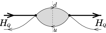
Figure 3: WA correction to the inclusive decay width in the large-$N_{c}$ limit. Shaded loop depicts the exact polarization operator.

In $D=2$ for pseudoscalar $H_{Q}$ one has $\langle 0|\,\bar{q}\gamma_{\mu}Q\,|H_{Q}\rangle=if_{H_{Q}}\epsilon_{\mu\nu}P_{\nu}$. For simplicity, we will further limit ourselves by the case $m_{u}=m_{d}$. Then

$$\Gamma^{\rm WA}_{H_{Q}}\;=\;\frac{G^{2}}{2}\>f_{H_{Q}}^{2}M_{H_{Q}}^{3}\,\rho(M_{H_{Q}}^{2})\;.$$ (27)

Strictly speaking, in practical applications of the OPE, $\Pi_{\mu\nu}$ itself is usually likewise expanded in $1/m_{Q}^{2}$. Also, the deviation of $M_{H_{Q}}^{2}$ from $m_{Q}^{2}$ and/or the values of $f_{H_{Q}}$ are expanded around their asymptotic values at $m_{Q}\to\infty$. Therefore, the sensible check of duality for practical OPE in WA in the framework of the large-$N_{c}$ approximation is only comparison of the actual behavior of ${\rm Im}\,\Pi(q^{2})$ at large $q^{2}$ with its OPE expansion obtained from the deep Euclidean domain.

For massless $u$ and $d$ quarks, the exact polarization operator of the vector currents is given by Eq. (15); the WA width, therefore, vanishes. A non-zero result is obtained if one considers a scalar (pseudoscalar) polarization operator, or if $m_{u}$ or $m_{d}$ do not vanish. The absorptive part $\rho(q^{2})$ is saturated by the comb of narrow resonances with heights $\sim N_{c}$ and widths $\sim 1/N_{c}$. Therefore, the formal limit $N_{c}\to\infty$ requires an alternative to point-to-point comparison of the actual hadronic probabilities with the parton-calculated, or OPE-improved short-distance expansion, even at arbitrary large energies. This implies a certain smearing procedure for the actual hadronic probabilities.

Note that, according to Eq. (26) the width – however singular it is – always remains integrable around the resonances (see also the discussion below, Eqs. (28), (29-33)). By virtue of the dispersion relations the integral of the decay width is expressed via the transition amplitude in the complex plane. This amplitude is regular even in the formal limit $N_{c}\to\infty$ when the resonances become infinitely narrow.

Smearing enters naturally when one considers the ‘imaginary’ part $\frac{1}{2i}\!\left[\Pi(s)\!-\!\Pi(s^{*})\right]$ at complex $s$, somewhat away from the physical cut at $s>0$. According to a dispersion relation it amounts to averaging the physical cross section $R(s)$ with a specific weight,

$$\frac{1}{2i}\left[\Pi(s)-\Pi(s^{*})\right]\;=\;\frac{1}{\pi}\,\int\,{\rm d}\tilde{s}\>\frac{\Delta}{(\tilde{s}-s_{0})^{2}+\Delta^{2}}\>R(\tilde{s})\;,\qquad\;s=s_{0}+i\Delta\,.$$ (28)

One can also use different choices of the smearing function having singularities away from the physical cut.

A similar procedure, in principle, is required for the inclusive decays of heavy flavors. Strictly speaking, one must introduce the complex variable $\omega$ to study the analytic properties of the transition amplitude in question [25, 13, 12]:

$${\cal A}(\omega)\;=\;\int\,d^{D}x\;{\rm e}\,^{-i\omega(vx)}\>\langle H_{Q}|\,i\,T\left\{{\cal L}_{\rm weak}(x){\cal L}_{\rm weak}^{\dagger}(0)\right\}|H_{Q}\rangle\;.$$ (29)

It can be visualized as the transition amplitude governing the total (weak) cross section of the scattering of a fictitious spurion particle $S$ on the heavy quark,

$$S(q)+H_{Q}(p)\;\to\mbox{ light hadrons }\;,$$ (30)

or the weak decay width in the process

$$Q\;\to\mbox{ quarks (leptons) }+\>S\;.$$ (31)

Such processes would appear if the weak decay Lagrangian is modified from, say the conventional four-fermion form to the “four-fermion + spurion” interaction,

$${\cal L}_{\rm weak}(x)\;\to\;S(x)\,{\cal L}_{\rm weak}(x)\;.$$ (32)

For simplicity, it is convenient to assume, as in Eq. (29) that the spurion field does not carry spacelike momentum.

The amplitude ${\cal A}(\omega)$ has the usual analytic properties, and the discontinuity across the physical cut at which the point $\omega=0$ is located, describes the total decay width we are interested in. The OPE for the inclusive widths relies on the fact that the short-distance expansion of ${\cal A}(\omega)$ runs in $1/(\omega-E_{r})$ and can be applied near the physical point $\omega=0$ exactly as in $\rm e^{+}e^{-}$ annihilation near a positive value of $s\gg\Lambda_{\rm QCD}^{2}$. ($E_{r}$ denotes energy release.) To the same extent, in principle, a certain smearing can be required if the hadronic probabilities still exhibit the resonance structure.

Thus, there is no theoretical peculiarity in the asymptotic applications of the OPE for nonleptonic widths. It does not create a conceptual difference to perform a short-distance expansion of a single quark Green function (semileptonic widths or deep inelastic scattering), the product of two Green functions ($\rm e^{+}e^{-}$ annihilation) or the product of three quark Green functions (the nonleptonic widths).

Alternatively, smearing in $\omega$ can be phrased as smearing over the interval of $m_{Q}$. Indeed, in the heavy quark limit the amplitudes depend on just the combination $m_{b}-\omega$,

$${\cal A}(\omega,m_{Q})\;\simeq{\cal A}(0,m_{Q}-\omega)$$ (33)

(there are power corrections to this relation associated with explicit mass effects in the initial state). Therefore, in practical terms one can phrase the smearing as an averaging over the interval of the heavy quark mass, which may look more transparent.

After this general digression, we now return to specifically WA in two-dimensional QCD. It is commonly accepted that, for the two-point current correlators, both at $N_{c}\to\infty$ or finite $N_{c}$, the properly averaged absorptive hadronic parts asymptotically coincide with the leading OPE expression given by the free quark diagram. As was mentioned above, for massless quarks this property holds identically for vector and axial currents. For the scalar current the asymptotic correspondence in the ’t Hooft model has been illustrated already in Ref. [20] (for a recent discussion and earlier references, see Ref. [26]). For the WA width, however, we need the $m_{u,d}$-suppressed effects. The OPE in $D=2$ yields at $m_{u}\!=\!m_{d}\!=\!m$ (for arbitrary $N_{c}$)

$$\Pi(q^{2})=N_{c}\!\left[\frac{1}{q^{2}}\!+\!\frac{2m^{2}}{q^{4}\sqrt{1\!-\!\frac{4m^{2}}{q^{2}}}}\ln{\frac{\sqrt{1\!-\!\frac{4m^{2}}{q^{2}}}\!+\!1}{\sqrt{1\!-\!\frac{4m^{2}}{q^{2}}}\!-\!1}}\right]-\frac{2\pi\langle 0|{m_{u}\bar{u}u\!+\!m_{d}\bar{d}d}|0\rangle}{q^{4}}+{\cal O}\!\left(\frac{m^{2}\ln{q^{2}}}{q^{6}}\right)\!,$$

$$\rho(q^{2})\;=\;N_{c}\,\frac{2m^{2}}{q^{4}}\frac{1}{\sqrt{1-\frac{4m^{2}}{q^{2}}}}\,+\,2\pi\langle 0|m_{u}\bar{u}u+m_{d}\bar{d}d|0\rangle\,\delta^{\prime}(q^{2})\;+\;{\cal O}\left(\frac{m^{2}}{q^{6}}\right)\;,$$ (34)

where the first term in both equations is just the free quark loop. There is little reason to doubt the OPE for the subleading terms either. Nevertheless, it is instructive to give here the direct derivation of the next-to-leading term $\sim(m_{u}^{2}+m_{d}^{2})/q^{4}$ in $\rho(q^{2})$ directly from the ’t Hooft equation.

We follow here the approach of Ref. [12] based on sum rules. In the context of the Euclidean polarization operator similar considerations ascend to the earliest papers on the model, Refs. [20, 21]. To simplify the expressions, we will suppress the explicit powers of $N_{c}$ which enter in a trivial way, and usually will also omit the mass scale factor $\beta$, assuming that all energies are measured in units of $\beta$. Then Eqs. (22), (23) take the form

$$\Pi(q^{2})\;=\;\sum_{n}\,\frac{c_{n}^{2}}{q^{2}-M_{n}^{2}}\;,\qquad\rho(q^{2})\;=\;\sum_{n}\,c_{n}^{2}\,\delta\left(q^{2}-M_{n}^{2}\right)$$ (35)

with

$$c_{n}\;=\;\int_{0}^{1}\,{\rm d}x\>\varphi_{n}(x)\;.$$ (36)

The completeness of eigenstates yields

$$\sum_{n}\,c_{n}^{2}\;=\;\sum_{n}\,\int_{0}^{1}\,{\rm d}x\,{\rm d}y\>\varphi_{n}(x)\varphi_{n}(y)\;=\;1\;.$$ (37)

On the other hand, integrating the ’t Hooft equation from $0$ to $1$ we get

$$c_{n}\;=\;\int_{0}^{1}\,{\rm d}x\;\varphi_{n}(x)\;=\;\frac{1}{M_{n}^{2}}\,\int_{0}^{1}\,{\rm d}x\;\left(\frac{m_{d}^{2}}{x}+\frac{m_{u}^{2}}{1-x}\right)\,\varphi_{n}(x)\;.$$ (38)

Therefore, we get the second sum rule

$$\sum_{n}\,M_{n}^{2}c_{n}^{2}\;=\;\sum_{n}\,\int_{0}^{1}{\rm d}x\;\varphi_{n}(x)\int_{0}^{1}{\rm d}y\left(\frac{m_{d}^{2}}{y}+\frac{m_{u}^{2}}{1\!-\!y}\right)\,\varphi_{n}(y)\,=\,\int_{0}^{1}{\rm d}x\left(\frac{m_{d}^{2}}{x}+\frac{m_{u}^{2}}{1\!-\!x}\right)\,.$$ (39)

The integral logarithmically diverges at $x\to 0$ and $x\to 1$, which corresponds to the behavior

$$\Pi(q^{2})\;\stackrel{{\scriptstyle q^{2}\to\infty}}{{\simeq}}\;\frac{1}{q^{2}}-\frac{m_{u}^{2}+m_{d}^{2}}{q^{4}}\ln{\frac{q^{2}}{m^{2}}}+{\cal O}\left(\frac{1}{q^{4}}\right)$$ (40)

given by the free quark diagram, Eq. (34). The divergence of the sum in Eq. (39) is associated with the high excitations $n$. Therefore, quantifying the divergence allows one to determine the asymptotic behavior of $c_{n}^{2}$.

To render the sum in Eq. (39) finite we must introduce an ultraviolet regularization. For the logarithmic divergence the exact way is not essential – one is to add a hard cutoff factor $\vartheta(\Lambda^{2}\!-\!M_{n}^{2})$. For analytic computations the Borel-type regularization by the factor ${\rm e}^{-M_{n}^{2}/\Lambda^{2}}$ is usually convenient.

For the regularized sums (we mark them with the superscript $\Lambda$) the completeness condition is modified,

$${\sum_{n}}^{\Lambda}\,\varphi_{n}(x)\varphi_{n}(y)\;=\;G(x,y;\Lambda)\;,$$ (41)

and the Green function $G$ becomes a “finite-width” $\delta$-like distribution with the width

$$\Delta\;\sim\;\frac{1}{\Lambda^{2}}\;.$$ (42)

This regularizes the sum in Eq. (39):

$$\sum_{M_{n}^{2}<\Lambda^{2}}\,M_{n}^{2}c_{n}^{2}\;=\;\int_{0}^{\Lambda^{2}}\,q^{2}{\rm d}q^{2}\>\rho(q^{2})\;=\;\int_{0}^{1}\,{\rm d}x\,{\rm d}y\;\left(\frac{m_{d}^{2}}{x}+\frac{m_{u}^{2}}{1-x}\right)\,G(x,y;\Lambda)\;=$$

$$=\;\left(m_{u}^{2}+m_{d}^{2}\right)\left(\ln{\Lambda^{2}}\>+\>\mbox{const}\right)\;.$$ (43)

One has, for instance, for the sum over an interval of highly excited states

$$\int_{\Lambda_{1}^{2}}^{\Lambda_{2}^{2}}\,q^{2}{\rm d}q^{2}\>\rho(q^{2})\;=\;\sum_{\Lambda_{1}^{2}<M_{n}^{2}<\Lambda_{2}^{2}}\,M_{n}^{2}c_{n}^{2}\;=\;\left(m_{u}^{2}+m_{d}^{2}\right)\ln{\frac{\Lambda_{2}^{2}}{\Lambda_{1}^{2}}}\>+\>{\cal O}\left(\frac{1}{\Lambda^{2}}\right)\;.$$ (44)

The sum rule (43) proves that the asymptotics of the smeared ${\rm Im}\,\Pi(q^{2})$ coincides with the free quark loop result through terms $m^{2}/q^{4}$. It is easy to see that the nontrivial corrections in the OPE also emerge only with higher-order terms in $1/q^{2}$. Note that Eqs. (43-44) hold both for light ($m\ll\beta$) and heavy ($m\gg\beta$) quarks. However, for the asymptotics to start, the condition $\Lambda\gg m_{u,d}$ must be observed.

Since $J_{\mu}^{5}=\epsilon_{\mu\nu}J_{\nu}$ and using equation of motion $\partial_{\mu}J_{\mu}^{5}=(m_{u}\!+\!m_{d})\bar{u}i\gamma_{5}d$, by the same token we showed the leading-order duality between the hadronic saturation and the partonic expression for the absorptive part of the pseudoscalar current. A direct derivation in the same approach is described in Appendix 1.

As expected, for large $M_{n}$ one finds the residues $c_{n}\sim m_{u,d}$. Let us note that for light quarks $c_{n}$ are only linear in $m_{q}$: since for light quarks $\varphi_{n}(x)\sim x^{m_{u}}$ at $x\to 0$ (and likewise at $x\to 1$), the end points of integration in Eq. (38) bring in the $1/m_{q}$ enhancement.

Combining the sum rule Eq. (43) with the asymptotics of the ’t Hooft eigenvalues

$$M_{n}^{2}\;\simeq\;\beta^{2}\pi^{2}\,n\;,$$

we obtain

$$c_{n}^{2}\;\simeq\;\pi^{2}\,\beta^{2}\frac{m_{u}^{2}+m_{d}^{2}}{M_{n}^{4}}\;\simeq\;\frac{m_{u}^{2}+m_{d}^{2}}{\pi^{2}\,\beta^{2}\,n^{2}}\;.$$ (45)

Again, these asymptotics are valid if “averaged” over an interval of $n$.

It must be noted that the explicit constant in Eq. (42) is not important. A more detailed derivation of the large-$\Lambda$ asymptotics uses the semiclassical expansion of the ’t Hooft wavefunctions. We show in Appendix 1 that the domain of integration where $x<\frac{1}{\Lambda^{2}}$ or $y<\frac{1}{\Lambda^{2}}$ yields only a finite contribution to the integral in Eq. (43) (and likewise in the vicinity of $x=1$ or $y=1$). At the same time, in the domain $x,y\,\gg\,\frac{1}{\Lambda^{2}}$ the approximation $G(x,y;\Lambda)=\delta(x-y)$ is applicable.

With the relation for the WA width Eq. (26), the comparison of Eq. (44) and the OPE asymptotics Eq. (34) demonstrates that the smeared width in the ’t Hooft model coincides with the OPE width at least through terms $m_{u,d}^{2}/m_{Q}^{2}$.

4 Pauli Interference

In this section we address the effect of interference in the weak decay width of the heavy mesons. As explained in the Introduction, it has an independent interest. Similar to the partonic free-quark decay width, PI is a ‘subleading’ $1/N_{c}$ effect, with $\Gamma^{\rm PI}\sim N_{c}$ rather than $N_{c}^{2}$. Therefore, the expressions for the amplitudes are not as trivial as for WA. Nevertheless, it is not difficult to demonstrate that, again, the quark-based OPE predictions coincide with the actual hadronic widths.

To incorporate PI we must have the flavor of the antiquark produced in the decay of virtual $W$ coinciding with the flavor of the spectator; we shall call it $u$. Moreover, the weak decay Lagrangian must contain two different color structures to have PI at the same order in $N_{c}$ as the free partonic width. So, we adopt, for simplicity,

$${\cal L}_{\rm weak}\;=\;-\frac{G}{\sqrt{2}}\,\left(\,a_{1}(\bar{c}\gamma_{\mu}b)\,(\bar{d}\gamma^{\mu}u)\;+\;a_{2}(\bar{d}\gamma_{\mu}b)\,(\bar{c}\gamma^{\mu}u)\,\right)\;+\;{\rm H.c.}\;,$$ (46)

where, again for notational transparency, we identified $Q$ with $b$ and called $q$ by $c$.

In this case the decay width has three terms,

$$\Gamma_{H_{Q}}\;=\;\frac{G^{2}}{2}N_{c}\,\left(\,a_{1}^{2}\Gamma_{1}+a_{2}^{2}\Gamma_{2}+2a_{1}a_{2}\Gamma_{12}\right)\;,$$ (47)

where $\Gamma_{1}$ and $\Gamma_{2}$ are ${\cal O}(N_{c}^{0})$. Clearly, $\Gamma_{1}(m_{b},m_{c},m_{u},m_{d})=\Gamma_{2}(m_{b},m_{d},m_{u},m_{c})$ holds.

The asymptotics of the non-interference width $\Gamma_{1}$ ($\Gamma_{2}$) for the ’t Hooft model was calculated in Ref. [12] and shown to be given by the OPE one. Now we address the analogous question for $\Gamma_{12}$.

The leading (in $m_{Q}$) contribution to the decay width described by the free parton diagram in Fig. 1a suggests that $\Gamma_{12}\sim 1/N_{c}$. For example, for usual $V$–$A$ interaction in $D=4$ one would have

$$\Gamma_{12}^{\rm parton}\;=\;\frac{1}{N_{c}}\,\Gamma_{1}^{\rm parton}\;=\;\frac{1}{N_{c}}\,\Gamma_{2}^{\rm parton}$$ (48)

(the explicit factor depends on the Lorentz structure of ${\cal L}_{\rm weak}$). Such $N_{c}$-subleading effects are rather complicated. This suppression, however, is not always present [27]. As discussed earlier, invoking the spectator quark through the spectator-dependent effects like WA or PI can bring in an $N_{c}$-enhancement by effectively eliminating the generic $1/N_{c}$ suppression of the free quark width. As a result, at the price of a power suppression in $m_{Q}$ one can have the $N_{c}$-unsuppressed manifestation of the interference of the two color amplitudes in ${\cal L}_{\rm weak}$,

$$\Gamma_{12}^{\rm(PI)}\;\sim\;{\cal O}\left(N_{c}^{0}\right)\;.$$ (49)

Thus, on the one hand, studying PI allows one to address the interference of the color amplitudes in a straightforward way relying on the $1/N_{c}$ expansion. On the other hand, considering the term $\sim a_{1}a_{2}$ in the decay width in the limit $N_{c}\to\infty$ automatically singles out the power-suppressed effect of PI. This goes in contrast with the usual situation where isolating PI formally requires subtracting the decay width of the similar heavy flavor hadron with the spectator(s) having the same mass but with the flavor which is sterile in weak interactions.

The simple quark diagram describing PI is shown in Fig. 2. To leading order it generates the operator

$$\hat{\Gamma}^{\rm PI}\;=\;-2a_{1}a_{2}\frac{G^{2}}{2K}\left\{\left(1-\frac{m_{c}^{2}+m_{d}^{2}}{m_{Q}^{2}}\right)(\bar{b}\gamma_{\mu}\gamma_{5}u)\,(\bar{u}\gamma_{\mu}\gamma_{5}b)\;-\right.$$

$$\left.-\;\frac{2m_{c}m_{d}}{m_{Q}^{2}}\,\left[(\bar{b}u)\,(\bar{u}b)\,+\,(\bar{b}i\gamma_{5}u)\,(\bar{u}i\gamma_{5}b)\right]\right\}\;,$$ (50)

with $2m_{Q}K$ having the meaning of the quark spacelike momentum in the final state:

$$K\;=\;\left[\left(1-\frac{(m_{c}+m_{d})^{2}}{m_{Q}^{2}}\right)\,\left(1-\frac{(m_{c}-m_{d})^{2}}{m_{Q}^{2}}\right)\right]^{1/2}\;.$$

It is worth noting that this contribution is not chirally suppressed. Therefore, it is meaningful and convenient to consider it in the limit $m_{c}=m_{d}=0$.

For $B^{-}$ mesons having $\bar{u}$ spectator, the operators in Eq. (50) have the $N_{c}$-favorable color structure and, therefore, their expectation values are given by vacuum factorization:

$$\frac{1}{2M_{B}}\langle B^{-}|(\bar{b}\gamma_{\mu}\gamma_{5}u)\,(\bar{u}\gamma_{\mu}\gamma_{5}b)|B^{-}\rangle\; = \;\frac{1}{2}\,f_{B}^{2}M_{B}$$ (51)

$$\frac{1}{2M_{B}}\langle B^{-}|(\bar{b}u)\,(\bar{u}b)\,+\,(\bar{b}i\gamma_{5}u)\,(\bar{u}i\gamma_{5}b)|B^{-}\rangle\; = \;\frac{f_{B}^{2}M_{B}^{3}}{2(m_{b}+m_{u})^{2}}\;.$$

In particular, at $m_{c}=m_{d}=0$ one gets

$$\Gamma^{\rm PI}\;=\;-2a_{1}a_{2}\,\frac{G^{2}}{4}\;f_{B}^{2}M_{B}\;.$$ (52)

We note that $\Gamma^{\rm PI}$ asymptotically approaches a constant when $m_{Q}\to\infty$.

It is interesting that there are no $1/m_{Q}$ corrections (at small $m_{c,d}$) to the above result. This is a peculiarity of two dimensions where the absorptive part of the (di)quark loop in Fig. 2 scales as the momentum to the zeroth power and, thus, does not depend on whether one uses $p_{b}$ or $P_{B}$ as the momentum flowing into it. The corrections to the Wilson coefficient as well as other higher-order operators can induce only terms suppressed by at least two powers of inverse mass.

Let us now consider the decays in terms of hadrons. In the absence of WA, the leading-$N_{c}$ final states are pairs of mesons. The partial decay width $B\to D^{0}_{k}\pi^{-}_{n}$ takes the general form

$$\Gamma_{kn}\;=\;\frac{G^{2}}{8M_{B}^{2}|\vec{p}\,|}\>\left[\,a_{1}^{2}|{\cal A}_{k}{\cal B}_{n}|^{2}\,+\,a_{2}^{2}|{\cal A}_{n}{\cal B}_{k}|^{2}\,+\,2a_{1}a_{2}\,{\rm Re}\,{\cal A}_{k}{\cal A}_{n}^{*}{\cal B}_{k}^{*}{\cal B}_{n}\,\right]\;,$$ (53)

where ${\cal A}$ and ${\cal B}$ schematically denote the “multiperipheral” $B\to k$ transition amplitudes and the “pointlike” meson creation amplitudes, respectively:

$${\cal A}_{k}\;\sim\;\langle k|J_{\mu}|B\rangle\;,\qquad\;{\cal B}_{n}\;\sim\;\langle n|J_{\mu}|0\rangle\;.$$ (54)

We denote by $\vec{p}$ the rest-frame momentum of the final state mesons. The PI term is then given by the sum

$$\Gamma^{\rm PI}\;=\;2a_{1}a_{2}\,\frac{G^{2}}{8M_{B}^{2}}\>\sum_{k,n}\,\frac{1}{|\vec{p}\,|}\,{\cal A}_{k}{\cal A}_{n}^{*}{\cal B}_{k}^{*}{\cal B}_{n}\;.$$ (55)

Figure 4: Large-$N_{c}$ decay amplitudes induced by charge-current (a) and neutral-current (b) terms in the weak decay Lagrangian.

Both $\Gamma_{1}$ and $\Gamma_{2}$ are saturated by the final states of the type $D^{0}_{k}\pi^{-}_{n}$ with various excitation indices $k$ and $n$. However, the production mechanism differs: while the “charge-current” interaction $\sim a_{1}$ produces $\pi^{-}_{n}$ by the weak current “pointlike” and $D^{0}_{k}$ in a “multiperipheral” way (see Fig. 4a), the situation reverses for the “neutral-current” amplitudes proportional to $a_{2}$, Fig. 4b. These two sources of the final state mesons have distinct features for heavy enough $Q$: the multiperipherally produced mesons have the mass squared distributed in the interval from $0$ to $\sim\Lambda_{\rm QCD}m_{Q}$. The bulk of the point-like produced mesons have the mass squared $\mathrel{\hbox to0.0pt{\lower 3.0pt\hbox{\hskip 0.0pt$\sim$}\hss}\raise 1.0pt\hbox{$<$}}m_{q}\Lambda_{\rm QCD}$ or $m_{q}^{2}$. Ref. [12] demonstrated these OPE-suggested facts explicitly in the ’t Hooft model.

As a result, interference becomes possible only at a small, $\sim 1/m_{Q}$ slice of the principal decay channels. This qualitatively explains the $1/m_{Q}$ power suppression of PI which is automatic in the OPE.

We will now demonstrate the quantitative matching between the OPE-based calculation and the hadronic saturation of the interference width. To make the proof most transparent, we start with the simplest possible case when all final state quarks $u,d,c$ are massless. While not affecting the OPE analysis, this limit significantly simplifies the expressions for the individual hadronic amplitudes, as explained in Ref. [12]. In the case at hand, for example, only $n=0$ survives for the decay amplitude $\sim a_{1}$ (Fig. 4a) and $k=0$ for the amplitude $\sim a_{2}$ (Fig. 4b). The interference then resides in the single final state containing the lowest lying massless $D^{0}$ and $\pi^{-}$. Moreover, the corresponding transition amplitudes ${\cal A}$ between two mesons take particularly simple form at $q^{2}=0$ in terms of their ’t Hooft wavefunctions [12]:

$$q_{\mu}\>\frac{1}{2M_{B}}\langle k|\epsilon_{\mu\nu}J_{\nu}|B\rangle\;=\;-q_{z}\,\int_{0}^{1}\,{\rm d}x\>\varphi_{k}(x)\varphi_{B}(x)\;,$$ (56)

where we have recalled that ${\cal B}_{0}\sim i\epsilon_{\mu\nu}f_{0}P_{\nu}^{(0)}$, and therefore considered only the relevant light-cone component of the amplitude. Then we have

$$\Gamma^{\rm PI}\;=\;-2a_{1}a_{2}\,\frac{G^{2}M_{B}N_{c}}{4\pi}\>\left|\int_{0}^{1}\,{\rm d}x\>\varphi_{B}(x)\right|^{2}\;=\;-2a_{1}a_{2}\,\frac{G^{2}}{4}\,f_{B}^{2}M_{B}$$ (57)

(we have used the fact that $\varphi_{0}(x)=1$, $f_{0}=\sqrt{N_{c}/\pi}$ for massless quarks). The minus sign emerges since the direction of the vector playing the role of $\vec{q}$ is opposite for the two interfering amplitudes.

Thus, the OPE asymptotics Eq. (52) is exactly reproduced. Apparently, there is no violation of local duality at all for PI in the case $m_{u}=m_{d}=m_{c}=0$! This is not surprising – in this limit the only threshold in $\Gamma^{\rm PI}$ occurs at zero mass, and the OPE series can have the same convergent properties in Minkowskian as in Euclidean space.

With $m_{u,d,c}\neq 0$ the interference effects are saturated by several final state pairs of mesons, even if the masses are small compared to $m_{Q}$. It is still not difficult, though, to check that the leading OPE term Eq. (52) is reproduced. We keep in mind that at nonzero masses the width exhibits the threshold singularities due to the singular two-body phase space $1/|\vec{p}\,|$ in $D=2$. Since it is integrable, the threshold spikes do not affect the width smeared over the interval of mass $\Delta m_{Q}\sim 1/m_{Q}$.

The idea of the proof is suggested by the detailed kinematic duality between the partonic and hadronic probabilities. The bulk of pointlike-produced mesons have masses squared $M_{n}^{2}$ not exceeding $\beta^{2}$ or $m_{q}^{2}$, while for multiperipherally-created mesons $k$ this scale is $\sim\beta m_{Q}$ or $m_{\rm sp}m_{Q}$. More precisely [12], for the decay rates $\sim a_{1}^{2}$ (Fig. 4a)

$$\frac{1}{\Gamma_{\rm tot}}\>\sum_{k}\,\sum_{M_{n}>{\rm const}\cdot m_{Q}}\Gamma_{kn}\; \propto\; \frac{m_{u,d}^{2}}{m_{Q}^{2}}\>,$$ (58)

$$\frac{1}{\Gamma_{\rm tot}}\>\sum_{M_{n}\ll m_{Q}}\,\sum_{M_{k}>{\rm const}\cdot m_{Q}}\Gamma_{kn}\; \propto\; \frac{1}{m_{Q}^{5}}\;.$$ (59)

Then, calculating the width we can expand around the free quark kinematics $M_{n}=M_{k}=0$. In particular, we set

$$\frac{1}{|\vec{p}\,|}\;=\;\frac{2}{M_{B}}\left(1+\frac{M_{k}^{2}+M_{n}^{2}}{M_{B}^{2}}\,+\,...\right)\;.$$ (60)

Additionally, we can expand the transition formfactors in amplitudes ${\cal A}_{k}$ in $q^{2}$:

$${\cal A}_{k}(M_{n}^{2})\;\simeq\;{\cal A}_{k}(0)\>+\>\frac{M_{n}^{2}}{m_{Q}^{2}}\>m_{Q}^{2}\!\left.\frac{{\rm d}{\cal A}_{k}}{{\rm d}q^{2}}\right|_{q^{2}=0}\;,$$ (61)

and likewise for ${\cal A}_{n}(M_{k}^{2})$. In factoring out $1/m_{Q}^{2}$ in the slope of the amplitude we accounted for the fact that it scales as $1/m_{Q}^{2}$ in this kinematics. Indeed, the $t$-channel resonances have masses exceeding $m_{Q}$, and the kinematics (the fractions of the light-cone momenta entering computation of the transition amplitudes, see the next section and Appendix  2) likewise depend on $q^{2}$ only as $q^{2}/m_{Q}^{2}$.

To obtain $\Gamma^{\rm PI}$ with an accuracy $1/m_{Q}^{2}$ of the free quark width, we actually expand the particular two-body decay amplitude only in $q^{2}$, that is, do not neglect $M_{k}^{2}$-dependence for the amplitude $\sim a_{1}$ or $M_{n}^{2}$-dependence for the amplitude which is proportional to $a_{2}$. The expressions for the decay amplitudes at $q^{2}=0$ are very simple [12]:

$${\cal M}_{kn}\;=\;G\sqrt{\frac{N_{c}}{2\pi}}\,\left(a_{1}{\cal M}_{kn}^{(1)}\,+\,a_{2}{\cal M}_{kn}^{(2)}\right)\;,$$

$${\cal M}_{kn}^{(1)}\;=\; (M_{B}^{2}-M_{k}^{2})\>\int_{0}^{1}\,{\rm d}x\>\varphi_{B}(x)\varphi_{k}(x)\cdot\int_{0}^{1}\,{\rm d}y\>\varphi_{n}(y)$$ (62)

$${\cal M}_{kn}^{(2)}\;=- (M_{B}^{2}-M_{n}^{2})\>\int_{0}^{1}\,{\rm d}x\>\varphi_{B}(x)\varphi_{n}(x)\cdot\int_{0}^{1}\,{\rm d}y\>\varphi_{k}(y)\;,$$

$$2|\vec{p}\,|M_{B}\;\simeq\;M_{B}^{2}-M_{k}^{2}-M_{n}^{2}\;.$$

Then we have

$$\sum_{k,n}\!\Gamma^{\rm PI}_{kn}\!\simeq\!-\!2a_{1}\!a_{2}\!\frac{G^{2}\!M_{B}\!N_{c}}{4\pi}\sum_{k,n}\!\int_{0}^{1}\!{\rm d}x\,\varphi_{B}(x)\varphi_{k}(x)\int_{0}^{1}\!{\rm d}y\,\varphi_{B}(y)\varphi_{n}(y)\int_{0}^{1}\!{\rm d}z\,\varphi_{n}(z)\int_{0}^{1}\!{\rm d}t\,\varphi_{k}(t)$$

$$=\;-2a_{1}a_{2}\,\frac{G^{2}M_{B}N_{c}}{4\pi M_{B}^{2}}\left|\int_{0}^{1}\,{\rm d}x\>\varphi_{B}(x)\right|^{2}\;,$$ (63)

or

$$\Gamma^{\rm PI}\;=\;-2a_{1}a_{2}\,\frac{G^{2}}{4}\;f_{B}^{2}\,M_{B}\;.$$ (64)

We extended summation over $k$ and $l$ in Eq. (63) to include all states, since the contribution of additional, kinematically forbidden meson pairs is suppressed by high powers of $1/m_{Q}$.

This expression is valid up to the relative $1/m_{Q}^{2}$ corrections. Indeed, the leftover effect of the slope of the transition formfactor $F_{Bk}$ is quadratic in $m_{q}/m_{Q}$. For example, using representation Eq. (38) we obtain a sum rule which allows one to cast it in the form

$$\sum_{n}\,\delta\,{\cal M}_{kn}^{(1)}\cdot{\cal M}_{kn}^{(2)}\;=\;\sum_{n}\,\frac{\partial}{\partial q^{2}}F_{Bk}\cdot M_{n}^{2}\,c_{n}\cdot\int_{0}^{1}\,{\rm d}y\>\varphi_{B}(y)\varphi_{n}(y)\cdot c_{k}\;=$$

$$=\;c_{k}\>\frac{\partial}{\partial q^{2}}F_{Bk}\cdot\int_{0}^{1}\,{\rm d}y\>\varphi_{B}(y)\left(\frac{m_{d}^{2}}{y}+\frac{m_{u}^{2}}{1-y}\right)$$ (65)

(and likewise for $\delta\,{\cal M}_{kn}^{(2)}$). The convergence of the integral over $y$ shows that this effect is saturated at small $n$ and is of order $\frac{m_{q}^{2}}{m_{Q}^{2}}$ or $\frac{m_{q}\beta}{m_{Q}^{2}}$, whichever is larger.

A more accurate consideration reveals that the two amplitudes in Eqs. (62) have the factors $(\!-1\!)^{n}$ and $(\!-1\!)^{k}$, respectively, and their product, additionally, the factor $(\!-1\!)^{({\rm P_{H_{Q}}}+n+k)}$. (The latter is related to the opposite direction of “$\vec{q}\,$” in the two amplitudes and is readily understood since this is a parity-conserving decay $H_{Q}\to k+n$ with the meson parities ${\rm P_{H_{Q}}}$, $(\!-1\!)^{n}$ and $(\!-1\!)^{k}$.) Therefore, the sign of $\Gamma^{\rm PI}$ is given by the parity of $H_{Q}$, which is manifest for the OPE result in $D\!=\!2$, cf. Eq. (51).

Thus, we see that $\Gamma^{\rm PI}$ agrees with the expression given by the free quark loop just to the accuracy suggested by the OPE.

It is not difficult to estimate the effects of violation of local duality in PI related to the thresholds, for small but nonvanishing $m_{q}$. Since the two-body phase space is singular, different ways to gauge its strength will yield different power of its asymptotic suppression. Full information is just given by the nature of the threshold singularity, the scaling of the corresponding residues and the asymptotic distance between the principal thresholds. This would show the contribution to PI of any new decay channel, close to the mass where it opens, where the corresponding width is not literally given by the OPE.

It turns out that the magnitude of local duality violation in PI essentially depends on the relation between the final state masses. The strongest effect comes from the kinematics where one of the mesons belongs to low excitations while another has the large mass close to $m_{b}$.

The case when $m_{u}=m_{d}=0$ (but $m_{c}>0$) is somewhat special. Here one of the interfering decay amplitudes vanishes at the thresholds, and $\Gamma^{\rm PI}$ simply experiences a finite jump:

$$|\delta\Gamma^{\rm PI}_{k0}|\;\simeq\;\frac{G^{2}}{2}\,2a_{1}a_{2}\cdot{\rm const}\,f_{B}\,m_{c}\frac{\beta^{9/2}}{M_{H_{Q}}^{9/2}}\>\vartheta(M_{H_{Q}}\!-\!M_{k})\;,$$ (66)

$$M_{k+1}-M_{k}\simeq\frac{\pi^{2}\beta^{2}}{2M_{H_{Q}}}\;.$$

Here we used the semiclassical calculations of the transitions to highly excites states given in Sect. 3, Eq. (45) and in Ref. [12], Eq. (79). The latter estimate for the $H_{Q}\to D^{k}$ transition amplitude is valid up to a factor of order one; accepting it at face value would yield $\sqrt{3\pi}$ for the constant in Eq. (66).

The referred asymptotics determined the absolute magnitude of the decay amplitudes relevant for usual decay probabilities, but not their sign which plays a role in interference which can be both constructive and destructive. A more careful analysis suggests that the relative sign of the two amplitudes alternates for successive thresholds. Therefore, at $m_{u}\simeq m_{d}\ll\beta$ and $m_{c}\ll m_{Q}$ we have the following ansatz:

$$\delta\Gamma^{\rm PI}_{\rm osc}\;\simeq\;\frac{G^{2}}{2}\,2a_{1}a_{2}\cdot{\rm const}\,\sqrt{3\pi}\,f_{B}\,m_{c}\frac{\beta^{9/2}}{M_{H_{Q}}^{9/2}}\>\sum_{k}(\!-\!1)^{k}\,\vartheta\left(M_{H_{Q}}\!-\!\pi\beta\sqrt{k}\right)\;.$$ (67)

The amplitude of oscillations in PI scales down at least as $1/m_{Q}^{5}$. At large $m_{Q}$ the threshold widths are much smaller than even the individual principal widths saturating $\Gamma^{\rm PI}$ at $m_{c,u,d}\neq 0$.

When $m_{u,d}$ are nonzero, the picture changes essentially in two respects. First, neither decay amplitude vanishes at the threshold, since the two-momentum of the lighter meson does not vanish: $q_{0}\simeq M_{1}$ instead of $q_{0}=|\vec{q}\,|\simeq M_{H_{Q}}\!-\!M_{\rm thr}$ if $q^{2}=0$. Second, the phase space factor $1/|\vec{p}\,|$ becomes now $[2M_{1}(M_{H_{Q}}\!-\!M_{\rm thr})]^{-1/2}$ vs. $1/(M_{H_{Q}}\!-\!M_{\rm thr})$ for $M_{1}=0$. ($M_{1}$ is the mass of the lighter meson and its momentum is called $q$ here. We assume that $M_{1}$ is much larger than the resonance spacing $\sim\beta^{2}/m_{Q}$.) Otherwise, the scaling of the transition amplitudes remains the same. Therefore, in this case we have

$$\delta\Gamma^{\rm PI}_{\rm osc}\;\propto\;\frac{G^{2}}{2}\,2a_{1}a_{2}\>m_{c}m_{\pi}^{1/2}\,\frac{\beta^{5}}{M_{H_{Q}}^{5}}\>\sum_{k}(\!-\!1)^{k}\,\frac{\vartheta\left(M_{H_{Q}}\!-\!M_{\rm thr}^{(k)}\right)}{\sqrt{M_{H_{Q}}\!-\!M_{\rm thr}^{(k)}}}\;,$$ (68)

$$M_{\rm thr}^{(k)}\;\simeq\;m_{\pi}+\pi\beta\sqrt{k}\;.$$

Strictly speaking, at $m_{u,d}\mathrel{\hbox to0.0pt{\lower 4.0pt\hbox{\hskip 1.0pt$\sim$}\hss}\raise 1.0pt\hbox{$>$}}\beta$ additional light meson states contribute, and the pattern of the threshold spikes in $\Gamma^{\rm PI}$ becomes less even reflecting the superposition of a number of similar structures. Additionally, at $m_{u}\sim m_{c}$ the individual sign-alternating behavior becomes more complicated.

In principle, with all final-state masses not vanishing, there are thresholds corresponding to decays where both final-state mesons have masses constituting a finite fraction of $m_{Q}$. The threshold amplitudes for such decays, however, are too strongly suppressed, since both interfering amplitudes have the chiral and the formfactor suppression:

$$|{\cal M}_{kn}|^{2}_{\rm PI}\;\propto\;\frac{m_{q}^{2}\beta^{9}}{m_{Q}^{7}}\qquad\mbox{ at }k,n\sim\frac{m_{Q}^{2}}{\beta^{2}}\;.$$

The phase space for such decays is also smaller since $|\vec{p}\,|\sim\sqrt{m_{Q}}(M_{H_{Q}}\!-\!M_{\rm thr})^{1/2}$. Additionally, these thresholds are spaced very closely, at distances scaling as $\beta^{4}/m_{Q}^{3}$. Therefore, they are subdominant for duality violation. They are related to the subseries of the OPE terms which appear only beyond the tree-level perturbative computations.

To conclude this section, let us describe the physical picture which emerges from the analysis. In particular, we can see how the interpretation problem mentioned in the Introduction is resolved. As expected, the explicit analysis yielded nothing about colored diquark correlator, directly. Instead, we observe the duality of differently combined quark-antiquark pairs to the hadronic states: one energetic quark ($c$ or $d$) is to be combined with the ‘wee’ spectator antiquark or slow $\bar{u}$ produced in the weak vertex. It is the pair of quarks picked up from the different final state mesons that corresponds to the large invariant mass in the quark diagram. The completeness of the hadronic states – or, in other words, the duality between the parton-level and mesonic states – is achieved already for a single fast moving decay quark when it picks up a slow spectator. In particular, the ‘hardness’ of these processes determining the applicability of the quasifree approximation, is governed by the energy of the fast quark rather than by the invariant mass of the pair.

There is nothing wrong with considering the colored diquark loop as nearly free. Since the overall color is conserved in the perturbative diagrams, in the full graph for the meson decay which would include explicitly propagation of the spectator, there is always a color mate for any quark in the “partonic” part of the diagram. Moreover, if the leading-$N_{c}$ contribution is considered, such a color pairing (i.e., which pair must be embodied into a meson) is unambiguous.

Of course, the invariant mass of a single, even fast on-shell quark vanishes. However, this does not make the inclusive probability for it to hadronize by picking up spectator and forming a meson, a “soft” quantity. For it is not the invariant mass but the (rest frame) momentum that determines the hardness. Indeed, the color of the initial static heavy quark $Q$ is compensated by the slow spectator. This initial distribution of the color field marks the rest frame and makes the hardness parameter for the total probability to look non-invariant if the final state is considered perturbatively as a pair of free partons.

5 Total (spectator-free) width through $1/m_{Q}^{2}$

The inclusive decay widths of heavy hadrons in the ’t Hooft model in the absence of the flavor-dependent spectator effects were considered in detail in Ref. [12]. It was demonstrated that the analytic summation of the widths for the accessible two-body modes reproduces the $1/m_{Q}$ expansion of the widths in the OPE, at least through the terms high enough in $1/m_{Q}$. In particular, the hadronic width does not have any $1/m_{Q}$ correction which would not be present in the OPE.

The analysis was performed for arbitrary $m_{c}$ and $m_{\rm sp}$, but simplified significantly when $m_{u}=m_{d}=0$ was set (in the notations of the present paper). Since there is little doubt that the dependence of the hadronic width on $m_{u}$ and $m_{d}$ is suppressed by at least two powers of $1/m_{Q}$, this simplification cannot affect the conclusion regarding possible non-OPE $1/m_{Q}$ terms in the width. Nevertheless, we find it instructive to describe the direct computation of the terms $\sim m_{u,d}^{2}/m_{Q}^{2}$ in the width based on the ’t Hooft eigenstate problem, following the approach of Ref. [12] and the analysis of the previous sections. In particular, it illustrates that the case of nonzero masses is not any different from $m_{u}\!=\!m_{d}=0$.

As before, we assume for simplicity that $m_{u}=m_{d}$, so that the $\bar{u}\gamma_{\mu}d$ current is strictly conserved, and represent the large-$N_{c}$ nonleptonic decay width as an integral of the differential semileptonic width $\Gamma_{\rm sl}(q^{2})$ over $q^{2}$ weighted with the spectral density $\rho(q^{2})$, Eq. (14). The upper limit of integration $q^{2}_{\rm max}$ comes from vanishing of $\Gamma_{\rm sl}(q^{2})$ at $q^{2}>(M_{H_{Q}}\!-\!M^{D}_{0})^{2}$.

$\Gamma_{\rm sl}(0)$ was analytically calculated in Ref. [12]:

$$\Gamma_{\rm sl}(0)\;=\;\frac{G^{2}}{4\pi}\frac{m_{Q}^{2}-m_{q}^{2}}{m_{Q}}\,\left[\frac{m_{Q}}{M_{H_{Q}}}\int_{0}^{1}\frac{{\rm d}x}{x}\,\varphi_{H_{Q}}^{2}(x)+{\cal O}\left(\frac{1}{m_{Q}^{5}}\right)\right]\;=$$

$$=\;\frac{G^{2}}{4\pi}\frac{m_{Q}^{2}-m_{q}^{2}}{m_{Q}}\,\left[\frac{\langle H_{Q}|\chi_{Q}^{\dagger}\frac{m_{Q}}{i\partial_{-}}\chi_{Q}|H_{Q}\rangle}{2M_{H_{Q}}}+{\cal O}\left(\frac{1}{m_{Q}^{5}}\right)\right]\;,$$ (69)

which coincides with its OPE expansion.

On the other hand, $\rho(q^{2})$ does not vanish at $q^{2}>0$ only due to nonzero $m_{u,d}$. Therefore, following the approach of the previous section, we expand $\rho(q^{2})$ in $m_{q}^{2}/q^{2}$ at large $q^{2}$ and, simultaneously, $\Gamma_{\rm sl}(q^{2})$ in $q^{2}/m_{Q}^{2}$ at $q^{2}=0$. To this end we write the width as

$$\Gamma_{H_{Q}}=\int_{0}^{q^{2}_{\rm max}}\!{\rm d}q^{2}\,\rho(q^{2})\,\Gamma_{\rm sl}(q^{2})=\Gamma_{\rm sl}(0)\,\int_{0}^{\infty}\!{\rm d}q^{2}\,\rho(q^{2})+\int_{0}^{\infty}\!{\rm d}q^{2}\,\rho(q^{2})\left(\Gamma_{\rm sl}(q^{2})-\Gamma_{\rm sl}(0)\right).$$ (70)

Since at $q^{2}\sim m_{Q}^{2}$ the spectral density $\rho(q^{2})$ is explicitly proportional to $m_{q}^{2}/m_{Q}^{2}$, in the second integral we can use for $\Gamma_{\rm sl}(q^{2})-\Gamma_{\rm sl}(0)$ its leading-order approximation. With $\int{\rm d}q^{2}\>\rho(q^{2})=N_{c}$, the first term exactly reproduces the corresponding term in the OPE, Eq. (69).

All transition formfactors are expandable in $q^{2}/m_{Q}^{2}$ (except, possibly, the point $q^{2}\to m_{Q}^{2}$). Therefore, the smeared width $\Gamma_{\rm sl}(q^{2})$ is likewise expandable in $q^{2}/m_{Q}^{2}$, and so is $\Gamma_{H_{Q}}$ – at least up to small corrections $\sim 1/m_{Q}^{3}$ associated with the domain of $q^{2}$ close to $m_{Q}^{2}$. Thus, the second term scales only as $m_{u,d}^{2}/m_{Q}^{2}$.

In order to calculate this term, we can use the following facts regarding the smeared width:

$\bullet$ The exact ‘semileptonic’ width $\Gamma_{\rm sl}(q^{2})$ coincides with the free width $\Gamma_{\rm sl}^{\rm tree}(q^{2})$ to the leading order in $1/m_{Q}$ when $m_{Q}-\sqrt{q^{2}}\gg\beta$.

$\bullet$ The smeared $\Gamma_{\rm sl}(q^{2})$ is an analytic function of $q^{2}$ and is expandable in $1/(m_{Q}-\sqrt{q^{2}})$.

$\bullet$ The smeared $\Gamma_{\rm sl}(q^{2})$ does not blow up at $q^{2}\to m_{Q}^{2}$.

We shall comment on them below. Accepting these three facts for now, and neglecting $m_{q}^{2}$ compared to $m_{Q}^{2}$ we find

$$\Gamma_{\rm sl}^{\rm tree}(q^{2})\;=\;\frac{G^{2}}{4\pi}\,m_{Q}\,\vartheta(m_{Q}^{2}\!-\!q^{2})\;,$$ (71)

and

$$\int_{0}^{\infty}{\rm d}q^{2}\>\rho(q^{2})\left(\Gamma_{\rm sl}(q^{2})\!-\!\Gamma_{\rm sl}(0)\right)\,=\,\int_{0}^{\infty}{\rm d}q^{2}\>\left(\Gamma_{\rm sl}(q^{2})\!-\!\Gamma_{\rm sl}(0)\right)\cdot\frac{1}{q^{4}}\frac{{\rm d}}{{\rm d}\ln{q^{2}}}\,\int_{0}^{q^{2}}\!{\rm d}t\;t\,\rho(t)$$

$$=\;-\frac{G^{2}m_{Q}N_{c}}{4\pi}\,\int_{m_{Q}^{2}}^{\infty}\,\frac{{\rm d}q^{2}}{q^{4}}\,(m_{u}^{2}+m_{d}^{2})\;=\;-N_{c}\frac{m_{u}^{2}+m_{d}^{2}}{m_{Q}^{2}}\>\Gamma_{\rm sl}(0)\;.$$ (72)

Here we have used the sum rules Eqs. (43)-(44).

Thus, we get through order $1/m_{Q}^{2}$

$$\Gamma_{H_{Q}}\;=\;-\frac{G^{2}}{4\pi}\,N_{c}\,\frac{m_{Q}^{2}-m_{c}^{2}-m_{u}^{2}-m_{d}^{2}}{m_{Q}}\,\left(1+\frac{\beta^{2}}{m_{Q}^{2}}-\frac{\mu_{\pi}^{2}}{2m_{Q}^{2}}\right)\;+\;{\cal O}\left(\frac{\beta^{3}\!,m_{q}^{3}}{m_{Q}^{2}}\right)\,,$$ (73)

where the kinetic expectation value

$$\mu_{\pi}^{2}\;=\;m_{Q}^{2}\left[\int_{0}^{1}\,{\rm d}x\,x^{2}\varphi_{H_{Q}}^{2}(x)\,-\,\left(\int_{0}^{1}\,{\rm d}x\,x\,\varphi_{H_{Q}}^{2}(x)\right)^{2}\right]$$ (74)

represents the low-momentum part of the $1/m_{Q}$ expansion of the integral in Eq. (69), whereas the term $\beta^{2}/m_{Q}^{2}$ accounts for its “hard” part [12]. The OPE result is thus reproduced explicitly.

Neglecting $m_{c}$ compared to $m_{Q}$ was essential in the above computation. For, at $m_{c}\neq 0$ the unique linear in $m_{u,d}$ effect appears which was calculated in Ref. [12], Sect.VI.A :

$$\frac{\Delta\Gamma_{H_{Q}}}{\Gamma_{H_{Q}}}\;=\;-\frac{4\pi}{N_{c}}\,\langle 0|{m_{u}\bar{u}u+m_{d}\bar{d}d}|0\rangle\frac{m_{Q}m_{c}}{(m_{Q}^{2}-m_{c}^{2})^{2}}\;.$$ (75)

Of course, it has the direct OPE counterpart, see Figs. 5. At $m_{c}\sim\beta$ it scales as $\frac{\beta^{2}(|m_{u}|+|m_{d}|)}{m_{Q}^{3}}$.

Figure 5: Diagrams responsible for the linear in $m_{u,d}$ corrections to $\Gamma_{H_{Q}}$.

It is straightforward to obtain the $1/m_{Q}^{3}$ term in $\Gamma_{H_{Q}}$ as well. The least trivial corrections not related to $m_{u},\>m_{d}$ are all incorporated in Eq. (69). The only remaining part is the $1/m_{Q}$ term in the explicit $\frac{m_{u}^{2}+m_{d}^{2}}{m_{Q}^{2}}$ correction. It is associated with the domain of maximal $q^{2}$, i.e. $m_{Q}-\sqrt{q^{2}}\sim\,m_{c},\beta$. It has a logarithmic enhancement, $\frac{(m_{u}^{2}+m_{d}^{2})m_{c}}{m_{Q}^{3}}\ln{\frac{m_{Q}}{m_{c}}}$ coming from the domain $m_{c}\ll m_{Q}-\sqrt{q^{2}}\ll m_{Q}$ (and, therefore, this $\log$ conforms with the one in the free quark phase space). On the other hand, at non-equal $m_{u}$ and $m_{d}$ and light $c$ and $q_{\rm sp}$ the smeared width contains the chiral $\log$ of the form $\frac{(m_{u}-m_{d})^{2}\beta}{m_{Q}^{3}}\ln{\frac{\beta}{m_{c}+m_{\rm sp}}}$, from the domain $\sqrt{\beta(m_{c}+m_{\rm sp})}<m_{Q}-\sqrt{q^{2}}<\beta$. These contributions are given by the corresponding four-quark expectation values $\langle H_{Q}|\bar{Q}\Gamma_{\mu}c\,\bar{c}\Gamma_{\nu}Q|H_{Q}\rangle$, in agreement with the general proof of Ref. [25]. However, these operators being $N_{c}$-subleading (the expectation values scaling as $N_{c}$ rather than $N_{c}^{2}$, unless WA is possible), their values are anyway expressed in a rather ugly way in terms of various ’t Hooft eigenfunctions both in the $s$ and $t$ channel. Calculating this maximal-$q^{2}$ effect requires straightforward $1/m_{Q}$ expansion of the formfactors and wavefunctions, which is not too instructive. This is briefly outlined in Appendix 2.

Now it is time to comment on the assumptions used in deriving the correction $-\frac{m_{u}^{2}+m_{d}^{2}}{m_{Q}^{2}}$. The first one was related to the semileptonic width at nonzero $q^{2}$. Of course, even the stronger statement holds: $\Gamma_{\rm sl}(q^{2})$ coincides with $\Gamma_{\rm sl}^{\rm tree}(q^{2})$ up to the terms $\sim\beta^{2}/(m_{Q}-\sqrt{q^{2}})^{2}$. Proving this goes along the same explicit $1/m_{Q}$ expansion of the wavefunctions and the formfactors [12]. Namely, to order $1/m_{Q}$ one still has the transition formfactors determined only by the overlap of the initial $\varphi_{H_{Q}}$ and the final $\varphi_{k}$ wavefunctions. The only difference is that $q_{-}\neq 0$ at $q^{2}\neq 0$ and, as a result, the arguments of the wavefunctions change. This purely kinematic modification accounts for all changes to order $1/m_{Q}$. Some technicalities are given in Appendix 2.

The situation changes at order $1/m_{Q}^{2}$. The peculiarity of the point $q^{2}\!=\!0$ is that the vertices do not renormalize at $q^{2}\!=\!0$. More precisely, in the light-cone gauge the vertex corrections in Fig. 6a are proportional to $q_{-}$ and thus vanish, to all orders, at $q^{2}\!=\!0$ [12]. The only surviving contribution is the effect of renormalization of the external quark legs, Fig. 6b which is readily summed up to all orders. In the light-cone formalism it consists in overall (IR divergent) shift in the reference point for the light-cone energy $p_{+}$, and the dispersion term $-\beta^{2}/(2p_{-})$ formally coinciding with the replacement $m^{2}\,\to\,m^{2}\!-\!\beta^{2}$ for all quark flavors.

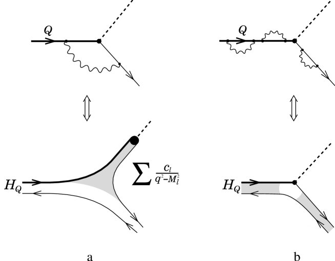
Figure 6: Vertex (a) and external quark leg (b) renormalizations of weak decay amplitudes, and their hadronic counterparts.

This perturbative computation has an exact analogy for the actual meson formfactors. The absence of the vertex corrections means the absence of the $t$-channel resonance contributions at $q_{-}=0$. This fact is directly seen in the explicit expressions for the formfactors in the kinematics where the fraction of the total light-cone momentum $\omega$ corresponding to the momentum transfer $q$, goes to zero. All the strong interaction effects occur in the initial and the final states and are described by using the exact eigenfunctions instead of the plane waves.

At $q_{-}\neq 0$ the vertex corrections appear to order $g_{s}^{2}$, and already the first $g_{s}^{2}$ correction in the coefficient function of the operator $\bar{Q}Q$ becomes different from $(1-\beta^{2}/m_{Q}^{2})^{-1/2}$. The vertex corrections are dual to the $t$-channel resonance contribution in the exact amplitude, and they also appear explicitly with the factors $q_{-}$ and $\beta^{2}$. Additionally, the original tree-level overlap is modified both kinematically and due to the additional terms in the expansion of the $\bar{Q}\gamma_{\mu}q$ current in terms of the light-cone spinors. All this is directly observed in the explicit expressions for the meson transition formfactors.

Regarding the two other assumptions, the fact that the transition formfactors are regular functions of $q^{2}$ can be seen, of course, from their most general analytic expressions. Another way to visualize this is to use the approximate scaling behavior

$$\frac{1}{\sqrt{2m_{Q}}}\,\langle k|J_{\mu}(q)|H_{Q}(m_{Q})\rangle\;\simeq\;\frac{1}{\sqrt{2m_{Q}^{\prime}}}\,\langle k|J_{\mu}(q^{\prime})|H_{Q}(m_{Q}^{\prime})\rangle\;,$$ (76)

where $q^{\prime}$ is adjusted in respect to $m_{Q}^{\prime}$ to have the same rest-frame momentum of the final-state meson $k$:

$${q^{\prime}}^{2}\;=\;\frac{M_{H_{Q}}(m_{Q})}{M_{H_{Q}}(m_{Q}^{\prime})}q^{2}\,+\,M_{H_{Q}}(m_{Q}^{\prime})\left(M_{H_{Q}}(m_{Q}^{\prime})\!-\!M_{H_{Q}}(m_{Q})\right)\,+\,M_{k}^{2}\left(1\!-\!\frac{M_{H_{Q}}(m_{Q})}{M_{H_{Q}}(m_{Q}^{\prime})}\right)\,.$$ (77)

This freedom can be used, say, to make momentum transfer $q$ light-like,

$$m_{Q}^{\prime}\;\simeq\;m_{Q}\;-\;\left[\frac{m_{Q}^{2}-M_{k}^{2}+q^{2}}{2m_{Q}}-\sqrt{\left(\frac{m_{Q}^{2}-M_{k}^{2}-q^{2}}{2m_{Q}}\right)^{2}+\frac{q^{2}M_{k}^{2}}{m_{Q}^{2}}}\;\right]$$ (78)

and then use the exact representation of the amplitudes via the simple wavefunctions overlaps. This trick allows one, for example, to see the strong suppression of the transition amplitudes to highly excited states $M_{k}^{2}\sim m_{Q}^{2}\gg\beta m_{Q}$ at non-zero $q^{2}$ as well, without going into details described in Appendix 2. The relation Eq. (76) is violated by the $\beta^{2n}$ radiative corrections and by the subleading $1/m_{Q}$ terms in the expansion of the current $J_{\mu}$, which are both power suppressed here. It can be derived directly from the explicit solution of the model, see Sects. 2 and 4 of Appendix 2.

6 Comments on the literature

Two recent papers [28, 18] claimed to have established inapplicability of the OPE for the heavy flavor widths considering the solvable ’t Hooft model. Ref. [28] addressed the conventional spectator-independent decay channels. Numerically evaluating the possible two-body decay rates for the values of $m_{Q}$ up to $m_{Q}=14$, it found a small systematic excess of the decay width over the free quark diagram which was fitted as

$$\frac{\Gamma_{H_{Q}}-\Gamma_{Q}}{\Gamma_{Q}}\;\sim\;0.15\frac{\beta}{m_{Q}}\;.$$ (79)

This was regarded as the demonstration of (a priori proclaimed) non-existence of the OPE for the nonleptonic widths. Since in the large-$N_{c}$ limit the difference between the nonleptonic and semileptonic widths disappears, this – if true – would mandate the same absence of the OPE for the semileptonic widths as well, an obvious fact ignored by the authors.

In contrast, Ref. [12] accomplished the analytic summation of the large-$m_{Q}$ width in the ’t Hooft model, and no deviation from the OPE was found to the high enough orders in $1/m_{Q}$ (the exact power addressed depended on the values of the final state masses). In particular, the absence of the $1/m_{Q}$ corrections to the parton result for $m_{u,d}\sim\beta\ll m_{Q}$ was very transparent. Additionally, the correspondence was established between the step-by-step quark-gluon based OPE computations and the matching contributions in the integrals determining the meson formfactors in terms of the ’t Hooft wavefunctions. This allows one to compare the OPE computations to the hadronic saturation at the intermediate stages rather than only for the final result.

What could go wrong with the numerical analysis of Ref. [28]? We note that the apparent “effect” was really small numerically and, in the fiducial range of $m_{Q}/\beta\sim 8\;\mbox{to}\;10$ constituted only about $1\%$. Moreover, a closer look at the plots of Ref. [28] shows that the reported discrepancy somewhat increased toward the upper values of $m_{Q}$. As a result, a better fit of the numerical points of Ref. [28] would be achieved assuming small ${\cal O}(1/m_{Q}^{0})$ (not power-suppressed!) corrections to the width, with the numerical coefficient $\sim{\cal O}(10^{-2})$. Unfortunately, a priori targeting the $1/m_{Q}$ terms, the authors did not explore the possibility of alternative interpretations.

Incidentally, the scale of the claimed discrepancy lies just in the magnitude range of the $1/m_{Q}^{2}$ effects from the OPE which could be a priori expected at $m_{Q}\approx 10$. It turns out that the numerical points for $\Gamma(m_{Q})$ in Ref. [28] can be well fitted by the leading-$m_{Q}$ expression and adjustable $\beta^{2}/m_{Q}^{2}$ terms with the coefficient ${\cal O}(1)$. Adding arbitrary corrections $\sim\beta^{3}/m_{Q}^{3}$ with the larger coefficient up to $6\div 8$ allows really perfect fits. Since the actual $1/m_{Q}^{3}$ corrections include the expectation values of the four-quark operators which are not given by factorization, they are uncertain. Their estimates showed that they are typically significantly enhanced compared to the naive dimensional estimate $\sim\beta$.

Thus, the question would remain open before the actual OPE corrections are computed. This was accomplished in Ref. [12]. While the radiative correction enhances the width by the factor $1+\beta^{2}/(2m_{Q}^{2})$ to order $1/m_{Q}^{2}$, the kinetic term $-\mu_{\pi}^{2}/(2m_{Q}^{2})$ tends to suppress it. Therefore, if, as stated in Ref. [28], the plotted values refer to the bare mass $m_{Q}$, it seems that the numerical calculation reported by Grinstein and Lebed yielded the result exceeding the asymptotic width by an amount ranging from a fraction to a per cent.

The most apparent resolution, in our opinion, is that the analysis of Ref. [28] simply does not control the accuracy of the numerical computations of the amplitudes at the required level of a few per mill. This is not surprising and roots to the well-known problems of numerical computations. The width at large $m_{Q}$ is saturated by highly excited states whose wavefunctions oscillate fast. This standard problem of the numerical computations of the semiclassical transition overlaps is additionally plagued by the general complexity of the numerical solutions of the ’t Hooft equation and the encountered singular integrals. These problems were alluded to in Ref. [28].

The general lesson one draws from this comparison is not new: it is not easy to correctly evaluate the actual asymptotic width in too straightforward numerical summations of many exclusive widths, were it a computer-simulated approximate solution for a theoretical model with – theoretically speaking – potentially unlimited accuracy, or the actual experimental data. The approximations made in practical applications usually go across preserving the subtle interplay of different effects which underlies delicate cancellations shaping the size and scaling of the power suppressed nonperturbative effects.

The recent paper Ref. [18] announced even more drastic numerical mismatch of the actual hadronic width vs. the OPE considering WA, even in the leading order at which the effect appears. In Sects. 3 and 4, on the contrary, we analytically computed the asymptotics of the spectator-dependent widths and found exact correspondence with the OPE. As a matter of fact, Ref. [18] contains self-contradicting assertions: It was stated that the (smeared) current-current vacuum correlator (of the type determining, say, $\sigma({\rm e^{+}e^{-}}\to\mbox{hadrons})$) is known to obey the OPE. Simultaneously, the difference was claimed established for the effect of WA in the context relying on the factorization expression Eq. (27). The starting expression – whether correct or not for a particular model – thus equates the validity of the OPE for the WA nonleptonic width to its applicability for the vacuum current correlator. Fig. 7 shows the ratio of the (smeared) values of the absorptive parts of the correlator,

$$\frac{{\rm Im}\,\Pi_{\mu\mu}(q^{2})}{{\rm Im}\,\Pi_{\mu\mu}^{\rm tree}(q^{2})}$$

according to Ref. [18]. The variance from unity, in general, does seem to be present.

Figure 7: The actual–to–partonic ratio of the absorptive part of the vector current correlator at $m_{u}\!=\!m_{d}\!=\!0.56\beta$, according to Ref. [18], for $N_{c}=10$ (solid line) and $N_{c}=20$ (dashed line). Energy scale is in units of $\beta$. Smearing procedure has been applied for the hadronic cross section.

We do not think that this warrants one to become cautious in applying the OPE to the polarization operator. There are certain drawbacks in the computations of Ref. [18]. For unknown reasons the authors presumed that the width Eq. (27) becomes non-integrable for the large-$N_{c}$ theory and, therefore, cannot be sensibly smeared. As a result, instead of considering the current correlator in the ’t Hooft model itself, a rather ad hoc ansatz was adopted which was intended to mimic nonvanishing widths of the resonances at finite $N_{c}$. The simple resonant representation for $\Pi(q^{2})$,

$$\Pi(q^{2})\;=\;N_{c}\sum_{n}\,\frac{c_{n}^{2}}{q^{2}-M_{n}^{2}+i\epsilon}\;,\qquad-{\rm Im}\,\Pi(q^{2})\;=\;\pi N_{c}\sum_{n}\,c_{n}^{2}\,\delta\left(q^{2}-M_{n}^{2}\right)$$ (80)

was replaced by a complicated model where ${\rm Im}\,\Pi(q^{2})$ was due to the two-meson states, with their production amplitude containing the resonance terms

$$\frac{\sqrt{N_{c}}c_{n}}{q^{2}-M_{n}^{2}+iM_{n}\Gamma_{n}}\;.$$

At large $N_{c}$ the residues $\sqrt{N_{c}}c_{n}\sim\sqrt{N_{c}}$ while the resonance decay amplitudes ${\cal M}_{nkl}\sim 1/\sqrt{N_{c}}$; the widths $\Gamma_{n}\sim 1/N_{c}$.

As soon as $\Gamma_{n}$ are small enough, such a prescription does not differ from the proper spectral density Eq. (80) being a concrete functional choice of the $\delta$-distributions,

$$\int_{|q^{2}-M_{n}^{2}|\gg M_{n}\Gamma_{n}}\;{\rm d}q^{2}\>\frac{c_{n}^{2}}{|q^{2}-M_{n}^{2}+iM_{n}\Gamma_{n}|^{2}}\;=\;\pi\,c_{n}^{2}\,\frac{1}{M_{n}\Gamma_{n}}\;,$$ (81)

provided each $\Gamma_{n}$ is saturated by the included decay modes:

$$\sum_{k,l}|{\cal M}(n\,\to k\,l)|^{2}\cdot\Phi_{kl}\;=\;2\,M_{n}\,\Gamma_{n}\;.$$ (82)

Here $\Phi_{kl}$ denote the two-body decay phase space. Under these constraints such a model – if not true – is at least legitimate. However, two conditions must be observed: First, the resonances do not overlap, $\Gamma_{n}\ll|M_{n\pm 1}\!-\!M_{n}|$. Additionally, the partial decay amplitudes and the phase space factors must be practically constant within the (total) width of the individual meson.

Both constraints are satisfied in the formal limit $N_{c}\to\infty$. However, in practice the width grows with the mass of the resonance, while the spacing between the successive ones decreases. Therefore, for finite $N_{c}$ adopted in Ref. [18] (let alone the considered case $N_{c}=1\,$!) the first condition was not well respected. Regarding the second constraint, the problem gets additionally aggravated by the singular two-body phase space in $D=2$. Therefore, it seems quite probable that the reported disagreement is rooted to the inconsistencies of the model for ${\rm Im}\,\Pi(q^{2})$ adopted in Ref. [18].

A detailed look at the plots displayed there incidentally provides support for this conjecture. The plots for (the smeared) ${\rm Im}\,\Pi(q^{2})$ show a rather unphysical shoulder at $m_{Q}\approx 10$ which coincides with the mass of the resonance having abnormally large width (Fig. 9 of Ref. [18]). On the other hand, the agreement between the hadronic and quark widths is surprisingly good just at lower masses where the resonances are more narrow. The point where the curves start to diverge, apparently shifts upward with increasing $N_{c}$.

Finally, a simpler question remains open about the accuracy of numerical computations employed in Ref. [18]. Taken at face value, even adopted sampling of $m_{Q}$ when only 2 to 3 points fall inside a separate sharp resonance peak, seems insufficient to evaluate the smeared width reliably. Whether these effects can explain the observed discrepancy $\sim 20\%$ at $m_{Q}\sim\;10\mbox{ to }15$, remains to be clarified.

It is worth reiterating that the computational difficulties – quite significant in the analysis of Ref. [18] – to a large extent were a hand-made problem. Both $c_{n}$ and $M_{n}$ are readily computed without cumbersome triple overlaps involving singular integrals, and in any case had been determined to construct the authors’ model. Computing the smeared width directly from Eq. (80) would be then quite straightforward.

7 Conclusions

We have examined the inclusive decay widths of heavy flavor mesons in the ’t Hooft model in the context of the heavy quark expansion, paying attention to the spectator-dependent effects sensitive to the flavor of the spectator quark. To the order the high-energy asymptotics are calculated, there is no deviation from the OPE predictions, either for semileptonic, nonleptonic decays or for the ${\rm e^{+}e^{-}}\to\mbox{hadrons}\,$-type processes – as anticipated.

We confirm that there is no difference for the OPE whether a semileptonic or nonleptonic width is considered. What matters is only whether the particular observable can be represented as the complete discontinuity of the properly constructed correlation function over the cut in a suitable “hard” variable. This variable, $\omega$, is the same for both semileptonic and nonleptonic decays, Eq. (29). After that the only difference is the number of the quark Green functions to be multiplied and to perform the expansion of the product in the complex plane. The validity of the OPE, of course, cannot depend on these technicalities.

This does not mean, however, that for all types of decays the predictions of practical OPE truncated after the first few terms, work with equal accuracy at a fixed mass $m_{Q}$. On the contrary, considerations of Ref. [29] suggest that the effective “hardness” scale can be smaller than literally the energy release. Accordingly, higher onset of duality and larger deviations for nonleptonic widths were obtained in Ref. [13] in the instanton-based model.

Therefore, in our opinion, attempts to check (let alone to disprove) the OPE itself in the concrete model are hardly meaningful beyond illustrative purposes. What has a potential of providing useful insights, is studying the behavior of the contributions violating local duality, so far the least understood theoretically subject.

The “practical” OPE yields the width in the power expansion

$$\frac{\Gamma_{H_{Q}}}{\Gamma_{0}}\;=\;A_{0}+\frac{A_{1}}{m_{Q}}+\frac{A_{2}}{m_{Q}^{2}}\>+\;...\;\;.$$ (83)

If the series in $1/m_{Q}$ were convergent (to the actual ratio), $\Gamma_{H_{Q}}$ would have been an analytic function of $m_{Q}$ above a certain mass $m_{0}$ pointing to the onset of the exact local parton-hadron duality. The actual $\Gamma_{H_{Q}}$ is definitely non-analytic at any threshold (whether or not the amplitude vanishes at the threshold). Thus, the ‘radius of convergence’ cannot correspond to the mass smaller than the threshold mass. Since in the actual QCD the thresholds exist at arbitrary high energy, the power expansion in Eq. (83) can be only asymptotic, with formally zero radius of convergence in $1/m_{Q}$.

In practice, the true threshold singularities are expected to be strongly suppressed at large energies, and the corresponding uncertainties in the OPE series quite small. In actual QCD they are expected to be exponentially suppressed eventually, though, possibly, starting at larger energies. In the intermediate domain they can decrease as a certain power and must oscillate.

As was illustrated in Ref. [12], the power expansions like Eq. (83) are meaningful even beyond the power suppression where the duality-violating oscillations show up. In the case of the heavy quark widths where mass $m_{Q}$ cannot be varied in experiment, the size of the duality-violating component may set the practical bound for calculating the widths. Thus, it is important to have an idea about its size. We emphasize that one should always include the leading QCD effects to the partonic expressions, rather than compare the actual observable with the bare quark result. In the model considered in Ref. [12], incorporating the power corrections from the practical OPE suppressed the apparent deviations by more than an order of magnitude.

It is worth noting that we identified the case where the exact quark-hadron duality in the interference width is saturated on a single final state. It is realized in the chiral limit for the final state quarks. It seems to be just an opposite case to the classical Small Velocity limit for semileptonic decays noted by Shifman and Voloshin in 1986 [8]. While applicable only for large $N_{c}$ and in $D=2$, the present case is peculiar in that the duality is not affected by subleading power corrections. Both cases serve as a counter-example to the lore often purportingly equating the accuracy of local duality to the proliferation of the final state channels in the process in question.

The performed analysis elucidates how the general duality between the partonic and hadronic widths works out its way at large energies. It can be traced that, to the leading order in $1/m_{Q}$, the duality is simply the completeness of eigenstates of the hadronic Hamiltonian. It is not even required to explicitly solve the ’t Hooft equation to establish the leading free quark result for the width, but just to know that the solutions form a complete basis. The absence of the non-OPE terms already at the next to leading order $1/m_{Q}$ is a dynamical fact requiring, for example, a proper solution of the bound-state equations. This enters via the average of the moments of the invariant hadronic mass in the final state.

The ’t Hooft model gives an explicit example of the duality-violating effects, at least of the “minimal”, resonance-related nature. As a general feature, we observe that
— the duality between the appropriately averaged (to eliminate the threshold singularities) hadronic widths and the truncated OPE predictions sets in numerically well rather early, after only a couple of the principal thresholds;
— the local duality works much better in the heavy quark widths, nonleptonic and semileptonic than in $\sigma({\rm e^{+}e^{-}}\to\mbox{hadrons})$. This applies to both the qualitative behavior (generally, a larger density of resonances implying a more narrow minimal interval of smearing) and to the strength of the threshold singularities as well as the threshold residues. The qualitative discussion of the underlying reason can be found in Ref. [30], Sect. 3.5.3.

Can these lessons be transferred to actual QCD? Unfortunately, there are some essential differences between it and the explored ’t Hooft model, which must be important for the local duality violation.

The singular $1/|\vec{p}\,|$ two-body phase space in $D=2$ strongly enhances the threshold singularities, compared to $|\vec{p}\,|$ in $D=4$. In the actual QCD enhancement of the non-smooth behavior can rather be expected only from single resonances with masses close to $M_{B}$. While infinitely narrow at $N_{c}\to\infty$, they acquire significant width for $n_{f}/N_{c}$=1 which leads to drastic flattening of the resonance-related combs when the width becomes comparable to the distance between the successive resonances. Additionally, one expects a denser resonance structure, at least asymptotically, in the actual QCD in four dimensions (even at $N_{c}\to\infty$) than the equal in $M^{2}$ spacing in $D=2$. All this would lead to suppression of the duality violation.

Finally, similar types of the condensate corrections lead to a weaker suppression in $D=2$ due to the smaller dimension of the corresponding operators. This provides a larger room for various possible nonperturbative effects.

These obvious differences would optimistically suggest that the ’t Hooft model represents, in a sense, an upper bound for violations of local duality in QCD. While this is not excluded, such implications must be regarded with caution.

In fact, the largest duality violating effects in the nonleptonic heavy flavor decays can be expected from the resonance structures in the combined $(\bar{q}q\bar{q}q)$ channel in the final state, embedding the quarks belonging to both the “semileptonic” and “hadronic” subprocesses which do not decouple completely. Such states are lost in the ’t Hooft model. Moreover, the limit $N_{c}\to\infty$ simply erases the difference between the nonleptonic and semileptonic decays in this respect.

Another peculiarity of QCD in two dimensions is absence of the real gluonic degrees of freedom and of the perturbative logarithmic short-distance corrections typical for $D\!=\!4$ (in contrast to the power-like ones in the super-renormalizable $D\!=\!2$ QCD). So far we have no clues if the onset of duality for excitation of the gluonic degrees of freedom is the same or noticeably larger than for the processes describing the evolution of the “valence” quarks. Correspondingly, while observing a good qualitative duality between the bare quark computations and the actual hadronic probabilities already at energies $\sim 1\,\mbox{GeV}$, one may have to ascend to higher energies in the Minkowski domain to reach quantitative agreement at the level of the perturbative corrections. Let us note in this respect that the ‘real gluons’ in jet physics are reliably observed in experiment only at rather high energies. Unfortunately, two-dimensional theories do not allow one to study this interesting aspect of local gluon-hadron duality even in the accessible model settings.

As emphasized above, we found that the OPE predictions universally hold for the inclusive widths. In this respect, the origin of the paradox in mismatch between the size of the interference term on the quark and meson languages, Eqs. (2) and (4), is quite transparent. The mismatch emerges in the $N_{c}$-suppressed term. Addressing such effects requires a more accurate control of decay amplitudes beyond the leading-$N_{c}$ counting rules. In particular, it is necessary to account for $1/N_{c}$ corrections in the color-allowed amplitudes rather than use oversimplified prescription like Eq. (3) (a possible resolution was conjectured already in Ref. [17]).

A closer look reveals that the problem originates just on the quark configurations where all four quarks in the intermediate state have the same color. This configuration is $1/N_{c}$ suppressed and can be simply discarded for the leading-$N_{c}$ probabilities. Within this color combination, there is an ambiguity of allocating the quarks over the colorless mesons which is absent otherwise. It is not difficult to see that the naive computations based on the amplitude prescription Eq. (3) amounts to counting the two possibilities independently, which is not justified a priori. Moreover, it is a clear double counting at least in the simple quark picture. To phrase it differently, the bases of the final states used in the naive color rules like Eq. (3), are non-orthogonal beyond the leading order in $N_{c}$.

With the complicated confinement dynamics, we cannot know beforehand what are the actual decay amplitudes to the particular hadronic states in this case – and, additionally, the simple two-meson picture of the final state must be, in general, extended when going beyond the leading order in $N_{c}$. However, it seems obvious that the naive prescription have little chance to be true in a complete theory if it violates general requirements even in the simplest case of almost free constituents.

This, incidentally, is an illustration of the fact that the naive factorization of decay amplitudes must be violated at some point at the $1/N_{c}$ level – either in the corrections to the color-allowed amplitudes, or at the leading level for color-suppressed amplitudes, or in both. A dedicated study of the above inconsistency was undertaken in the framework of the nonrelativistic quark model in Ref. [31]. It was found that the problem is indeed resolved there in this way, with the concrete dynamical mechanism dominating the modification of the $1/N_{c}$-suppressed amplitudes depending on details of the model.

In Sect. 4, considering the spectator-dependent preasymptotic correction we formulated the problem of calculating the interference width in the way that allowed us to avoid the complications associated with the analysis of the $N_{c}$-subleading transition amplitudes, and to study it in the theoretically clean environment. Incorporating the spectator quark via PI made interference an effect appearing in the same order in $N_{c}$ as the non-interference widths. Then the hadron-based computation could be performed consistently, and the OPE prediction was readily reproduced.

Acknowledgments:   N.U. would like to thank V. Petrov for interesting discussions. We are deeply grateful to our collaborators M. Shifman and A. Vainshtein for their generosity in sharing their insights with us and for critical comments on the manuscript. N.U. is grateful to M. Burkardt for useful discussions and to R. Lebed for a number of clarifications and for pointing out some omissions in the original text. This work was supported in part by the National Science Foundation under the grant number PHY 96-05080 and by the RFFI under the grant number 96-15-96764.

Appendices

A1 ’t Hooft wavefunctions in the semiclassical regime and the UV divergences

Here we outline a more accurate determination of the scaling with $\Lambda$ of the smearing parameter $\Delta$ in Eqs. (41)-(44).

At $M_{n}\gg\beta,\>m_{u,d}$ the solutions of the ’t Hooft equations are nearly free and approach the massless solutions [19, 32]

$$\varphi_{n}(x)\;\simeq\;\sqrt{2}\cos{\pi nx}\;,\qquad M_{n}^{2}\,\approx\,\pi^{2}\beta^{2}n\;.$$ (A1.1)

The first expression holds outside the end-point domains $x\to 0$ and $x\to 1$ bounded by the “classical turning points”

$$x,\;1-x\;\simeq\frac{m^{2},\beta^{2}}{M_{n}^{2}}\;.$$ (A1.2)

We again imply the simplified case of equal quark masses $m_{u}=m_{d}=m$. The semiclassical wavefunctions (A1.1) determine the ultraviolet-singular part of the Green functions.

We shall adopt the exponential regularization of the sums. Then the Green function $G(x,y;\Lambda)$ in Eq. (41) has a meaning of the Euclidean Green function for the ’t Hooft light-cone Hamiltonian, with $1/\Lambda^{2}$ corresponding to the Euclidean (imaginary) light-cone “time” $ix_{+}$, and $x,y$ being “coordinates” in the space of the light-cone momentum fractions. Formally, the problem is equivalent to usual one-dimensional quantum mechanics on the interval $[0,1]$ with Hamiltonian given by the r.h.s. of Eq. (19). The first (local) terms play a role of the potential whereas the integral term includes the counterpart of the kinetic energy which is now approximately $\pi|k|$ for the “momentum” $k$ much larger than $\beta$.

The regularized summation is straightforward and yields literally for $G(x,y;\Lambda)$

$$\frac{1}{4}\,\frac{\sinh{\epsilon}}{\sinh^{2}{\frac{\epsilon}{2}}+\sin^{2}{\frac{\pi}{2}(x-y)}}\;+\;\frac{1}{4}\,\frac{\sinh{\epsilon}}{\sinh^{2}{\frac{\epsilon}{2}}+\sin^{2}{\frac{\pi}{2}(x+y)}}\;,\qquad\epsilon\equiv\frac{\pi^{2}\beta^{2}}{\Lambda^{2}}\;.$$ (A1.3)

Since the small-$n$ eigenfunctions can be quite different from Eq. (A1.1), there can be, a priori, additional regular ($\epsilon$-independent) terms in Eq. (A1.3). However, since at $\epsilon\to 0$ the limit of $G$ must yield $\delta$-function, they are absent.

The first term in Eq. (A1.3) clearly yields $\delta(x-y)$ at $\epsilon\to 0$:

$$\frac{1}{4}\,\frac{\sinh{\epsilon}}{\sinh^{2}{\frac{\epsilon}{2}}+\sin^{2}{\frac{\pi}{2}(x-y)}}\;\approx\;\frac{\epsilon}{\epsilon^{2}+\pi^{2}(x-y)^{2}}\;,$$ (A1.4)

with the width $\Delta$ at finite $\epsilon$ amounting to

$$\Delta\;=\;\frac{\epsilon}{\pi}\;=\;\frac{\pi\beta^{2}}{\Lambda^{2}}\;.$$ (A1.5)

The second term in Eq. (A1.3) seems to appear when both $x$ and $y$ are small, $x,y\,\mathrel{\hbox to0.0pt{\lower 3.0pt\hbox{\hskip 0.0pt$\sim$}\hss}\raise 1.0pt\hbox{$<$}}\epsilon$ or $1-x,1-y\,\mathrel{\hbox to0.0pt{\lower 3.0pt\hbox{\hskip 0.0pt$\sim$}\hss}\raise 1.0pt\hbox{$<$}}\epsilon$. In this domain, however, wavefunctions $\varphi_{n}(x)$ with $n\mathrel{\hbox to0.0pt{\lower 3.0pt\hbox{\hskip 0.0pt$\sim$}\hss}\raise 1.0pt\hbox{$<$}}\Lambda^{2}$ are different (suppressed), and in reality this term must be discarded. In practice the domain of such small $x$ must be treated separately, which is illustrated below. Therefore, we adopt

$$G(x,y;\Lambda)\;\simeq\;\frac{1}{4}\frac{\sinh{\epsilon}}{\sinh^{2}{\frac{\epsilon}{2}}+\sin^{2}{\frac{\pi}{2}(x-y)}}\;\qquad\mbox{ at }\;\frac{1}{\Lambda^{2}}\,\mathrel{\hbox to0.0pt{\lower 3.0pt\hbox{\hskip 0.0pt$\sim$}\hss}\raise 1.0pt\hbox{$<$}}x,y\,\mathrel{\hbox to0.0pt{\lower 3.0pt\hbox{\hskip 0.0pt$\sim$}\hss}\raise 1.0pt\hbox{$<$}}1-\frac{1}{\Lambda^{2}}\;.$$ (A1.6)

To address the end-point domains $x$ or $(1-x)\sim 1/\Lambda^{2}$ we need to account for the corresponding behavior of $\varphi_{n}(x)$ in the “classically forbidden” domain, using the language of ordinary Quantum Mechanics. In these domains the wavefunctions are suppressed:

$$\varphi_{n}(x)\;\sim\;\mbox{const }\left\{\begin{array}[]{ll}\left(\frac{x}{x_{t}}\right)^{\gamma_{1}}&x\mathrel{\hbox to0.0pt{\lower 3.0pt\hbox{\hskip 0.0pt$\sim$}\hss}\raise 1.0pt\hbox{$<$}}x_{t}\ll 1\\ \\ \left(\frac{1-x}{1-x_{t}}\right)^{\gamma_{2}}&1-x\mathrel{\hbox to0.0pt{\lower 3.0pt\hbox{\hskip 0.0pt$\sim$}\hss}\raise 1.0pt\hbox{$<$}}1-x_{t}\ll 1\end{array}\right.\qquad x_{t}\approx\frac{m^{2},\beta^{2}}{\Lambda^{2}}\;.$$ (A1.7)

Now we consider the regularized sum rule Eq. (43):

$$I_{1}(\Lambda^{2})\;=\;\int_{0}^{\infty}\,q^{2}{\rm d}q^{2}\>{\rm e}\,^{-q^{2}/\Lambda^{2}}\,\rho(q^{2})\;=\;\int_{0}^{1}{\rm d}x\,{\rm d}y\;\left(\frac{m^{2}}{x}+\frac{m^{2}}{1-x}\right)\,G(x,y;\Lambda)\;.$$ (A1.8)

Using $G(x,y;\Lambda)$ in the form Eq. (A1.6) we get

$$I_{1}(\Lambda^{2})\;=\;2\cdot m^{2}\left[\ln{\frac{\Lambda^{2}}{\pi\beta^{2}}}\;+\;\mbox{const}\,\right]\;,$$ (A1.9)

where the factor $2$ reflects the contributions of both $x\to 0$ and $x\to 1$. The logarithm is saturated at

$$|x-y|\mathrel{\hbox to0.0pt{\lower 3.0pt\hbox{\hskip 0.0pt$\sim$}\hss}\raise 1.0pt\hbox{$<$}}\frac{\beta^{2}}{\Lambda^{2}}\>,\qquad\frac{\beta^{2}}{\Lambda^{2}}\ll x\ll 1$$ (A1.10)

(and likewise with $x\to 1-x$, $\,y\to 1-y$). In this domain the expression for $G(x,y;\Lambda)$ is legitimate.

Now we show directly that the domain $x\mathrel{\hbox to0.0pt{\lower 3.0pt\hbox{\hskip 0.0pt$\sim$}\hss}\raise 1.0pt\hbox{$<$}}\beta^{2}/\Lambda^{2}$ yields only a constant, that is, a nonsingular contribution at $\Lambda\to\infty$. First, we note that Eq. (38) ensures an upper bound on $c_{n}$, const$/M_{n}^{2}$. More precisely,

$$|c_{n}|\;\leq\;\mbox{const}\cdot\frac{m^{2}}{\gamma}\cdot\frac{1}{M_{n}^{2}}\;\propto\;\frac{1}{n}\;.$$ (A1.11)

This, of course, follows also from Eqs. (44, 45). Then we can bound from above the small-$x$ contribution as

$$\left|\int_{x\mathrel{\hbox to0.0pt{\lower 3.0pt\hbox{\hskip 0.0pt$\sim$}\hss}\raise 1.0pt\hbox{$<$}}\frac{1}{\Lambda^{2}}}{\rm d}x\,{\rm d}y\,\left(\frac{m^{2}}{x}\!+\!\frac{m^{2}}{1\!-\!x}\right)G(x,y:\Lambda)\right|\,\leq\,\mbox{const}\>\frac{m^{2}}{\gamma}\sum_{n=1}^{\infty}\frac{{\rm e}\,^{-\frac{\pi^{2}\beta^{2}n}{\Lambda^{2}}}}{n}\int_{0}^{\Lambda^{-2}}\!{\rm d}x\>\frac{m^{2}}{x}\left(\pi^{2}nx\right)^{\gamma}$$

$$\leq\;\mbox{const}\>\frac{m^{4}}{\gamma^{2}}\,\sum_{n=1}^{\infty}\frac{{\rm e}\,^{-\pi^{2}\beta^{2}n/\Lambda^{2}}}{n}\left(\frac{n}{\Lambda^{2}}\right)^{\gamma}\;\simeq\;\mbox{const}\>\frac{m^{4}}{\gamma^{3}\beta^{2}}\;.$$ (A1.12)

Here we assumed the cutoff in the integral over $x$ at $\sim 1/\Lambda^{2}$, up to an arbitrary constant. The dimensionful factor can be either $\beta^{2}$ or $m^{2}$, whichever is larger and determines the position of the “classical turning” point. The key property is the convergence of both the integral over small $x$ and the sum over $n$ due to the suppression of $\varphi_{n}(x)$ in the “classically forbidden” domain.

Thus, the translation rule for the cutoff energy into the regularization Eq. (42) in the integral over $x,y$ is obtained directly from the ’t Hooft equation.

Using the similar technique, it is easy to establish the asymptotic duality directly for the pseudoscalar current correlator

$$\Pi_{\!{}_{P}}(q^{2})\;=\;N_{c}\,\sum_{n}\>\frac{d_{n}^{2}}{M_{n}^{2}-q^{2}}\;,\qquad\;\frac{1}{\pi}\,\mbox{Im}\>\Pi_{\!{}_{P}}(q^{2})\;=\;N_{c}\,\sum_{n}\>d_{n}^{2}\,\delta(M_{n}^{2}\!-\!q^{2})\;,$$ (A1.13)

where

$$d_{n}\!=\sqrt{\frac{\pi}{N_{c}}}\;\langle n|\bar{d}i\gamma_{5}u|0\rangle\!\!\! = \;\qquad\frac{1}{2}\,\int_{0}^{1}{\rm d}x\left(\frac{m_{d}}{x}\!+\!\frac{m_{u}}{1\!-\!x}\right)\varphi_{n}(x)$$

$$= \!\!\!\frac{1}{m_{u}\!+\!m_{d}}\int_{0}^{1}{\rm d}x\left(\frac{m_{d}^{2}}{x}\!+\!\frac{m_{u}^{2}}{1\!-\!x}\right)\varphi_{n}(x)\;\,\mbox{ (even $n$; $0$ for odd $n$).}$$

(The first form is a direct representation, whereas the second expresses the pseudoscalar density as the divergence of the axial current. A certain parity relation [20] ascending to ’t Hooft ensures they both hold.) To find the asymptotics of $d_{n}$ we consider the logarithmically divergent sum

$$\int{\rm d}q^{2}\,\frac{\rho_{\!{}_{P}}(q^{2})}{q^{2}}\;\propto\;\sum_{n}\,\frac{d_{n}^{2}}{M_{n}^{2}}\;=$$

$$=\;\sum_{n}\,\frac{1}{2(m_{u}\!+\!m_{d})M_{n}^{2}}\,\int_{0}^{1}\!{\rm d}x\left(\frac{m_{d}}{x}\!+\!\frac{m_{u}}{1\!-\!x}\right)\varphi_{n}(x)\>\int_{0}^{1}\!{\rm d}y\left(\frac{m_{d}^{2}}{y}\!+\!\frac{m_{u}^{2}}{1\!-\!y}\right)\varphi_{n}(y)\>.$$ (A1.15)

Eq. (38) allows one to rewrite it as

$$\sum_{n}\frac{d_{n}^{2}}{M_{n}^{2}}=\frac{1}{2(m_{u}\!+\!m_{d})}\,\sum_{n}\,\int_{0}^{1}\!{\rm d}x\left(\frac{m_{d}}{x}\!+\!\frac{m_{u}}{1\!-\!x}\right)\varphi_{n}(x)\,\int_{0}^{1}\!{\rm d}y\,\varphi_{n}(y)\;,$$ (A1.16)

which returns us to Eq. (39).

A2 $1/m_{Q}$ expansion of the heavy quark weak decay amplitudes

As discussed in Sect. 5, the perturbative corrections to the weak decay vertex appear to order $\beta^{2}$. In the light-front formalism they vanish at the kinematic point $q^{2}=0$ [12], since it can be realized as the configuration with $q_{-}=0$, for which no physical states in the $t$ channel is possible. The loop corrections proportional to the dimensionful coupling $\beta^{2}$ can be, therefore, inversely proportional to $m_{Q}^{2}$ or $E_{\rm rel}^{2}\sim(m_{Q}-m_{q}-\sqrt{q^{2}})^{2}$. Since at $m_{Q}-m_{q}-\sqrt{q^{2}}\sim\beta$ the process is ‘soft’, we do not consider here this domain, and do not distinguish between the scales of $m_{Q}$ and $E_{\rm rel}$. It is important that no dynamic gluon degrees of freedom exist in $D=2$. Therefore, in the ’t Hooft model vertex corrections separately are perturbatively infrared finite in physical gauges. This was explicitly illustrated in Ref. [12].

As a result, the actual transition amplitudes $\langle k|J|H_{Q}\rangle$ up to terms $\beta^{2}/m_{Q}^{2}$ must be given by only some overlaps of the initial and final state wavefunctions, at arbitrary (though not too close to $(m_{Q}-m_{q})^{2}$) values of $q^{2}$. We assume that the initial state $H_{Q}$ is either a ground state or has a finite (not scaling with $m_{Q}$) excitation number. The final state $k$ can be arbitrary. We will show that the explicit expressions for the transition amplitudes in the ’t Hooft model exhibit this parton-deduced property.

Let us consider, for example, the representation used in Ref. [28], although we put it in a slightly modified form similar to that of Refs. [33, 23]. One introduces the kinematic variable $\omega$ which depends on $q^{2}$ and the final state meson mass:

$$\omega\;=\;\frac{1}{2}\,\left[1\;+\;\frac{q^{2}-M_{k}^{2}}{M_{H_{Q}}^{2}}\;-\;\sqrt{1-2\frac{q^{2}+M_{k}^{2}}{M_{H_{Q}}^{2}}+\left(\frac{q^{2}-M_{k}^{2}}{M_{H_{Q}}^{2}}\right)^{2}}\;\right]\;,$$ (A2.1)

which, in the light-cone formalism has a meaning of the fraction of the momentum seen in the infinite-momentum frame carried by the particle with mass $\sqrt{q^{2}}$ in the two body decay of $B$ meson, if another particle has mass $M_{k}$. This fraction has two possible values corresponding to the two possible directions of meson $k$ in the rest frame. We chose the above branch to have $q_{-}\to 0$ as $q^{2}\to 0$, as in Ref. [12]. The light-cone fraction $\omega$ has a very simple meaning in the rest frame as well:

$$(1\!-\!\omega)M_{H_{Q}}\;=\;(|\vec{p}_{k}|+E_{k})_{\rm c.m.}\;,\qquad\;\omega M_{H_{Q}}=(-|\vec{q}\,|+q_{0})_{\rm c.m.}\;.$$ (A2.2)

Two $\omega$-dependent $H_{Q}\,D^{(k)}$ overlaps are then considered,

$${\cal C}_{k}(\omega)\;=\;-\frac{1\!-\!\omega}{\omega}\,\int_{0}^{1}\,{\rm d}y\;\varphi_{k}(y)\varphi_{H_{Q}}(\,1-(1\!-\!\omega)(1-y)\,)\;,$$

$${\cal D}_{k}(\omega)\;=\;-\omega\,\int_{0}^{1}\,{\rm d}y\;\frac{\varphi_{k}(y)}{y}\frac{\varphi_{H_{Q}}(\,1-(1\!-\!\omega)(1-y)\,)}{1-(1\!-\!\omega)(1-y)}$$ (A2.3)

which correspond to the effects unrelated to vertex corrections.

Additionally, in the $t$ channel of the decay process one can have various bound states of $B_{c}$ mesons; we reserve index $l$ for them, and their masses will be denoted $\mu_{l}$. For each $t$-channel resonance there is an $\omega$-dependent triple-meson (“$H_{Q}B_{c}^{(l)}D^{(k)}$”) overlap

$$F_{lk}(\omega)=\omega(1\!-\!\omega)\int_{0}^{1}\!{\rm d}x\int_{0}^{1}\!{\rm d}y\frac{\varphi_{l}^{B_{c}}(x)\varphi_{k}(y)}{[\omega(1\!-\!x)\!+\!(1\!-\!\omega)y]^{2}}\>\left\{\varphi_{H_{\!Q}}(\omega x)\!-\!\varphi_{H_{\!Q}}(1\!-\!(1\!-\!\omega)(1\!-\!y))\right\}\!.$$ (A2.4)

With these notations one has for the transition amplitudes

$$\epsilon_{\mu\nu}q_{\mu}\,\langle k|\,\bar{q}\gamma_{\nu}Q\,|H_{Q}(P)\rangle=\frac{\beta^{2}\sqrt{\pi}}{\sqrt{N_{c}}}\sum_{l}\frac{q^{2}+(-1)^{l}\mu_{l}^{2}}{q^{2}-\mu_{l}^{2}}\,f_{l}F_{lk}(\omega)\>-\,q^{2}{\cal C}_{k}(\omega)\,+\,m_{Q}m_{q}{\cal D}_{k}(\omega)\,,$$

$$q_{\mu}\,\langle k|\,\bar{q}\gamma_{\mu}Q\,|H_{Q}(P)\rangle=\frac{\beta^{2}\sqrt{\pi}}{\sqrt{N_{c}}}\sum_{l}\frac{-q^{2}\!+\!(\!-1\!)^{l}\mu_{l}^{2}}{q^{2}-\mu_{l}^{2}}\,f_{l}F_{lk}(\omega)\>+\,q^{2}{\cal C}_{k}(\omega)\,+\,m_{Q}m_{q}{\cal D}_{k}(\omega)\,.$$

Here, for convenience, we wrote the invariant combinations of the amplitudes instead of the two Lorentz components of the current separately. For example, the decay amplitude $B\rightarrow D^{(k)}+\pi^{(n)}$ in the considered case of vector-like interactions takes the form

$${\cal M}_{kn}\;=\;\frac{G}{\sqrt{2\pi}}\>c_{n}\,\left[\sum_{l}\frac{-P_{n}q^{2}+(-1)^{l}\mu_{l}^{2}}{q^{2}-\mu_{l}^{2}}\,c_{l}F_{lk}(\omega)\;+\;P_{n}q^{2}{\cal C}_{k}(\omega)\;+\;m_{Q}m_{q}{\cal D}_{k}(\omega)\>\right]\;,$$ (A2.5)

where $P_{n}$ is the parity $(-1)^{n+1}$ of the $\pi^{(n)}$ state. Here and below throughout this Appendix we suppressed the factors $N_{c}$ and put dimensionful $\beta=1$. It is easy to see that at $q^{2}=0$ ($\omega\to 0$) only the term $\sim{\cal C}_{k}$ survives and this expression indeed reduces to Eqs. (56, 62).

We shall show that the first term in this relation associated with the dynamics in the $t$ channel, is $1/m_{Q}^{2}$-suppressed compared to the terms given by overlaps ${\cal C}$ and ${\cal D}$. This implements the approximate “on-shell” condition for the heavy quark $Q$; in this case it can be accomplished employing the $1/m_{Q}$ expansion of the initial-state wavefunction $\varphi_{H_{Q}}$.

A2.1 Nonrelativistic expansion in the ’t Hooft equation

To analyze the heavy quark system, it is advantageous to introduce the nonrelativistic variables:

$$M_{n}\;=\;m_{Q}\,+\,\epsilon_{n}\;,\qquad t\,=\,(1-x)m_{Q}\qquad\mbox{and}\qquad\Psi_{n}(t)\,=\,\frac{1}{\sqrt{m_{Q}}}\>\varphi_{n}\left(1-\frac{t}{m_{Q}}\right)\;,$$ (A2.6)

in terms of which the equation takes the form

$$\left(\epsilon_{n}\!+\!\frac{\epsilon_{n}^{2}\!+\!1}{2m_{Q}}\right)\Psi_{n}(t)\;=\;\left(\frac{m_{\rm sp}^{2}\!-\!1}{2t}+\frac{t}{2}\frac{1\!-\!\frac{1}{m_{Q}^{2}}}{1\!-\!\frac{t}{m_{Q}}}\right)\Psi_{n}(t)\;-\;\frac{1}{2}\,\int_{0}^{m_{Q}}{\rm d}s\>\frac{\Psi_{n}(s)}{(t-s)^{2}}\;\;.$$ (A2.7)

The asymptotics of $\Psi_{n}(t)$ at $1\ll t\ll m_{Q}$ is given by

$$\Psi_{n}(t)\;\simeq\;\frac{F_{n}}{t^{3}}\qquad\mbox{with}\qquad F_{n}\;=\;\sqrt{\pi m_{Q}}\,f_{n}\;=\;\int_{0}^{m_{Q}}\,dt\;\Psi_{n}(t)\;\;.$$ (A2.8)

One can extend the bound-state problem Eq. (A2.7) from $[0,m_{Q}]$ to the whole interval $[0,\infty)$ if the exact linear potential term $\frac{t}{2}\left((1-1/m_{Q}^{2})/(1-t/m_{Q})\right)$ is replaced by its formal expansion in $t/m_{Q}$. This is justified literally only up to $1/m_{Q}^{4}$ terms ($1/m_{Q}^{3}$ in the wavefunction), when the ultraviolet divergences of the static heavy quark expansion first show up. Further terms can be obtained using the explicit large-$t$ asymptotics in Eq. (A2.8) and the end-point behavior of $\Psi_{n}(t)$ at $t\to m_{Q}$. For example, the improved nonrelativistic equation takes the form

$$\left(\epsilon_{n}\!+\!\frac{\epsilon_{n}^{2}\!+\!1}{2m_{Q}}\right)\Psi_{n}(t)\,=\,\frac{m_{\rm sp}^{2}\!-\!1}{2t}\,\Psi_{n}(t)+\frac{1}{2}\left[\left(1\!-\!\frac{1}{m_{Q}^{2}}\right)t+\left(1\!-\!\frac{1}{m_{Q}^{2}}\right)\frac{t^{2}}{m_{Q}}+\frac{t^{3}}{m_{Q}^{2}}\right]\,\Psi_{n}(t)$$

$$-\;\frac{1}{2}\,\int_{0}^{\infty}\;{\rm d}s\,\Psi_{n}(s)\,\frac{1}{(t-s)^{2}}\;\;.$$ (A2.9)

Eq. (A2.9) can be viewed as a usual variational problem for the non-local Hamiltonian defined as

$$\langle\Psi|{\cal H}|\Psi^{\prime}\rangle\,=\,\int_{0}^{\infty}\!{\rm d}t\,\Psi(t)\left[\frac{m_{\rm sp}^{2}\!-\!1}{2t}+\frac{1}{2}\left(1\!-\!\frac{1}{m_{Q}^{2}}\right)t+\left(1\!-\!\frac{1}{m_{Q}^{2}}\right)\frac{t^{2}}{2m_{Q}}+\frac{t^{3}}{2m_{Q}^{2}}\right]\,\Psi^{\prime}(t)$$

$$-\;\frac{1}{2}\,\int_{0}^{\infty}\;{\rm d}t\,\int_{0}^{\infty}\;ds\frac{\Psi(t)\Psi^{\prime}(s)}{(s-t)^{2}}\;\;.$$ (A2.10)

For example, the analogue of the nonrelativistic expansion for the heavy hadron mass takes the form

$$M_{H_{Q}}\!-\!m_{Q}\,=\,\langle t\rangle-\frac{1}{2m_{Q}}+\frac{3\langle t^{2}\rangle\!-\!\langle t\rangle^{2}}{2m_{Q}}+\frac{4\langle t^{3}\rangle\!-\!3\langle t\rangle\langle t^{2}\rangle\!+\!\langle t\rangle^{3}}{2m_{Q}^{2}}-\frac{\langle t\rangle}{2m_{Q}^{2}}\,+\,{\cal O}\!\left(\frac{1}{m_{Q}^{3}}\right)\,,$$ (A2.11)

with the average $\langle...\rangle$ defined in the standard way as the integral over $t$ with the weight $|\Psi(t)|^{2}$. Here all averages are calculated with the finite-$m_{Q}$ $\Psi(t)$. To exclude the Coulomb interaction term we used certain relations which are derived in the way analogous to the virial theorem in Quantum Mechanics. Namely, for any eigenfunction $\Psi_{n}(t)$ we can consider the average of ${\cal H}$ over the trial function $\sqrt{\lambda}\,\Psi_{n}(\lambda t)$, and require a minimum at $\lambda=1$ (a similar trick was used in Ref. [24] for the case of infinite $m_{Q}$). In this way one obtains

$$(m_{\rm sp}^{2}-1)\langle\frac{1}{t}\rangle\;-\;\langle{\cal V}\rangle\;-\;\left(1-\frac{1}{m_{Q}^{2}}\right)\langle t\rangle\;-\;2\,\frac{\langle t^{2}\rangle}{m_{Q}}\;-\;3\,\frac{\langle t^{3}\rangle}{m_{Q}^{2}}\;=\;{\cal O}\left(\frac{1}{m_{Q}^{3}}\right)$$ (A2.12)

while

$$\epsilon_{n}+\frac{\epsilon_{n}^{2}+1}{2m_{Q}}=\frac{1}{2}\left((m_{\rm sp}^{2}-1)\langle\frac{1}{t}\rangle-\langle{\cal V}\rangle\right)+\frac{1}{2}\left(1-\frac{1}{m_{Q}^{2}}\right)\langle t\rangle+\frac{1}{2}\frac{\langle t^{2}\rangle}{m_{Q}}+\frac{1}{2}\frac{\langle t^{3}\rangle}{m_{Q}^{2}}\;+\;{\cal O}\left(\frac{1}{m_{Q}^{3}}\right),$$ (A2.13)

where $\langle{\cal V}\rangle$ denotes the expectation value of the integral term in the equation.

The bound-state–independent term $-1/2m_{Q}$ in Eq. (A2.11) deserves a special note: it represents the short-distance renormalization of the bare mass we used, originating from momenta $\sim m_{Q}$. There is no infrared part of the mass: it enters at the scale much larger than $\Lambda_{\rm QCD}$. The effect of smaller momenta is described by the nonperturbative ’t Hooft wavefunction rather than infrared-divergent perturbative diagram.

Let us note that the operator $t/2$ is associated with the breaking of scale-invariance of the static ’t Hooft equation (i.e. $\Psi(\lambda t)$ is the solution of the equation with the linear term $\lambda^{2}t/2$). In other words, the commutation relation holds $\Big{[}t\frac{\rm d}{{\rm d}t},{\cal H}_{\infty}\Big{]}\!=\!t\!-\!{\cal H}_{\infty}$, where ${\cal H}_{\infty}$ is the static ’t Hooft Hamiltonian, Eq. (A2.10) with $m_{Q}\!=\!\infty$. This fact can be used to obtain the variation of $\langle t\rangle$ when including perturbations, in the analogy to the case of QCD (Ref. [16], Sect. II):

$$\delta\,\langle t\rangle\;=\;-l\,\langle\delta{\cal H}_{l}\rangle$$

for the perturbation $\delta{\cal H}_{l}$ which is a homogeneous rank-$l$ functional of $t$. This follows from the usual operator relations like $\langle iT\{[{\cal H},A],B\}\rangle=\langle[A,B]\rangle$. For instance, to order $1/m_{Q}$ one has $\langle t\rangle=\langle t\rangle_{\infty}-\langle t^{2}\rangle/m_{Q}$, so that in Eq. (A2.11) $M_{H_{Q}}-m_{Q}\simeq\langle t\rangle_{\infty}+\langle t^{2}-\bar{t}^{\,2}\rangle/(2m_{Q})$, as it should be.

A2.2 Nonrelativistic expansion of the decay amplitude

In the $1/m_{Q}$ expansion of the $H_{Q}\to D^{(k)}$ amplitude we pass from $\varphi_{H_{Q}}(x)$ to the nonrelativistic wavefunctions $\Psi_{H_{Q}}(t)$ and, in the case of the triple vertices $F_{lk}$, rewrite $\varphi_{l}^{B_{c}}(x)$ via the corresponding $\Psi_{l}^{B_{c}}(u)$. The nonrelativistic approximation for $c$ quark is not employed here, however. Then

$${\cal C}_{k}(\omega)\;=\;-\frac{1}{\omega\sqrt{m_{Q}}}\,\int_{0}^{(1\!-\!\omega)m_{Q}}\,{\rm d}t\;\Psi_{H_{Q}}(t)\,\varphi_{k}\left(1-\frac{t}{(1\!-\!\omega)m_{Q}}\right)\;,$$ (A2.14)

$${\cal D}_{m}(\omega)\;=\;-\frac{\omega}{(1\!-\!\omega)\sqrt{m_{Q}}}\,\int_{0}^{(1\!-\!\omega)m_{Q}}\,\frac{dt}{1-t/m_{Q}}\;\Psi_{H_{Q}}(t)\,\frac{\varphi_{k}\left(1-\frac{t}{(1\!-\!\omega)m_{Q}}\right)}{1-\frac{t}{(1\!-\!\omega)m_{Q}}}\;,$$ (A2.15)

and, for the triple vertex,

$$F_{lk}(\omega)\;=\;\omega(1\!-\!\omega)\;\times$$

$$\!\int_{0}^{m_{Q}}\!{\rm d}u\,\int_{0}^{1}\!{\rm d}y\frac{\Psi_{l}^{B_{c}}(u)\varphi_{k}(y)}{\left[(1\!-\!\omega)y\!+\!\frac{\omega u}{m_{Q}}\right]^{2}}\left\{\Psi_{H_{Q}}(\omega u+(1\!-\!\omega)m_{Q})\!-\!\Psi_{H_{Q}}((1\!-\!\omega)(1\!-\!y)m_{Q})\right\}.$$ (A2.16)

At arbitrary $q^{2}$ we have $\omega\sim 1$; nevertheless, at large enough energy release $(1\!-\!\omega)m_{Q}\gg 1$ still holds. This parameter defines the ‘hardness’ and is used in the $1/m_{Q}$ expansion.

The nonrelativistic expansion amounts to assuming that the support of the $\Psi$ functions is limited to a finite interval of the argument of order $1$, and extending the integration over $t$ and $u$ to infinity. With the fiducial domain of integration $t,u\sim 1$, it is readily seen that ${\cal C}_{k}$ and ${\cal D}_{k}$ scale like $m_{Q}^{-1/2}$ and lead to the properly $m_{Q}$-behaved transition amplitudes. On the other hand, $F_{lk}\sim 1/m_{Q}$ and are accompanied by the factors $c_{l}\sim m_{Q}^{-1/2}$. The sum over $l$ is effectively cut off above $l\sim m_{Q}$ where $\mu_{l}$ exceeds $m_{Q}$. Altogether, the terms with $F_{lk}$ yield corrections to the decay amplitudes suppressed by at least $1/m_{Q}^{2}$.

The leading heavy-quark transition amplitudes governed by the overlap factors ${\cal C}$ and ${\cal D}$, Eqs. (A2.14)–(A2.15), exhibit explicitly the proper functional dependence on the combination of $m_{Q}$ and $q^{2}$: the inner product of wavefunctions depends only on $(1\!-\!\omega)m_{Q}$ whose value just fixes the energy (or momentum) of the final state hadron in the rest frame, Eq. (A2.2). In reality, this property of the leading-$m_{Q}$ transition amplitudes is more general and is not related to the smallness of the perturbative corrections. It holds at small energy release as well, where the vertex corrections are not power suppressed; this is addressed below in the end of Appendix 2.

A2.3 “Semileptonic” width $\Gamma_{\rm sl}(q^{2})$ at arbitrary $q^{2}$ with $1/m_{Q}$ accuracy

Here we illustrate how the parton expression for $\Gamma_{\rm sl}(q^{2})$ is reproduced at nonzero $q^{2}$. We assume that the width averaged over an interval of $m_{Q}$ or $q^{2}$ is considered, so that the threshold factors become nonsingular. The analysis differs from the case of $q^{2}=0$ anatomised in Ref. [12] only in technical details. In particular, the width is still saturated by the states with $M_{k}^{2}\mathrel{\hbox to0.0pt{\lower 3.0pt\hbox{\hskip 0.0pt$\sim$}\hss}\raise 1.0pt\hbox{$<$}}(1\!-\!q^{2}/m_{Q}^{2})m_{Q}$, and the summation over the final states can be extended to infinity. The decay amplitudes are given by the wavefunction overlaps to this accuracy. Let us assume for simplicity that $m_{c}\ll m_{Q}$. Then only the term $\sim{\cal C}_{k}$ survives:

$$\Gamma(q^{2})\;=\;\frac{G^{2}}{4\pi}\>\sum_{k}\,\frac{1}{2M_{H_{Q}}^{2}|\vec{p}_{k}|}\,\frac{q^{4}}{\omega_{k}^{2}m_{Q}}\;\times$$

$$\int_{0}^{(1\!-\!\omega_{k})m_{Q}}{\rm d}t\>\int_{0}^{(1\!-\!\omega_{k})m_{Q}}{\rm d}s\;\Psi_{\!H_{\!Q}}(t)\,\Psi_{\!H_{\!Q}}(s)\;\varphi_{k}\left(\!1-\!\frac{t}{(1\!-\!\omega_{k})m_{Q}}\right)\,\varphi_{k}\left(1\!-\!\frac{s}{(1\!-\!\omega_{k})m_{Q}}\right)\,.$$ (A2.17)

The leading term in the expansion of the width emerges if we neglect $M_{k}$ compared to $(1\!-\!\omega)m_{Q}$. Then $\omega_{k}=q^{2}/M_{H_{Q}}^{2}$ and $2|\vec{p}_{k}|=(1\!-\!\omega_{k})M_{H_{Q}}$ are $k$-independent, and we get up to the power corrections

$$\Gamma(q^{2})=\frac{G^{2}}{4\pi}\>\frac{1}{1\!-\!\omega}\int_{0}^{\infty}\!{\rm d}t\,{\rm d}s\;\Psi_{\!H_{\!Q}}(t)\,\Psi_{\!H_{\!Q}}(s)\;\delta\left(\frac{t-s}{(1\!-\!\omega)m_{Q}}\right)=\frac{G^{2}m_{Q}}{4\pi}\>\left[1\,+\,{\cal O}\!\left(\frac{1}{m_{Q}}\right)\right]\,.$$ (A2.18)

Account for the $1/m_{Q}$ effects requires expanding $|\vec{p}_{k}|$ and $\omega_{k}$ in $M_{k}^{2}/(m_{Q}^{2}-q^{2})$, and leads to the ‘second’ sum rule for the average of $M_{k}^{2}$ [12]. Here is how it works.

The partial width $\Gamma_{k}(q^{2})$ to $1/m_{Q}$ accuracy takes the form

$$\Gamma_{k}(q^{2})\;=\;\frac{G^{2}}{4\pi}\>\frac{M_{H_{Q}}^{2}}{m_{Q}(1\!-\!\omega_{0})}\left\{(1\!-\!\omega_{0})m_{Q}\;+\;\frac{M_{k}^{2}}{m_{Q}^{2}}\,\times\right.$$

$$\left.\left[-\frac{1}{(1\!-\!\omega_{0})}\int{\rm d}t\,{\rm d}s\>\Psi_{H_{Q}}(t)\,\Psi_{H_{Q}}(s)\;\varphi_{k}\!\left(1-\frac{t}{(1\!-\!\omega_{0})m_{Q}}\right)\,\varphi_{k}\!\left(1-\frac{s}{(1\!-\!\omega_{0})m_{Q}}\right)\,+\right.\right.$$

$$\left.\left.+\,\frac{2\omega_{0}}{(1\!-\!\omega_{0})^{2}}\int{\rm d}t\,{\rm d}s\;t\,\Psi^{\prime}_{\!H_{\!Q}}(t)\,\Psi_{\!H_{\!Q}}(s)\;\varphi_{k}\!\left(1-\frac{t}{(1\!-\!\omega_{0})m_{Q}}\right)\,\varphi_{k}\!\left(1-\frac{s}{(1\!-\!\omega_{0})m_{Q}}\right)\right]\right\}\,,$$ (A2.19)

where $\omega_{0}=q^{2}/M_{H_{Q}}^{2}$.

Using the relation

$$\sum_{k}\>M_{k}^{2}\;\varphi_{k}(x)\,\varphi_{k}(y)\;=\;\left(\frac{m_{c}^{2}-1}{x}+\frac{m_{\rm sp}^{2}-1}{1-x}\right)\,\delta(x-y)\;-\;\frac{1}{(x-y)^{2}}$$ (A2.20)

and equation (A2.9) to the leading order in $1/m_{Q}$, we obtain

$$\sum_{k}\>M_{k}^{2}\;\int\,{\rm d}s\;\Psi_{H_{Q}}(s)\;\varphi_{k}\left(1-\frac{t}{(1\!-\!\omega_{0})m_{Q}}\right)\,\varphi_{k}\left(1-\frac{s}{(1\!-\!\omega_{0})m_{Q}}\right)\;=$$

$$=\;(1\!-\!\omega_{0})^{2}m_{Q}^{2}\left(2\epsilon-t\right)\;\Psi_{H_{Q}}(t)$$ (A2.21)

($\epsilon=M_{H_{Q}}-m_{Q}$). Hence, we arrive at

$$\Gamma(q^{2})=\frac{G^{2}}{4\pi}\>M_{H_{Q}}\left\{1+\frac{1}{m_{Q}}\left[\int{\rm d}t\,(t-2\epsilon)\,\Psi_{H_{Q}}^{2}(t)\;+\right.\right.$$

$$\left.\left.+\;\frac{2\omega_{0}}{1\!-\!\omega_{0}}\,\int{\rm d}t\,t(2\epsilon-t)\>\Psi^{\prime}_{H_{Q}}(t)\,\Psi_{H_{Q}}(t)\;\right]+{\cal O}\left(\frac{1}{m_{Q}^{2}}\right)\,\right\}\,.$$ (A2.22)

To evaluate the last integral we note that for any $f(t)$

$$\int{\rm d}t\;\Psi^{\prime}_{H_{Q}}(t)\,\Psi_{H_{Q}}(t)\>f(t)\>=\>\frac{1}{2}\int{\rm d}t\,\left[\frac{{\rm d}}{{\rm d}t}\left(\Psi_{H_{Q}}^{2}(t)\>f(t)\right)\,-\,\Psi_{H_{Q}}^{2}(t)\>f^{\prime}(t)\right]\,=\>-\frac{1}{2}\,\langle f^{\prime}(t)\rangle\>.$$ (A2.23)

Therefore, Eq. (A2.22) takes the form

$$\Gamma(q^{2})=\frac{G^{2}M_{H_{Q}}}{4\pi}\>\left\{1\!-\!\frac{2\epsilon\!-\!\langle t\rangle}{m_{Q}}\!+\!\frac{4\omega_{0}}{1\!-\!\omega_{0}}\,\frac{\langle t\rangle\!-\!\epsilon}{m_{Q}}+{\cal O}\!\left(\frac{1}{m_{Q}^{2}}\right)\right\}=\frac{G^{2}m_{Q}}{4\pi}\>\left\{1+{\cal O}\!\left(\frac{1}{m_{Q}^{2}}\right)\right\}\!,$$ (A2.24)

where we recalled that $\epsilon-\langle t\rangle={\cal O}\left(\frac{1}{m_{Q}}\right)\;$.

The next, $1/m_{Q}^{2}$ corrections, on the other hand, are not only limited to the term $-\frac{\mu_{\pi}^{2}}{2m_{Q}^{2}}$, but include also those coming from the perturbative vertex renormalization and from the sensitivity of the decay width $Q\to q+\phi$ with $m_{\phi}^{2}\neq 0$ to the short-distance quark mass renormalization $m^{2}\to m^{2}-\beta^{2}$.

A2.4 Decays at maximal $q^{2}$

At $q^{2}$ close to the energy release, $(m_{Q}-m_{q})^{2}-q^{2}\mathrel{\hbox to0.0pt{\lower 3.0pt\hbox{\hskip 0.0pt$\sim$}\hss}\raise 1.0pt\hbox{$<$}}\beta m_{Q}$ (or at $(m_{Q}-m_{q})\mathrel{\hbox to0.0pt{\lower 3.0pt\hbox{\hskip 0.0pt$\sim$}\hss}\raise 1.0pt\hbox{$<$}}\beta\,$) the decay processes are not hard but proceed over the time intervals $\mathrel{\hbox to0.0pt{\lower 4.0pt\hbox{\hskip 1.0pt$\sim$}\hss}\raise 1.0pt\hbox{$>$}}1/\beta$. As such, they in general are sensitive to the $t$-channel evolution as well. OPE does not allow to compute these widths in the short-distance expansion directly even to the leading order in $1/m_{Q}$. However, it relates the overall width associated with this domain of $q^{2}$ (i.e., integrated over $q^{2}$) to the expectation value of the local four-fermion operator:

$$\Gamma^{\rm end\,point}\;\simeq\;G^{2}\>\bar{\rho}(m_{Q}^{2})\cdot\left(P_{\mu}P_{\nu}-\delta_{\mu\nu}M_{H_{Q}}^{2}\right)\frac{1}{2M_{H_{Q}}}\langle H_{Q}(P)|\,\bar{Q}\gamma_{\mu}q\,\bar{q}\gamma_{\nu}Q\,|H_{Q}(P)\rangle$$ (A2.25)

(this fact was proven in [25] although was used to calculate certain preasymptotic corrections to the heavy quark widths since the original papers [10]). Complicated strong interaction dynamics shows up here as a nontrivial expectation value of this operator (for light $q$; it is perturbatively calculable when $q$ is heavy). In the ’t Hooft model it essentially depends on the details of the lowest $t$-channel states. As has been already discussed a few times, a smeared decay width is assumed here, which is reflected in Eq. (A2.25): it incorporates the spectral density $\bar{\rho}(m_{Q}^{2})$ averaged over an interval. With a continuous $\rho(q^{2})$ there would be no resonance structure in $\Gamma(m_{Q})$.

Referring to paper [25] for the formal derivation of Eq. (A2.25), here we illustrate it schematically in a transparent way. Let us consider a particular meson $k$ in the final state. The corresponding partial decay probability (in the rest frame) is given by

$$\Gamma_{k}(q^{2})\;=\;\frac{G^{2}}{2}\>\frac{2}{8M_{H_{Q}}^{2}|\vec{p}_{k}(q^{2})|}\>\frac{1}{\pi}\rho(q^{2})\left(q_{\mu}q_{\nu}-\delta_{\mu\nu}q^{2}\right)\;\times$$

$$\langle H_{Q}(P)|\,\bar{Q}\gamma_{\mu}q(0)\,|k(\vec{p}_{k})\rangle\langle k(\vec{p}_{k})|\,\bar{q}\gamma_{\nu}Q(0)\,|H_{Q}(P)\rangle\;.$$ (A2.26)

Integrating over some interval of $q^{2}$ we can pass to the variable $|\vec{p}_{k}|$ according to

$$q_{0}=\frac{M_{H_{Q}}^{2}+q^{2}-M_{k}^{2}}{2M_{H_{Q}}}\,,\qquad{\rm d}q_{0}=-{\rm d}E_{k}\,\qquad E_{k}\,{\rm d}E_{k}=|\vec{p}_{k}|\,{\rm d}|\vec{p}_{k}|\;,$$

and have

$$\int{\rm d}q^{2}\>\Gamma_{k}(q^{2})\;=\;G^{2}\,\int\frac{2\,{\rm d}|\vec{p}_{k}|}{2\pi\,2E_{k}}\>\rho(q^{2}(|\vec{p}_{k}|))\left((P-p_{k})_{\mu}(P-p_{k})_{\nu}-\delta_{\mu\nu}(P-p_{k})^{2}\right)\;\times$$

$$\frac{1}{2M_{H_{Q}}}\langle H_{Q}(P)|\,\bar{Q}\gamma_{\mu}q(0)\,|k(\vec{p}_{k})\rangle\langle k(\vec{p}_{k})|\,\bar{q}\gamma_{\nu}Q(0)\,|H_{Q}(P)\rangle\;.$$ (A2.27)

The factor of $2$ above corresponds to two possible directions of $\vec{p}_{k}$ and is the unit ‘sphere’ surface area in one space dimension. If the smeared width is considered, the corresponding smeared spectral density $\bar{\rho}(q^{2})$ replaces $\rho(q^{2})$ in the above equation, since both the decay amplitudes and phase space depend on the combination $m_{Q}-\sqrt{q^{2}}$ (for simplicity we imply that $q^{2}\gg m_{q}^{2}$).

With the smooth $\bar{\rho}(q^{2})$, we can neglect $p_{k}$ compared to $M_{H_{Q}}$ in Eq. (A2.27) and have, up to $1/m_{Q}$ corrections,

$$\int{\rm d}q^{2}\>\Gamma_{k}(q^{2})\;=\frac{G^{2}}{2M_{H_{Q}}}\,m_{Q}^{2}\bar{\rho}(m_{Q}^{2})\;\times$$

$$\left(v_{\mu}v_{\nu}-\delta_{\mu\nu}\right)\>\int\frac{{\rm d}\vec{p}_{k}}{2\pi\,2E_{k}}\langle H_{Q}(P)|\,\bar{Q}\gamma_{\mu}q\,|k_{\vec{p}}\rangle\langle k_{\vec{p}}|\,\bar{q}\gamma_{\nu}Q\,|H_{Q}(P)\rangle\;.$$ (A2.28)

The corrections to this expression appear due to the dependence of $\bar{\rho}(q^{2})$ on $q^{2}$ near $q^{2}\simeq m_{Q}^{2}$ and are power-suppressed.

If we formally summed over the final states $k$, the r.h.s. of the above equation would become

$$\frac{G^{2}}{2M_{H_{Q}}}\,m_{Q}^{2}\bar{\rho}(m_{Q}^{2})\,\left(v_{\mu}v_{\nu}\!-\!\delta_{\mu\nu}\right)\,\sum_{k}\int\frac{{\rm d}\vec{p}_{k}}{2\pi\,2E_{k}}\langle H_{Q}(P)|\,\bar{Q}\gamma_{\mu}q(0)\,|k_{\vec{p}}\rangle\langle k_{\vec{p}}|\,\bar{q}\gamma_{\nu}Q(0)\,|H_{Q}(P)\rangle$$

$$=\;\frac{G^{2}}{2}\,m_{Q}^{2}\bar{\rho}(m_{Q}^{2})\;\left(v_{\mu}v_{\nu}-\delta_{\mu\nu}\right)\>\frac{1}{2M_{H_{Q}}}\,\langle H_{Q}(P)|\,(\bar{Q}\gamma_{\mu}q)\,(\bar{q}\gamma_{\nu}Q)(0)\,|H_{Q}(P)\rangle\;,$$ (A2.29)

which shows the representation of the matrix element as a sum over intermediate states. The integration over $q^{2}$ replaces ${\rm d}q^{2}/(2\pi M_{H_{Q}}|\vec{p}_{k}|)$ in the partial decay width by ${\rm d}\vec{p}_{k}/(2\pi\,2E_{k})$ which is just the quantum mechanical summation over the intermediate states.

Of course, this correspondence is not accidental for $D=2$. Indeed, the general two-body phase space is given by

$$\Phi_{2}(M_{\!H_{\!Q}}^{2},q^{2}\!,M_{k}^{2})=\int\!\frac{{\rm d}^{D}l}{(2\pi)^{\!D}}\int\!\frac{{\rm d}\Omega_{\vec{p}}\,{\rm d}|\vec{p}\,|^{\!D\!-\!1}{\rm d}p_{0}}{(2\pi)^{D}}(2\pi)^{2}\delta_{+}(l^{2}\!-\!q^{2})\delta_{+}(p^{2}\!-\!M_{k}^{2})(2\pi)^{\!D}\delta^{\!D}\!(\!P\!-\!p\!-\!l).$$ (A2.30)

To obtain the decay width we multiply it by the transition amplitudes $\langle H_{Q}|\bar{Q}\gamma_{\mu}q|k\rangle$, $\langle k|\bar{q}\gamma_{\nu}Q|H_{Q}\rangle$, by $\frac{1}{\pi}\mbox{Im}\>\Pi_{\mu\nu}(q)$ and by $(2\pi)^{D}/(2M_{H_{Q}})$. Integrating over $q^{2}$, we get

$$\int{\rm d}q^{2}\>\Gamma_{k}(q^{2})\;=\;\frac{G^{2}}{2}\,\frac{1}{2M_{H_{Q}}}\,\int{\rm d}q^{2}\>\Phi_{2}(M_{H_{Q}}^{2},q^{2},M_{k}^{2})\;\langle H_{Q}|\bar{Q}\gamma_{\mu}q|k_{\vec{p}}\rangle\langle k_{\vec{p}}|\bar{q}\gamma_{\nu}Q|H_{Q}\rangle\;=$$

$$=\;G^{2}\,\int\frac{{\rm d}^{D-1}\vec{p}_{k}}{(2\pi)^{D-1}\,2E_{k}}\>\frac{1}{\pi}\mbox{Im}\>\Pi_{\mu\nu}(P-p_{k})\>\frac{1}{2M_{H_{Q}}}\,\langle H_{Q}|\bar{Q}\gamma_{\mu}q|k_{\vec{p}}\rangle\langle k_{\vec{p}}|\bar{q}\gamma_{\nu}Q|H_{Q}\rangle\;.$$ (A2.31)

With $\mbox{Im}\>\Pi_{\mu\nu}(P-p_{k})$ approximated by its (smeared) value at $q=m_{Q}v$, this is the contribution of the given state $k$ with mass $M_{k}$ (whether meson, baryon, or a multi-particle state) to the expectation value of the local four-quark operator $\langle H_{Q}(P)|(\bar{Q}\gamma_{\mu}q)(\bar{q}\gamma_{\nu}Q)|H_{Q}(P)\rangle$ [25].

Of course, in reality we do not want to extend the summation to all states with arbitrary large energies, which would correspond to integrating over $q^{2}$ down to $q^{2}=-\infty$. The large-$q^{2}$ domain is cut at some $q^{2}\mathrel{\hbox to0.0pt{\lower 3.0pt\hbox{\hskip 0.0pt$\sim$}\hss}\raise 1.0pt\hbox{$<$}}(m_{Q}-\Delta)^{2}\simeq m_{Q}^{2}-2m_{Q}\Delta$, with $\Delta\mathrel{\hbox to0.0pt{\lower 4.0pt\hbox{\hskip 1.0pt$\sim$}\hss}\raise 1.0pt\hbox{$>$}}\Lambda_{\rm QCD}$. This means that the heavy quark expectation value in Eq. (A2.25) corresponds to the normalization point $\mu=\Delta$. We note that the normalization point enters as the cutoff over the energy of the intermediate states, the common case for the heavy flavor systems (see reviews [5, 30] and references therein).

It is worth reiterating an important point regarding the end-point domain: the matrix elements in Eqs. (A2.25), (A2.29), (A2.31) are those in the effective theory rather than in full QCD – even if there were no high-momentum gluons in the latter. The representation of the four-fermion expectation values

$$\langle H_{Q}(P)|(\bar{Q}\gamma_{\mu}q)\,(\bar{q}\gamma_{\nu}Q)|H_{Q}(P)\rangle\;=\;\sum_{k}\,\int\frac{{\rm d}^{D-1}\vec{p}_{k}}{(2\pi)^{D-1}\,2E_{k}}\langle H_{Q}|\bar{Q}\gamma_{\mu}q|k_{\vec{p}}\rangle\langle k_{\vec{p}}|\bar{q}\gamma_{\nu}Q|H_{Q}\rangle$$ (A2.32)

in the full theory includes not only the intermediate states without heavy quark $Q$, Fig. 8a, but also those containing the pair of $Q$ and $\bar{Q}$, Fig. 8b. The latter are not related to the (perturbative) heavy quark loops and appear even in the free theory – for example, the state $H_{Q}(P)\,+\,(\bar{Q}+q)$ with $\bar{Q}$ and $q$ having small spacelike momenta $\mathrel{\hbox to0.0pt{\lower 3.0pt\hbox{\hskip 0.0pt$\sim$}\hss}\raise 1.0pt\hbox{$<$}}\Delta$ totalling to $\vec{p}_{k}$. It can be simply $H_{Q}(P)+\tilde{H}_{Q}(\vec{p}\,)$. These states appear since the Lorentz-covariant currents $\bar{Q}\Gamma q$, together with operators creating $Q$ contain also operators annihilating antiquark $\bar{Q}$, which is not the case in the nonrelativistic field theory. Such amplitudes are shaped by the time scales $\sim 1/\Delta$ and are as nonperturbative as transitions into the usual light hadrons. Imposing the cut on the virtuality itself does not help to eliminate such spurious states with “valence” $Q$. In particular, integrating out the high-momentum modes of quark and gluon fields, or imposing a cut on the gluon momentum (virtuality) in the full theory – while generating an effective low-energy theory – would not yield relevant operators, at least in this context.

Figure 8: “$s$-channel” with $n_{Q}=0$ (a) and “$u$-channel” with $n_{Q}=2$ (b) intermediate states saturating the four-quark expectation values in full QCD. Both types are described by ‘soft’ transition amplitudes and contribute simultaneously to the forward ${\cal O}(G_{F}^{2})$ transition amplitude near maximal $q^{2}$. Only the targeted “$s$-channel” states appear in the nonrelativistic effective theory. The two points with weak currents are shown separated in space ($\vec{x}\neq 0$) for clarity.

The extra contributions of Fig. 8b are counterpart of the intermediate states in the transition operator which are nearly on-shell for the reverse ordered product of currents $(\bar{q}\gamma_{\nu}Q)(\bar{Q}\gamma_{\mu}q)$ in their time-ordered product,

$$\hat{T}_{\mu\nu}(q)\;=\;\int{\rm d}^{D}x\>{\rm e}\,^{-iqx}\;i\,T\,\left\{\bar{q}\gamma_{\nu}Q(0)\,\bar{Q}\gamma_{\mu}q(x)\right\}$$ (A2.33)

at $x_{0}<0$. They are responsible for the $u$-channel cut of the Lorentz-covariant forward transition amplitude $T_{\mu\nu}$ in Eq. (11). In the kinematics $q^{2}\to m_{Q}^{2}$, $q_{0}\to m_{Q}$ the transitions to both $s$ channel states with $n_{Q}=n_{\bar{Q}}=0$ and $u$ channel states with $n_{Q}=n_{\bar{Q}}=1$ are equally ‘soft’ and nonperturbative, and cannot be disentangled in the single amplitude $T_{\mu\nu}(q)$.

On the contrary, only the necessary light intermediate states are present when the proper nonrelativistic effective theory of heavy quarks is considered, where $Q(x)$ do not include antiquark operators, either creation or annihilation. The expectation values determining the corrections to the widths must be understood only in this sense.

We conclude this Appendix by noting that the leading-$m_{Q}$ transition amplitudes $H_{Q}\to k$ obey the stated scaling in respect to $m_{Q}$ and $q^{2}$, i.e., for the particular final state $k$ depend on one combination $(m_{Q}^{2}+M_{k}^{2}-q^{2})/m_{Q}$ having the meaning of the rest-frame energy $E_{k}$:

$$\frac{1}{\sqrt{2m_{Q}}}\langle k|\bar{q}\Gamma Q|H_{Q}\rangle_{q^{2},m_{Q}}\;\simeq\frac{1}{\sqrt{2m_{Q\prime}}}\langle k|\bar{q}\Gamma Q^{\prime}|H_{Q\prime}\rangle_{{q\prime}^{2},m_{Q}\prime}$$ (A2.34)

if

$$\frac{m_{Q}^{2}+M_{k}^{2}-q^{2}}{m_{Q}}=\frac{{m_{Q\prime}}^{2}+M_{k}^{2}-{q\prime}^{2}}{m_{Q\prime}}\;.$$

This functional dependence ensures, for example, that the four-quark expectation values discussed above have a finite $m_{Q}$-independent limit as $m_{Q}\to\infty$.

In terms of the light-cone parameters Eq. (A2.34) says that the formfactors, up to certain powers of $\sqrt{m_{Q}}$ must be functions of $(1\!-\!\omega)m_{Q}$, see relation (A2.2). The explicit expressions (A2.3)–(A2.5) do exhibit this property, although in slightly different ways in different kinematic domains. To locate it, we once again can be guided by the duality between the various pieces in the hadronic expressions based on the ’t Hooft equation, and the contributions coming from the corresponding Feynman diagrams. This duality exists in the physical gauge and is transparent when the light-cone formalism is used. Additionally, the scaling behavior of various perturbative effects can be anticipated beforehand if general OPE facts are considered. For example, the high infrared stability of the inclusive widths, together with the fact that no gluon degrees of freedom (and, therefore, no bremsstrahlung) exist in $D=2$, leads to the finiteness of the vertex corrections and allows to estimate their magnitude.

It has been mentioned already that Eq. (A2.34) holds at large energy $E_{k}\gg\beta$: then the amplitudes are given only by the simple overlaps ${\cal C}_{k}$ and ${\cal D}_{k}$. The integrals in Eqs. (A2.14) and (A2.15) manifestly depend only on $(1\!-\!\omega)m_{Q}$ if $\Psi_{H_{Q}}(t)$ are nonzero only for $t\mathrel{\hbox to0.0pt{\lower 3.0pt\hbox{\hskip 0.0pt$\sim$}\hss}\raise 1.0pt\hbox{$<$}}\beta$.

A different situation takes place at maximal $q^{2}$, for example, for light final state quarks. The triple-overlap terms proportional to $F_{lk}$ are then of the same order. However, in this kinematics $F_{lk}$ show the same dependence on $(1\!-\!\omega)m_{Q}$. Indeed, in this case $\omega\to 1$, and they take the form

$$F_{lk}(\omega)\;\simeq\;-\,m_{Q}^{2}(1\!-\!\omega)\;\int_{0}^{\infty}du\,\int_{0}^{1}{\rm d}y\,\frac{\Psi_{l}^{B_{c}}(u)\varphi_{k}(y)}{[m_{Q}(1\!-\!\omega)y+u]^{2}}\Psi_{H_{Q}}(\,m_{Q}(1\!-\!\omega)(1\!-\!y)\,)\;.$$ (A2.35)

The position of the excited states in the $t$ channel is also driven by the nonrelativistic expression $\mu_{l}\simeq m_{Q}+\tilde{\epsilon}_{l}$ with $m_{Q}$-independent $\tilde{\epsilon}_{l}$. Therefore, the pole factors in front of $F_{lk}$ are simply proportional to $1/m_{Q}$:

$$\frac{q^{2},\;\,\mu_{l}^{2}}{q^{2}-\mu_{l}^{2}}\;\simeq\;\frac{m_{Q}}{-2(\Delta+\tilde{\epsilon}_{l})}\qquad\mbox{for }\,q^{2}=(m_{Q}-\Delta)^{2}\;\;\mbox{with }\,\Delta\ll m_{Q}\;.$$ (A2.36)

On the other hand, $\Delta$ differs from $(1\!-\!\omega)m_{Q}$ by just a ($M_{k}$-dependent) constant,

$$E_{k}\>\simeq\>M_{H_{Q}}-m_{Q}\,+\,\Delta\>=\>\epsilon_{0}+\Delta\,,\qquad\qquad E_{k}+\sqrt{E_{k}^{2}-M_{k}^{2}}=(1\!-\!\omega)m_{Q}\;.$$

Thus, together with the factors $c_{l}\propto m_{Q}^{-1/2}$ this term possesses the required dependence on $(1\!-\!\omega)m_{Q}$ and overall power scaling in $m_{Q}$.

This reasoning may seem inapplicable when both $Q$ and $q$ are heavy quarks, in particular, at small $m_{Q}-m_{q}$. The $t$-channel $B_{c}^{(l)}$ wavefunctions are then nonrelativistic in respect to both quarks, and must be treated accordingly. This, however, is a transition between two heavy quarks, and even the classic case of the small velocity [8]. As mentioned above, in $D=2$ the amplitudes are finite even at $\vec{v}\neq 0$ and the perturbative corrections are inversely proportional to the heavy quark mass (but not to powers of $1/q^{2}$ which blows up at the safe zero recoil point). And indeed, it is easy to find that $F_{lk}$ in Eq. (A2.16) are universally suppressed by the mass scale $E_{k}\sim(1\!-\!\omega)m_{Q}$ whether $m_{q}$ is small or large.

Therefore, the functional relation Eq. (A2.34) holds in the ’t Hooft model for any decay kinematics.

A3 The IW function and the heavy quark distribution functions

The IW function $\xi$ is most simply defined as the flavor-diagonal vector formfactor

$$\langle H_{Q}(p^{\prime})|\,\bar{Q}\gamma_{\mu}Q\,|H_{Q}(p)\rangle=\xi\left(\frac{(pp^{\prime})}{M_{H_{Q}}^{2}}\right)\,(p+p^{\prime})_{\mu}$$

in the large-$m_{Q}$ limit. The expression for it quoted below can be obtained using the $1/m_{Q}$ expansion of the amplitudes in the previous section, if we employ the nonrelativistic expansion of the final state as well. Alternatively, we can use directly the simple universal expressions Eq. (56) at $q^{2}=0$ relying on the scaling relations (76)–(78) by adjusting the final-state quark mass:

$$M_{H_{Q^{\prime}}}\;=\;zM_{H_{Q}}\qquad\mbox{with}\qquad w\equiv(vv^{\prime})=\frac{1+z^{2}}{2z}\,,\qquad z=w\pm\sqrt{w^{2}-1}\;.$$ (A3.1)

The perturbative corrections are finite and vanish at $m_{Q}\to\infty$ in two dimensions. In this way we obtain

$$\xi(w)\;=\;\frac{2}{1+w+\sqrt{w^{2}-1}}\,\int_{0}^{\infty}{\rm d}t\>\Psi_{H_{Q}}\left(t\right)\Psi_{H_{Q}}\left([w-\sqrt{w^{2}-1}]t\right)\;=$$

$$=\;\frac{2\sqrt{z}}{1+z}\,\int_{0}^{\infty}{\rm d}t\>\Psi_{H_{Q}}\left(\frac{t}{\sqrt{z}}\right)\Psi_{H_{Q}}\left(\sqrt{z}t\right)\;.$$ (A3.2)

The last expression was used to make representation more symmetric. Here $\Psi_{H_{Q}}(t)$ is the solution of the static ’t Hooft equation

$$\epsilon\>\Psi(t)\;=\;\left(\frac{m_{\rm sp}^{2}-\beta^{2}}{2t}\,+\,\frac{t}{2}\right)\,\Psi(t)\;-\;\frac{\beta^{2}}{2}\,\int_{0}^{\infty}{\rm d}s\>\Psi(s)\,\frac{1}{(t-s)^{2}}\;\;.$$ (A3.3)

Expression (A3.2) is easily generalized for the case of inelastic transitions:

$$\xi^{kn}_{\rm inel}(w)\;=\;\frac{2\sqrt{z}}{1+z}\,\int_{0}^{\infty}{\rm d}t\;\Psi^{(k)}_{H_{Q}}\left(\frac{t}{\sqrt{z}}\right)\Psi^{(n)}_{H_{Q}}\left(\sqrt{z}t\right)\;.$$ (A3.4)

This agrees with the expression obtained in Ref. [23]. We found a direct proof (it will be presented elsewhere) that the right-hand side of Eq. (A3.4) does not change (up to a sign) if $z\to 1/z$. This ensures the same result for both solutions for $z$ in terms of $w$, the last of Eqs. (A3.1).

It is interesting to note that the absolute maximum for the (elastic) IW function which would correspond to the structureless point-like heavy flavor hadron, is given by just the factor 

$$\xi_{\rm max}(w)\;=\;\sqrt{\frac{2}{1+w}}=\frac{2\sqrt{z}}{1+z}\;.$$ (A3.5)

It would be saturated by the light cone wavefunction $\Psi(t)\sim c/\sqrt{t}$. Indeed, one has

$$\xi(z)\;=\;\left(\frac{2\sqrt{z}}{1+z}\right)^{2+2\alpha}\qquad\mbox{for}\qquad\Psi(t)=t^{\alpha}{\rm e}\,^{-\mu t}\;.$$ (A3.6)

Of course, such a situation is not realized for any actual hadronic state in the ’t Hooft model. Constructing such a hard-core wavefunction requires a coherent superposition of all the excited eigenstates.

Studying the decay distribution for the weak transitions into light quarks, $m_{c}^{2}\ll m_{Q}\Lambda_{\rm QCD}$ allows one to determine the light-cone distribution function. In particular, it emerges directly in the decays at $q^{2}=0$ as the differential decay probability vs. $q_{0}$ or $M^{2}_{\rm hadr}$ [34]:

$$\frac{1}{\Gamma_{\rm sl}(0)}\frac{{\rm d}\Gamma_{\rm sl}(0)}{{\rm d}M^{2}_{\rm hadr}}\;\stackrel{{\scriptstyle m_{Q}\to\infty}}{{=}}\;m_{Q}(M_{H_{Q}}-m_{Q})\,F\left(1-\frac{M^{2}_{\rm hadr}}{m_{Q}(M_{H_{Q}}-m_{Q})}\right)\;,$$ (A3.7)

$$q_{0}=\frac{M_{H_{Q}}^{2}-M_{\rm hadr}^{2}}{2M_{H_{Q}}}\;\mbox{ at }q^{2}=0\;,$$

where $\Gamma_{\rm sl}(0)$ as a function of $M^{2}_{\rm hadr}$ is

$$\sum_{M_{k}^{2}<M^{2}_{\rm hadr}}\Gamma_{\rm sl}^{(k)}(0)\;.$$

Using the leading term in the $1/m_{Q}$ expansion of the decay amplitudes, one can check that $F(t)$ coincides with $\Psi_{H_{Q}}^{2}(t)$. To obtain the distribution over $M_{k}^{2}$, it is again convenient to use the explicit cutoff-dependence of the ultraviolet-regularized Green function $G(x,y;\Lambda)$, as it was done in Sect. 3. Earlier discussion for the ’t Hooft model can be found in Refs. [21, 24].

The small-$x$ behavior of the heavy-quark distribution function for decays into light quarks has, in general, a non-integer power depending on the spectator mass,

$$F(x)\;\propto\;x^{2\gamma_{\rm sp}}\>,\qquad\frac{\pi\gamma_{\rm sp}}{{\tan}{\pi\gamma_{\rm sp}}}=-\frac{m_{\rm sp}^{2}-\beta^{2}}{\beta^{2}}\;.$$ (A3.8)

Just such a behavior was conjectured for the QCD light-cone distribution function in the model suggested in [35]. In $D=4$, however, the distribution function itself and the exponent $2\gamma$, in particular depend on the renormalization point.

A4 Perturbative corrections and IR regularization

The perturbative corrections to the weak decay vertex explicitly depend not only on the gauge but also on the employed infrared regularization, even at $q^{2}=0$ (see, e.g. Ref. [12], Sect. III  B). This subtlety is aggravated by severe infrared divergences in the individual diagrams in $D=2$, which appear when unphysical degrees of freedom are introduced (say, in the covariant gauges). While OPE – applicable for inclusive widths – ensures that the widths are rather insensitive to the infrared contributions, in practical computations it requires carrying out one and the same regularization procedure consistently through all stages of computations. A particular infrared regularization, on the one hand, is built into the ’t Hooft equation in the form of the principal value prescription of the Coulomb exchange integral and the self-energy terms. On the other hand, the same infrared regularization was employed in establishing the short-distance non-renormalization theorem for the weak vertex.

Therefore, it is instructive to obtain the same perturbative correction $\beta^{2}/(2m_{Q}^{2})$ to the decay width starting with the usual Feynman graphs in the covariant gauge routinely used in four dimensions. To this end we independently calculated the one-loop perturbative corrections to the quark decay width $Q\to q+\phi$ at $m_{\phi}^{2}=0$, with the decay interaction

$${\cal L}_{\rm weak}\;=\;-\frac{G}{2\pi}\>\bar{q}Q\,\phi\;+\;{\rm H.c.}\;.$$ (A4.1)

In $D=2$ this is a full analogue of the four-fermion (semileptonic) decay with massless leptons for vector-like weak currents.

Since all the individual diagrams are too infrared divergent, the computations are simple only in dimensional regularization. All corrections are nontrivial, including virtual vertex corrections, mass and wavefunction renormalization and the “real” gluon emission width. The sum of all contributions takes the following form (at $m_{q}=0$) in arbitrary dimension:

$$\frac{\delta\Gamma^{\rm 1-loop}}{\Gamma^{\rm tree}}\;=\;C_{F}\frac{g_{s}^{2}}{(4\pi)^{\frac{D}{2}}}\;m_{Q}^{D-4}\>\left\{\Gamma\left(2-\frac{D}{2}\right)\left[4\frac{D-3}{D-4}+\frac{(D-1)(D-4)}{D-3}\right]\;+\right.$$

$$\left.+\;3\,\frac{\Gamma^{2}\left(D/2\right)}{\Gamma\left(\frac{3}{2}D-2\right)}\>\frac{3D^{4}-28D^{3}+109D^{2}-208D+160}{(D-1)(D-3)(D-4)^{2}}\right\}\;.$$ (A4.2)

It is easy to see that the poles at $D=2$ and $D=3$ all cancel out (at $D=3$ heavy quark masses acquire infrared logarithmic divergence as well). The remaining pole at $D=4$ is given by the ultraviolet renormalization of the Yukawa coupling.

At $D=2$ the above expression reduces to

$$\delta\Gamma^{\rm 1-loop}\;=\;C_{F}\frac{g_{s}^{2}}{4\pi m_{Q}^{2}}\>\Gamma^{\rm tree}\;,$$ (A4.3)

which coincides exactly with the result obtained in the light-front formalism and by the summation of the exclusive hadronic widths in the ’t Hooft model.

We note that here one has an instructive example: the perturbative calculation of the decay width is IR safe by itself, and the first-order correction is meant to describe the actual decay width with the $1/m_{Q}^{2}$ accuracy. Higher orders of the perturbative expansion yield $1/m_{Q}^{4}$ and smaller terms, and the uncertainties in summing the perturbative series are exponentially small in $m_{Q}$. However, this is not the complete answer already to the order $1/m_{Q}^{2}$. This illustrates incompleteness of the purely perturbative expansion, even in that the actual nonperturbative effects are not signalled here by generic intrinsic divergences of the perturbative series.

References

- [1]
-
[2]
K. Wilson, Phys. Rev. 179 (1969) 1499; in
Proc. 1971 Int. Symp. on Electron and Photon Interactions
at High Energies, N. Mistry, Ed. (New York, 1972), p. 115;
K. Wilson and J. Kogut, Phys. Reports 12 (1974) 75;
Wilson’s ideas were adapted to QCD in Ref. [3]. -
[3]
M.A. Shifman, A.I. Vainshtein and V.I. Zakharov,
Nucl. Phys. B147 (1979) 385; 448;
V. Novikov, M. Shifman, A. Vainshtein and V. Zakharov, Nucl. Phys.B249 (1985) 445. - [4] I. Bigi, B. Blok, M. Shifman, N. Uraltsev and A. Vainshtein, in B Decays, Ed. S. Stone, 2nd edition (World Scientific, Singapore 1994), p. 132, hep-ph/9401298.
- [5] I. Bigi, M. Shifman and N.G. Uraltsev, Ann. Rev. Nucl. Part. Sci., 47 (1997) 591, hep-ph/9703290.
- [6] I. Bigi, N. Uraltsev and A. Vainshtein, Phys. Lett. B293 (1992) 430.
- [7] B. Blok and M. Shifman, Nucl. Phys. B399 (1993) 441 and 459.
-
[8]
This fact was first stated in M. Shifman, preprint ITEP-86-1134, June 1986
and in
M. Voloshin and M. Shifman, Yad. Fiz. 47 (1988) 801 [Sov. J. Nucl. Phys. 47 (1988) 511]. - [9] I. Bigi, M. Shifman, N. Uraltsev and A. Vainshtein, Phys. Rev. D50 (1994) 2234.
-
[10]
M. Voloshin and M. Shifman, Yad. Fiz. 41 (1985) 187
[Sov. Journ.
Nucl. Phys. 41 (1985) 120];
ZhETF 91 (1986) 1180 [Sov. Phys. – JETP 64 (1986) 698];
Yad. Fiz. 45 (1987) 463 [Sov. Journ. Nucl. Phys. 45 (1987) 292];
V.A. Khoze, M.A. Shifman, N.G. Uraltsev and M.B. Voloshin, Yad. Fiz. 47 (1988) 1687 [Sov. J. Nucl. Phys. 46 (1987) 112]. - [11] I. Bigi and N. Uraltsev, Phys. Lett. B280 (1992) 271.
- [12] I. Bigi, M. Shifman, N. Uraltsev and A. Vainshtein, Phys. Rev. D59 (1999) 054011, hep-ph/9805241.
- [13] B. Chibisov, R. Dikeman, M. Shifman and N. Uraltsev, Int. J. Mod. Phys. A12 (1997) 2075.
- [14] M. Shifman, Theory of Preasymptotic Effects in Weak Inclusive Decays, in Proc. Workshop on Continuous Advances in QCD, ed. A. Smilga (World Scientific, Singapore, 1994), page 249, hep-ph/9405246.
-
[15]
References to some earlier studies can be found,
e.g., in [12, 26]. Violation of local duality for light
flavor hadrons was first addressed in
A. Zhitnitsky, Phys. Rev. D53 (1996) 5821. - [16] I. Bigi, M. Shifman, N. Uraltsev and A. Vainshtein, Phys. Rev. D52 (1995) 196.
- [17] M. Shifman, Nucl. Phys. B388 (1992) 346; see also Ref. [7].
- [18] B. Grinstein and R. Lebed, Phys. Rev. D59 (1999) 054022.
- [19] G. ’t Hooft, Nucl. Phys. B75 (1974) 461.
- [20] C. Callan, N. Coote and D. Gross, Phys. Rev. D13 (1976) 1649.
- [21] M. Einhorn, Phys. Rev. D14 (1976) 3451
-
[22]
M. Bishary, Ann. Phys. (N.Y.) 129 (1980) 435;
W. Krauss and M. Staudacher, Phys. Lett. B388 (1997) 808;
M. Einhorn, S. Nussinov, and E. Rabinovici, Phys. Rev. D15 (1977) 2282;
R.L. Jaffe and P.F. Mende, Nucl. Phys. B369 (1992) 189. - [23] M. Burkardt and E. Swanson, Phys. Rev. D46 (1992) 5083.
- [24] M. Burkardt, Phys. Rev. D46 (1992) R1924 and R2751.
- [25] I. Bigi and N. Uraltsev, Nucl. Phys. B423 (1994) 33.
- [26] B. Blok, M. Shifman, and Da-Xin Zhang, Phys. Rev. D57 (1998) 2691.
- [27] This observation was first made in a phenomenological context by A. Buras, J.-M. Gerard and R. Rückl, Nucl. Phys. B268 (1986) 16.
- [28] B. Grinstein and R. Lebed, Phys. Rev. D57 (1998) 1366.
- [29] I. Bigi, M. Shifman, N. Uraltsev and A. Vainshtein, Phys. Rev. D56 (1997) 4017.
- [30] N. Uraltsev, preprint UND-HEP-98-BIG 1, in Heavy Flavour Physics: A Probe of Nature’s Grand Design, Proceedings of the International School of Physics “Enrico Fermi”, Course CXXXVII, Varenna, July 7-18 1997, edited by I. Bigi and L. Moroni (IOS Press, Amsterdam, 1998) p. 329, hep-ph/9804275.
- [31] A. Le Yaouanc, L. Oliver, O. Pène and J.-C. Raynal, Phys. Rev. D52 (1995) 2813; also hep-ph/9504267.
- [32] W. Krauss and M. Staudacher, Phys. Lett. B388 (1997) 808.
- [33] M. Burkardt, Ph. D. thesis, University Erlanger, Germany, 1989 (in German). This contribution contains many useful relations for the ’t Hooft model. See also Nucl. Phys. A504 (1989) 762.
- [34] I.I. Bigi, M. Shifman, N.G. Uraltsev and A. Vainshtein, Int. Journ. Mod. Phys. A9 (1994) 2467.
- [35] D. Dikeman, M. Shifman and N.G. Uraltsev, Int. Journ. Mod. Phys. A11 (1996) 571.