COLLIDER PHYSICS

Abstract

These lectures are intended as a pedagogical introduction to physics at $e^{+}e^{-}$ and hadron colliders. A selection of processes is used to illustrate the strengths and capabilities of the different machines. The discussion includes $W$ pair production and chargino searches at $e^{+}e^{-}$ colliders, Drell-Yan events and the top quark search at the Tevatron, and Higgs searches at the LHC.

1 Introduction

Over the past two decades particle physics has advanced to the stage where most, if not all observed phenomena can be described, at least in principle, in terms of a fairly economic $SU(3)\times SU(2)\times U(1)$ gauge theory: the Standard Model (SM) with its three generations of quarks and leptons.[1] Still, there are major short-comings of this model. The spontaneous breaking of the electroweak sector is parameterized in a simple, yet ad-hoc manner, with the help of a single scalar doublet field. The smallness of the electroweak scale, $v=246$ GeV, as compared to the Planck scale, requires incredible fine-tuning of parameters. The Yukawa couplings of the fermions to the Higgs doublet field, and thus fermion mass generation, cannot be further explained within the model. For all these reasons there is a strong conviction among particle physicists that the SM is an effective theory only, valid at the low energies presently being probed, but eventually to be superseded by a more fundamental description.

Extensions of the SM include models with a larger Higgs sector,[2, 3] e.g. in the form of extra doublets giving rise to more than the single scalar Higgs resonance of the SM, models with extended gauge groups which predict e.g. extra $Z$-bosons to exist at high energies,[4] or supersymmetric extensions of the SM with a doubling of all known particles to accommodate the extra bosons and fermions required by supersymmetry.[5] In all these cases new heavy quanta are predicted to exist, with masses in the 100 GeV region and beyond. One of the main goals of present particle physics is to discover unambiguous evidence for these new particles and to thus learn experimentally what lies beyond the SM.

While some information on physics beyond the SM can be gleaned from precision experiments at low energies,[1] via virtual contributions of new heavy particles to observables such as the anomalous magnetic moment of the muon, rare decay modes of heavy fermions (such as $b\rightarrow s\gamma$), or the so-called oblique corrections to electroweak observables, a complete understanding of what lies beyond the SM will require the direct production and detailed study of the decays of new particles.

The high center of mass energies required to produce these massive objects can only be generated by colliding beams of particles, which in practice means electrons and protons. $e^{+}e^{-}$ colliders have been operating for almost thirty years, the highest energy machine at present being the LEP storage ring at CERN with a center of mass energy close to 200 GeV. Proton-antiproton collisions have been the source of the highest energies since the early 1980’s, with first the CERN collider and now the Tevatron at Fermilab, which will continue operation with a center of mass (c.m.) energy of 2 TeV in the year 2000. In 2005 the Large Hadron Collider (LHC) in the LEP tunnel at CERN will raise the maximum energy to 14 TeV in proton-proton collisions. Somewhat later we may see a linear $e^{+}e^{-}$ collider with a center of mass energy close to 1 TeV.

The purpose of these lectures is to describe the research which can be performed with these existing, or soon to exist machines at the high energy frontier. No attempt will be made to provide complete coverage of all the questions which can be addressed experimentally at these machines. Books have been written for this purpose.[7] Rather I will use a few specific examples to illustrate the strengths (and the weaknesses) of the various colliders, and to describe a variety of the analysis tools which are being used in the search for new physics. Section 2 starts with an overview of the different machines, of the general features of new particle production processes, and of the ensuing implications for the detectors which are used to study them. This section includes a theorist’s picture of the structure of modern collider detectors.

Specific processes at $e^{+}e^{-}$ and hadron colliders are discussed in the three main Sections of these lectures. Section 3 first deals with $W^{+}W^{-}$ production in $e^{+}e^{-}$ collisions, and how this process is used to measure the $W$-mass. It then discusses chargino pair production as an example for new particle searches in the relatively clean environment of $e^{+}e^{-}$ colliders. Hadron collider experiments are discussed in Sections 4 and 5. After consideration of the basic structure of cross sections at hadron colliders and the need for non-perturbative input in the form of parton distribution functions, the simplest new physics process, single gauge boson (Drell-Yan) production will be considered in some detail. The top quark search at the Tevatron is used as an example for a successful search for heavy quanta. Section 5 then looks at LHC techniques for finding the Higgs boson. Some final conclusions are drawn in Section 6.

2 Overview

Some features of production processes for new heavy particles are fairly general. They are important for the design of colliding beam accelerators and detectors, because they concern the angular and energy dependence of pair-production processes.

In order to extend the reach for producing new heavy particles, the available center of mass energy, at the quark, lepton or gluon level, is continuously being increased, in the hope of crossing production thresholds. In turn this implies that new particles will be discovered close to pair-production threshold, where their momenta are still fairly small compared to their mass. Small momenta, however, imply little angular dependence of matrix elements because all $\cos\theta$ or $\sin\theta$ dependence is suppressed by powers of $\beta=|{\bf p}|/p^{0}$. As a result the production of heavy particles is fairly isotropic in the center of mass system. This is simple quantum mechanics, of course; higher multipoles $L$ in the angular distribution are suppressed by factors of $\beta^{2L+1}$.

Figure 1: Representative Feynman graphs for new particle production processes, (a) top quark production, $q\bar{q}\rightarrow t\bar{t}$ and $gg\rightarrow t\bar{t}$, (b) Higgs production, $e^{+}e^{-}\rightarrow ZH$, and (c) gluino pair production, $q\bar{q}\rightarrow\tilde{g}\tilde{g}$.

Another feature follows from the fact that pair production processes have a dimensionless amplitude, which can only depend on ratios like $M^{2}/\hat{s}$, where $M$ is the mass of the produced particles and $\sqrt{\hat{s}}$ is the available center of mass energy. At fixed scattering angle, the amplitude approaches a constant as $M^{2}/\hat{s}\rightarrow 0$. The effect is most pronounced when the pair production process is dominated by gauge-boson exchange in the $s$-channel as is the case for a large class of new particle searches, be it $q\bar{q}\rightarrow t\bar{t}$ at the Tevatron, $e^{+}e^{-}\rightarrow ZH$ at LEP2, or $q\bar{q}$ annihilation to two gluinos at the LHC (see Fig. 1). $s$-channel production allows $J=1$ final states only, which limits the angular dependence of the production cross section to a low order polynomial in $\cos\theta$ and $\sin\theta$. We thus have little variation of the production amplitude, i.e.

$${\cal M}(\hat{s})\approx{\rm constant}\;,$$ (1)

where the constant is determined by the coupling constants at the vertices of the Feynman graphs of Fig. 1.

Since the production cross section is given by

$${d\hat{\sigma}\over d\Omega}={1\over 2\hat{s}}{\beta\over 32\pi^{2}}\overline{\sum_{\rm pol}}|{\cal M}|^{2}\;,$$ (2)

approximately constant ${\cal M}$ implies that the production cross section drops like $1/\hat{s}$ and becomes small fast at high energy, being of order $\alpha^{2}/\hat{s}\sim 1$ pb at $\sqrt{\hat{s}}=200$ GeV for electroweak strength cross sections. This $1/s$ fall-off of production cross sections is clearly visible in Fig. 2, above the peak at 91.2 GeV, produced by the $Z$ resonance. The rapid decrease of cross sections with energy implies that in order to search for new heavy particles one needs both high energy and high luminosity colliders, with usable center of mass energies of order several hundred GeV and luminosities of order 1 fb^-1 per year or higher.

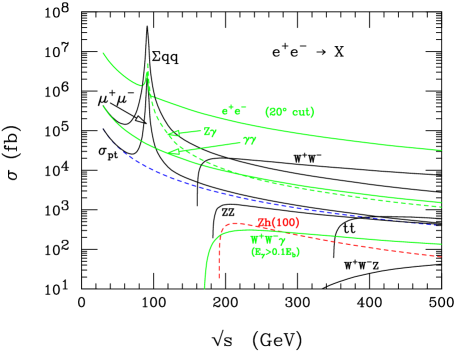
Figure 2: Representative SM production cross sections in $e^{+}e^{-}$ annihilation. For Bhabha scattering and final states involving photons, the differential cross sections $d\sigma/d\cos\theta$ have been integrated with a cut of $20^{o}<\theta<160^{o}$, in order to avoid the singular forward region. Note the $Z$ peak and the characteristic $1/s$ fall-off of cross sections at high energies.

The most direct and cleanest way to provide these high energies and luminosities is in $e^{+}e^{-}$ collisions. For most of the nineties, LEP at CERN and the SLAC linear collider (SLC) have operated on the $Z$ peak, at $\sqrt{s}\approx m_{Z}=91.187$ GeV, collecting some $10^{7}$ $Z$ decays at LEP and several hundred thousand at SLC. The high counting rate provided by the $Z$ resonance (see Fig. 2) has allowed very precise measurements of the couplings of the $Z$ to the SM quarks and leptons. At the same time searches for new particles were conducted, and the fact that nothing was found excludes any new particle which could be pair-produced in $Z$ decays, i.e. which have normal gauge couplings to the $Z$ and have masses $M\mathrel{\raisebox{-2.58334pt}{$\stackrel{{\scriptstyle\textstyle<}}{{\sim}}$}}m_{Z}/2$. This includes fourth generation quarks and leptons and the charginos, sleptons and squarks of supersymmetry.[1]

Since 1996 the energy of LEP has been increased in steps, via 161, 172, and 183 GeV, to 189 GeV in 1998. About 250 pb^-1 of data have been collected by each of the four LEP experiments over this period, mostly at the highest energy point. The experiments have mapped out the $W^{+}W^{-}$ production threshold (see Fig. 2), measured the $W$ mass and $W$ couplings directly, searched for the Higgs and set new mass limits on other new particles (see Section 3).

Why has progress been so incremental? The main culprit is synchrotron radiation in circular machines. The centripetal acceleration of the electrons on their circular orbit leads to an energy loss which grows as $\gamma^{4}/R$, where $R$ is the bending radius of the machine, approximately 4.2 km at LEP, and $\gamma=E_{e}/m_{e}$ is the time dilatation factor for the electrons, which at LEP exceeds $10^{5}$. The small electron mass requires very large bending radii, which can be achieved with very modest bending magnets in the synchrotron. Scaling up LEP to higher energies soon leads to impossible numbers. A 1 TeV electron synchrotron with the same synchrotron radiation loss as LEP (about 2.8 GeV per turn at $\sqrt{s}=200$ GeV)[8] would have to be over 600 times larger. The future of $e^{+}e^{-}$ machines belongs to linear colliders, which do not reuse the accelerated electrons and positrons, but rather collide the beams once, in a very high intensity beam spot. The SLC has been the first successful machine of this type. The next linear collider (NLC) would be a 400 GeV to 1 TeV $e^{+}e^{-}$ collider with a luminosity in the 10–100 fb^-1 per year range. With continued cooperation of physicists worldwide, such a machine might become a reality within a decade.

The easiest way to get to larger center of mass energies is to use heavier beam particles, namely protons or anti-protons. Their 2000 times larger mass makes synchrotron radiation losses negligible, even for much higher beam energies. Thus, the energy of proton storage rings is limited by the maximum magnetic fields which can be achieved to keep the particles on their circular orbits, i.e. the beam momentum $p$ is limited by the relation

$$p=eBR\;.$$ (3)

The Tevatron at Fermilab is the highest energy $\bar{p}p$ collider at present, and so far has accumulated about 120 pb^-1 of data, at a $\bar{p}p$ center of mass energy of 1.8 TeV, in each of two experiments, CDF and D0. It was this data taking period in the mid-nineties, called run I, which led to the discovery of the top-quark (see Section 4). Note that the pair production of top-quarks, with a mass of $m_{t}=175$ GeV, will be possible at $e^{+}e^{-}$ colliders only in the NLC era. A higher luminosity run at 2 TeV, run II, is scheduled to collect 1–2 fb^-1 of data, starting in the spring of 2000. And before an NLC will be constructed, the LHC at CERN will start with $pp$ collisions at a c.m. energy of 14 TeV and with a luminosity of $10^{33}$–$10^{34}\;{\rm cm}^{-2}{\rm sec}^{-1}$, corresponding to 10–100 fb^-1 per year.

Given these much higher energies available at hadron colliders, why do we still invest in $e^{+}e^{-}$ machines? The problem with hadron colliders is that protons are composite objects, made out of quarks and gluons, and these partons only carry a fraction of the proton energy. In order to produce new heavy particles the c.m. energy in a parton-parton collision must be larger than the sum of the masses of the produced particles, and this becomes increasingly unlikely as the required energy exceeds some 10–20% of the collider energy. Most $pp$ or $\bar{p}p$ collisions are collisions between fairly low energy partons. Since the proton is a composite object, of finite size, the total $pp$ or $\bar{p}p$ cross section does not decrease with energy, in fact it grows logarithmically and reaches about 100 mb at LHC energies. The high energy parton-parton collisions, however, suffer from the $1/s$ suppression discussed before. Production cross sections for new particles are of order 1 pb (with large variations), i.e. $10^{-11}$ times smaller. At hadron colliders, one thus needs to identify one interesting event in a background of $10^{11}$ bad ones, which poses a daunting task to the experimentalists and their detectors. The much cleaner situation at $e^{+}e^{-}$ colliders can be appreciated from Fig. 2: backgrounds to new physics searches arise form processes like $e^{+}e^{-}\rightarrow q\bar{q}$, $e^{+}e^{-}\rightarrow W^{+}W^{-}$, or $e^{+}e^{-}\rightarrow Z\gamma$, with cross sections in the 1–100 pb region and thus not much larger than the expected signal cross sections.

Figure 3: Schematic drawing representing decay of a $W^{+}\rightarrow\bar{q}q$ with subsequent parton showering and hadronization, leading to a dijet signature for the $W$ in the detector.

Whether new particles are produced in $e^{+}e^{-}$ or $pp$ collisions, they are never expected to be seen directly in the detector. Expected lifetimes, $\tau$, and ensuing decay lengths, $\gamma c\tau$, are of nuclear scale and, therefore, only the decay products can be observed. A typical example is shown in Fig. 3. A $W$ boson has a decay width of $\Gamma_{W}\approx 2.1$ GeV and is depicted to decay into a $u\bar{d}$ quark pair (other decay modes are $e^{+}\nu_{e},\;\mu^{+}\nu_{\mu},\;\tau^{+}\nu_{\tau}$ and $c\bar{s}$). The produced quarks, of course, are not observable either, due to confinement, rather they emit gluons and quark-antiquark pairs, which eventually hadronize and form jets of hadrons containing pions, kaons, and so on. The detectors have to observe these hadrons, measure the directions and energies of the jets, and deduce from here the four-momenta of the original $W^{+}$ or $u$ and $\bar{d}$ quarks.

The situation is very similar for other new heavy quanta. A Higgs boson, of mass $m_{H}=120$ GeV say, is expected to decay into $b\bar{b}$, $\tau^{+}\tau^{-}$ or $\gamma\gamma$, among others, with expected branching ratios

$$B(H\rightarrow b\bar{b}) = 74\%$$ (4)

$$B(H\rightarrow\tau^{+}\tau^{-}) = 6\%$$ (5)

$$B(H\rightarrow\gamma\gamma) = 0.2\%\;.$$ (6)

At LEP2, $ZH$ production is searched for in the $b\bar{b}$ decay mode of the Higgs, i.e. $b$-quark jets need to be observed and distinguished from lighter quark jets.

Supersymmetric particles are expected to produce an entire decay chain before they can be observed in the detector, an example being the decay of a gluino to a squark and a quark, where the squark in turn decays to the lightest neutralino, $\tilde{\chi}^{0}$ or chargino, $\tilde{\chi}^{\pm}$,

$$\tilde{g} \rightarrow \tilde{q}\bar{q}\rightarrow\bar{q}q\tilde{\chi}^{0}\rightarrow jj/\!\!\!E_{T}\;,$$ (7)

$$\tilde{g} \rightarrow \tilde{q}\bar{q}\rightarrow\bar{q}q^{\prime}\tilde{\chi}^{\pm}\rightarrow\bar{q}q^{\prime}W^{\pm}\tilde{\chi}^{0}\rightarrow\bar{q}q^{\prime}\ell^{\pm}\nu\tilde{\chi}^{0}\rightarrow jj\ell^{\pm}/\!\!\!E_{T}\;.$$ (8)

In the last step of the decay chain, hadronization of the quarks leads to jets, and the neutrino and the neutralino escape the detector, leading to an imbalance in the measured momenta of observable particles transverse to the beam, i.e. to a missing $E_{T}$ signature.

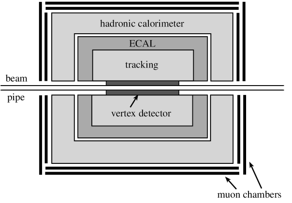
Figure 4: Schematic cross section through a typical collider detector. Shown, from the beam pipe out, are the locations of vertex detector, tracker, electromagnetic calorimeter, hadronic calorimeter, and muon chambers.

Collider detectors, which are to discover these new particles, must be designed to observe the decay products, positively identify them and measure their direction and their energy in the lab, i.e. determine the momenta of electrons, muons, photons and jets. In addition, the identification of heavy quarks, in particular the $b$ quarks arising in Higgs boson and top quark decays, is very important. Many technical solutions have been developed for this purpose, variations in the type of detector doing the reconstruction of charged particle tracks, or the energy measurement of electrons and photons (via electromagnetic showers) or jets (in a hadronic calorimeter). The basic layout of modern collider detectors is remarkably uniform, however, for fundamental physics reasons. For the basic level addressed in these lectures, it is sufficient to have a brief look at these common, global features.

The schematic drawing of Fig. 4 shows a cross section through a typical collider detector. The detector has a cylindrical structure, which is wrapped around the beam pipe in which the electrons or protons collide, at the center of the detector. The standard components of the detector are as follows.

• Central Tracking: The innermost part of the detector, closest to the interaction region, records the tracks of the produced charged particles, $e^{\pm}$, $\mu^{\pm}$, $\pi^{\pm}$, $K^{\pm}$ and so on. Via the bending of the tracks in a strong magnetic field, pointing along the beam direction, it measures the charged particle momenta.

• Electromagnetic Calorimeter: Neutral particles leave no tracks. They need to be measured via total absorption of their energy in a calorimeter. Electrons and photons loose their energy relatively quickly, via an electromagnetic shower. Since a shower develops randomly, statistical fluctuations limit the accuracy of the energy measurement. Excellent results, such as for the CMS detector at the LHC,[10] are

  $${\Delta E\over E}={0.02\over\sqrt{E}}\quad{\rm to}\quad{0.05\over\sqrt{E}}\;,$$ (9)

  where the energy $E$ is measured in GeV. Note that neutral pions decay into two photons before they leave the beam pipe, and these photons will stay very close to each other for large $\pi^{0}$ momentum. Hence, $\pi^{0}$s will be recorded in the electromagnetic calorimeter and they can fake photons.

• Hadronic Calorimeter: Other hadrons are absorbed in the hadron calorimeter where their energy deposition is measured, with a statistical error which may reach [9]

  $${\Delta E\over E}={0.4\over\sqrt{E}}\;.$$ (10)

  Typical hadron calorimeters have a thickness of some 25 absorption lengths and normally only muons, which do not interact strongly with the heavy nuclei of the hadron calorimeter, will penetrate it. Outside the calorimeter one therefore places the

• Muon Chambers: They record the location where a penetrating particle leaves the inner detector, and in several layers follows the direction of the track. Together with the central tracking information, this allows to measure the curvature of the muon track in the known magnetic fields inside the detector and determines the muon momentum.

• Vertex Detector: Bottom and charm quarks can be identified by the finite lifetime, of order 1 ps, of the hadrons which they form. This lifetime leads to a decay length of up to a few mm, i.e. the $b$ or $c$ decay products do not point back to the primary interaction vertex, which is much smaller, but to a secondary vertex. The decay length can be resolved with very high precision tracking. For this purpose modern collider detectors possess a solid state micro-vertex detector, very close to the beam-pipe, which provides information on the location of tracks with a resolution of order 10 $\mu$m. This technique now allows to identify centrally produced $b$-quarks, i.e. those that are produced at angles of more than a few degrees with respect to the beams, with efficiencies above 50% and with high purity, rejecting non-$b$ jets with more than 95% probability.

The various elements of the detector work together to identify the components of an event. An electron would deposit its energy in the electromagnetic calorimeter and produce a central track, which distinguishes it from a neutral photon. A charged pion or kaon produces a track also, but only a fraction of its energy ends up in the electromagnetic calorimeter: most of it leaks into the hadronic calorimeter. A muon, finally, deposits little energy in either calorimeter, rather it leads to a central track and to hits in the muon chambers.

If this muon originates from a $b$-decay, it will be traveling in the same direction as other hadrons belonging to the $b$-quark jet. This muon is not isolated, as opposed to a muon from a decay $W\rightarrow\mu\nu$ which only has a small probability to travel into the same direction as the twenty or thirty hadrons of a typical jet. One thus obtains a very detailed picture of the entire event, and from this picture one needs to reconstruct what happened at the parton level.

3 $e^{+}e^{-}$ Colliders

A full event reconstruction is most easily done at an $e^{+}e^{-}$ collider where the beam particles are elementary objects, i.e. the entire energy of the collision can go into the production of heavy particles. In contrast, at hadron colliders, the additional partons in the parent protons lead to a spray of hadrons in the detector which obscure the parton-parton collision we are interested in.

In $e^{+}e^{-}$ collisions at energies $\sqrt{s}\mathrel{\raisebox{-2.58334pt}{$\stackrel{{\scriptstyle\textstyle<}}{{\sim}}$}}160$ GeV, the dominant hard process is fermion pair production, $e^{+}e^{-}\rightarrow\bar{f}f$. For $f=e,\;\mu$ this leads to extremely clean events with two particles in the final state only, and even the bulk of $\bar{q}q$ production events are easily recognized as dijet events. With the advent of LEP2 the situation has become more complicated. As can be seen in Fig. 2, $W^{+}W^{-}$ and $ZZ$ events are as copious as fermion pair production, but they lead to a more complex 4-fermion final state, via the decay of the two $W$s or $Z$s into a pair of quarks or leptons each. Let us start our survey of $e^{+}e^{-}$ physics with this new class of events, which will be important in all new high energy $e^{+}e^{-}$ colliders. They show interesting features and provide information on fundamental parameters of the SM in their own right, but also they form an important background to new particle searches, such as charginos for example, and we need to analyze them in some detail.

Figure 5: Feynman graphs for the process $e^{+}e^{-}\rightarrow W^{+}W^{-}$. The labels on the neutrino exchange graph give the particle momenta.

3.1 $W^{+}W^{-}$ production

At tree level, three Feynman graphs contribute to the production of $W$ pairs.[11, 12] They are $s$-channel $\gamma$- and $Z$-exchange, and $t$-channel neutrino exchange, and are shown in Fig. 5. The dominant features of the production cross section can be read off the propagator structure of the individual graphs. While the two $s$-channel amplitudes show a modest dependence on scattering angle only, the neutrino exchange graph produces a strong peaking at small scattering angles: the propagator factor for this graph is $1/t$ with $t=(p-k)^{2}=-2p\cdot k+m_{W}^{2}$. In the c.m. system we choose the initial electron momentum, $p$, along the $z$-axis and define the scattering angle as the angle between the $W^{-}$ and the $e^{-}$ direction, i.e.

$$p={\sqrt{s}\over 2}(1,0,0,1)\;,\qquad k={\sqrt{s}\over 2}(1,\beta\sin\theta,0,\beta\cos\theta)\;,$$ (11)

where $\beta=\sqrt{1-4m_{W}^{2}/s}$ is the velocity of the produced $W$. The denominator of the propagator then becomes

$$|t|={s\over 4}\left(2-2\beta\cos\theta-{4m_{W}^{2}\over s}\right)={s\over 4}\left(1+\beta^{2}-2\beta\cos\theta\right)\geq{s\over 4}\left(1-\beta\right)^{2}\;.$$ (12)

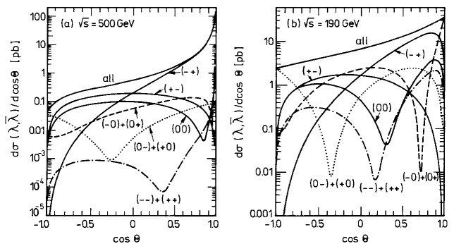
Figure 6: Angular distribution $d\sigma/d\cos\theta$ for $e^{+}e^{-}\rightarrow W^{+}W^{-}$ production at (a) $\sqrt{s}=500$ GeV and (b) $\sqrt{s}=190$ GeV, within the SM. Also shown are the cross sections for the various $W^{-}W^{+}$ helicity combinations $(\lambda,\bar{\lambda})$. Where a sum is shown, both helicity combinations give the same result. From Ref. [11].

Close to threshold, i.e. for $\beta\approx 0$, there is little angular dependence. At high energies, however, as $\beta\rightarrow 1$, $|t|$ becomes very small near $\theta=0$ and the $1/t$ pole induces a strongly peaked $W$ pair cross section near forward scattering angles. This effect is shown in Fig. 6, where the angular distribution $d\sigma/d\cos\theta$ for $W^{+}W^{-}$ production in the SM is shown, including the contributions from different $W^{-}$ and $W^{+}$ helicities, $\lambda$ and $\bar{\lambda}$. Angular momentum conservation and the fact that left-handed electrons only contribute to the $\nu$-exchange graph, lead to a strong polarization of the produced $W$’s in the forward region: the produced $W^{-}$ helicity is mostly $-1$ in this region, i.e. it picks up the electron helicity.

The $W$s are only observed via their decay products, $W\rightarrow\bar{f}f^{\prime}$, where three $\ell\nu$ combinations $(\ell=e,\mu,\tau)$ and six quark combinations can be produced ($u\bar{d}$ and $c\bar{s}$ and counting $N=3$ different colors). Since all quarks and leptons couple equally to $W$s (when neglecting Cabibbo mixing), and because any CKM effects exactly compensate in the decay widths, the branching ratios to leptons and hadrons are simply given by

$$B(W\rightarrow e\nu_{e})=B(W\rightarrow\mu\nu_{\mu}) = B(W\rightarrow\tau\nu_{\tau})={1\over 9}\;,$$ (13)

$$B(W\rightarrow{\rm hadrons}) = {1\over 9}\cdot 2\cdot 3={2\over 3}\;.$$ (14)

QCD effects induce corrections of a few percent to these relations. In lowest order, a decay $W\rightarrow\bar{q}q^{\prime}$ leads to two jets in the final state, and this, combined with the branching ratios of Eq. (13,14), fixes the probabilities for the various classes of events to be observed for $W^{+}W^{-}$ production,

$$B(W^{+}W^{-}\rightarrow{4\rm jets}) = 46\%\;,$$ (15)

$$B(W^{+}W^{-}\rightarrow jj+e\nu_{e},\mu\nu_{\mu}) = 29\%\;,$$ (16)

$$B(W^{+}W^{-}\rightarrow\ell^{+}\nu\ell^{-}\bar{\nu}) = 10.5\%\;,$$ (17)

$$B(W^{+}W^{-}\rightarrow jj+\tau\nu_{\tau}) = 14.5\%\;.$$ (18)

Thus, it is most likely to observe the two $W$s in 4-jet events, followed by the ‘semileptonic’ channel, where one $W$ decays into either electrons or muons. The remaining channels have at least two neutrinos in the final state (the $\tau$ decays inside the beam-pipe!) and hence a substantial fraction of the final state particles cannot be observed, which limits the reconstruction of the event. Fortunately, these more difficult situations comprise only one quarter of the $W$ pair sample.

Figure 7: Orientation of spins for the decay of a right-handed $W^{-}$ into a pair of fermions, $f_{1}\bar{f}_{2}$. Because of the $V-A$ structure of charged currents, the fermion helicities are fixed as shown.

As we saw when discussing production angular distributions, the $W$s are strongly polarized. Fortunately, the $V-A$ structure of the $W$-fermion couplings provides a very efficient polarization analyzer for the $W$s, via their decay distributions. Consider the decay of a right-handed $W^{-}$, i.e. of helicity $\lambda=+1$, as depicted in Fig. 7 in the $W$ rest frame. Because of the $V-A$ coupling, the decay $W\rightarrow f_{1}\bar{f}_{2}$ always leads to a left-handed fermion and a right-handed anti-fermion, in the massless fermion limit. The fermion spins therefore always line up as shown in the figure. Taking the decay polar angle $\theta_{1}^{*}\rightarrow 0$, the combined fermion spins point opposite to the spin of the parent $W^{-}$. Angular momentum conservation does not allow this, which means that the decay amplitude vanishes at $\cos\theta_{1}^{*}=1$. The same argument shows that for a left-handed $W^{-}$, of helicity $\lambda=-1$, the decay amplitude must vanish for $\cos\theta_{1}^{*}=-1$. A quick calculation shows that the decay amplitudes for $W^{-}\rightarrow f_{1}\bar{f}_{2}$ are proportional to

$$D(W^{-}\rightarrow f_{1}\bar{f}_{2})(\lambda=+1) = {1\over\sqrt{2}}\left(1-\cos\theta_{1}^{*}\right)e^{i\phi_{1}^{*}}\;,$$ (19)

$$D(W^{-}\rightarrow f_{1}\bar{f}_{2})(\lambda=0) = -\sin\theta_{1}^{*}\;,$$ (20)

$$D(W^{-}\rightarrow f_{1}\bar{f}_{2})(\lambda=-1) = {1\over\sqrt{2}}\left(1+\cos\theta_{1}^{*}\right)e^{-i\phi_{1}^{*}}\;,$$ (21)

where $\phi_{1}^{*}$ is the decay azimuthal angle, as indicated in the figure. Analogous results are obtained, of course, for the $W^{+}$ decay angles $\theta_{2}^{*}$ and $\phi_{2}^{*}$.

By measuring the decay angular distributions, i.e. by distinguishing the $(1-\cos\theta^{*})^{2}$, $\sin^{2}\theta^{*}$, and $(1+\cos\theta^{*})^{2}$ distributions for right-handed, longitudinal and left-handed polarized $W$s, we can measure the average $W$ polarization. The full polarization information is contained in the 5-fold production and decay angular distributions,[11, 12, 13]

$${d^{5}\sigma\over d\cos\theta\;d\cos\theta_{1}^{*}\;d\phi_{1}^{*}\;d\cos\theta_{2}^{*}\;d\phi_{2}^{*}}\;,$$ (22)

Here the decay angles are defined in the $W^{-}$ and $W^{+}$ rest frames, respectively, and are measured against the direction of the parent $W$ in the lab.

A major reason to study this 5-fold angular distribution is the experimental determination of the $WWZ$ and $WW\gamma$ couplings which enter in the first two Feynman graphs of Fig. 5. This is analogous to the measurement of vector and axial vector couplings of the various fermions to the $Z$ and the $W$. The experiments at LEP2 so far confirm the SM predictions for these triple-gauge-boson couplings at about the 10% level.[13, 14]

Why would one consider $W$ decay angular distributions if one does not want to measure polarizations or triple-gauge-boson couplings? As we saw when discussing $W$ production, the produced $W^{-}$ is very strongly left-handed polarized in the forward direction. This polarization has important consequences for the energy distribution of the decay products, and therefore for the way the event appears in the detector. To be definite, let us consider the decay $W^{-}\rightarrow\ell^{-}\bar{\nu}$. In the $W$ rest frame, the four-momentum of the charged lepton is given by

$$p^{*}={m_{W}\over 2}\left(1,\sin\theta_{1}^{*}\cos\phi_{1}^{*},\sin\theta_{1}^{*}\sin\phi_{1}^{*},\cos\theta_{1}^{*}\right)\;.$$ (23)

The charged lepton energy in the lab frame is obtained from here via a boost of its four-momentum, with a $\gamma$-factor $\gamma=E_{W}/m_{W}=\sqrt{s}/2m_{W}$,

$$p^{0}=\gamma\bigl{(}p^{0*}+\beta p_{z}^{*}\bigr{)}=\gamma{m_{W}\over 2}\bigl{(}1+\beta\cos\theta_{1}^{*}\bigr{)}={\sqrt{s}\over 4}\bigl{(}1+\beta\cos\theta_{1}^{*}\bigr{)}\;.$$ (24)

Thus, the polar angle of the lepton in the $W$ rest frame can be measured in terms of the lepton energy in the lab frame, and the two observables directly correspond to each other. This also implies that the energy distributions of the leptons in the lab are determined by their angular distributions in the $W$ rest frame, and these are fixed by the polarization of the parent $W$.

As a concrete example, consider the average energy of the charged lepton, for the decay of a left-handed $W^{-}$. We need to average the result of Eq. (24) over the normalized decay angular distribution, $3/8(1+\cos\theta^{*})^{2}$, for a left-handed $W^{-}$:

$$\left<p^{0}(\ell^{-})\right>={E_{W}\over 2}\int^{1}_{-1}d\cos\theta^{*}{3\over 8}(1+\cos\theta^{*})^{2}(1+\beta\cos\theta^{*})={E_{W}\over 2}(1+{\beta\over 2})\;.$$ (25)

Energy conservation fixes the average neutrino momentum to

$$\left<p^{0}(\nu)\right>={E_{W}\over 2}(1-{\beta\over 2})\;.$$ (26)

In the relativistic limit, $\beta\rightarrow 1$, the neutrino receives only 1/3 of the energy of the charged lepton, on average, which has important consequences for detection and energy measurement of the leptons as well as for the consideration of $W$ pair production as backgrounds to new physics searches.

Polarization effects can have dramatic effects and one therefore needs predictions for $W$ pair production and decay which consider the full chain $e^{+}e^{-}\rightarrow W^{+}W^{-}\rightarrow{4\;\rm fermions}$. In this full $2\rightarrow 4$ process the $W$s merely appear as resonant propagators, which are treated as Breit-Wigner resonances. Away from the peak of the resonance, seven additional Feynman graphs contribute, beyond the three shown in Fig. 5, even for the simplest case, $e^{+}e^{-}\rightarrow\mu^{-}\bar{\nu}_{\mu}\;u\bar{d}$. These calculations have been performed [12] and are being used in the actual data analysis.

Another application, which nicely demonstrates the advantages of $e^{+}e^{-}$ collisions, is the $W$-mass measurement in $W^{+}W^{-}$ production at LEP2.[15] Let us consider the decay $W^{+}W^{-}\rightarrow\ell\nu jj$ as an example. A full reconstruction of the Breit-Wigner resonances, and a measurement of its center, at $m_{W}$, is possible with the two jet momenta. However, the measurements of the jets’ energies have large errors, of order $\pm 15\%$, and such a direct approach would lead to fairly large errors on the extracted $W$-mass. One can do much better by making use of the known kinematics of the event.

The 3-momentum of the neutrino in the event can be reconstructed from momentum conservation, as

$${\bf p}_{\nu}=-{\bf p}_{\ell}-{\bf p}_{j_{1}}-{\bf p}_{j_{2}}\;,$$ (27)

where we have used the fact that the lab frame is the c.m. frame, i.e. the sum of all the final state momenta in the lab must add up to zero. The energy of the massless neutrino is then given by $E_{\nu}=|{\bf p}_{\nu}|$. Energy conservation and the equal masses of the two $W$s now imply the constraints

$$E_{W_{1}}=E_{j_{1}}+E_{j_{2}}=E_{b}\;,\qquad E_{W_{2}}=E_{\ell}+E_{\nu}=E_{b}\;,$$ (28)

where $E_{b}=\sqrt{s}/2$ is the beam energy. Even when considering the finite widths of the $W$ resonances and the possibility of initial state radiation, i.e. emission of photons along the beam direction, which effectively lowers the c.m. energy $\sqrt{s}$, the constraint of Eq. (28) is satisfied to much higher accuracy than the precision of the jet energy measurement. One can thus drastically improve the $W$-mass resolution by using the two constraints to solve for the two unknowns $E_{j_{1}}$ and $E_{j_{2}}$ and use these values to calculate the $W^{+}$ and $W^{-}$ mass. The expected improvement is illustrated in Fig. 8.

Figure 8: Expected $W$-mass reconstruction in $W^{+}W^{-}\rightarrow\ell\nu jj$ events at LEP2. The two plots show the invariant mass distribution of the $W$ decay products before and after using the kinematic constraints described in the text. From Ref. [15].

First measurements of the $W$-mass, using both $\ell\nu jj$ and 4-jet events, have already been performed with the 172 and 183 GeV data and resulted in [16]

$$m_{W}=80.36\pm 0.09\;{\rm GeV}\;,$$ (29)

where the results from all four LEP experiments have been combined. Further improvements are expected in the near future from the four times larger event sample already collected in 1998. The LEP value agrees well with the one extracted from order $10^{5}$ leptonic $W$-decays observed at the Tevatron, $m_{W}=80.41\pm 0.09$ GeV.[17]

3.2 Chargino pair production

So far we have considered $W^{+}W^{-}$ production as a signal. However, $W$-pairs can be a serious background in the search for other new particles. Let us consider one example in some detail, the production of charginos at LEP2.

Figure 9: Feynman graphs for (a) chargino production in $e^{+}e^{-}$ annihilation and (b) chargino decay into the lightest neutralino, $\tilde{\chi}^{0}_{1}$ and a pair of quarks or leptons.

Charginos arise in supersymmetric models [5] as the fermionic partners of the $W^{\pm}$ and the charged Higgs, $H^{\pm}$. Since they carry electric and weak charges, they couple to both the photon and the $Z$ and can be pair-produced in $e^{+}e^{-}$ annihilation. The relevant Feynman graphs are shown in Fig. 9(a). Note that the graphs for chargino production are completely analogous to the ones in Fig. 5 for $W$-pair production, a reflection of the supersymmetry of the couplings.

Two charginos are predicted by supersymmetry, and the lighter one, $\tilde{\chi}^{\pm}_{1}$, might be light enough to be pair-produced at LEP2.[18] Production cross sections can be sizable, ranging from 2 to 5 pb at LEP2 for typical parameters of SUSY models. However, the $s$-channel $\gamma$ and $Z$ exchange graphs, and $t$-channel sneutrino exchange in Fig. 9(a), interfere destructively. For small sneutrino masses, of order 100 GeV or less, this can lead to a drastic reduction in the chargino pair production cross section, in particular near threshold. As a result, one must be prepared for production cross sections well below 1 pb at LEP2 also. In any case, the expected chargino pair cross section can be smaller than the cross section for the dominant background, $\sigma(e^{+}e^{-}\rightarrow W^{+}W^{-})\approx 17$ pb, by one order of magnitude or more.

A chargino, once it is produced, is expected to decay into the lightest neutralino, $\tilde{\chi}_{1}^{0}$, and known quarks and leptons, as shown in Fig. 9(b). The lightest neutralino is stable in most SUSY models, due to conserved $R$-parity, and does not interact inside the detector, thus leading to a missing momentum signature. Over large regions of parameter space, where the squarks and sleptons entering the chargino decay graphs are quite heavy, the chargino effectively decays into the neutralino and a virtual $W$. This results in a signature which is quite similar to $W$-pair production, since only the $W^{*}$ decay products are seen inside the detector. Thus, LEP looks for the charginos via the production and decay chain

$$e^{+}e^{-}\rightarrow\tilde{\chi}_{1}^{+}\tilde{\chi}_{1}^{-}\rightarrow\tilde{\chi}_{1}^{0}\tilde{\chi}_{1}^{0}W^{+*}W^{-*}\;,$$ (30)

which, just like $W^{+}W^{-}$ production, leads to a $jjjj$ signature 46% of the time and to an $\ell\nu jj$ final state (including $\tau$’s) in 43.5% of all cases. The only difference is the additional presence of two massive neutralinos, which needs to be exploited.

Since the neutralinos escape detection, the energy deposited in the detector typically is less than for $W^{+}W^{-}$ events. In addition, the missing neutralinos spoil the momentum balance of the visible particles, which leads to a more spherically symmetric event than encountered in $W$ pair production. The most effective cut arises from the fact, however, that the four-momentum of the missing neutrinos and neutralinos can be reconstructed due to the beam constraint. Four-momentum conservation for the $\ell\nu jj\tilde{\chi}^{0}\tilde{\chi}^{0}$ final state state reads

$$p_{e^{-}}+p_{e^{+}}=p_{\ell}+p_{j_{1}}+p_{j_{2}}+/\!\!\!p\;$$ (31)

from which the missing mass, $M_{\rm miss}^{2}=/\!\!\!p^{2}$ can be reconstructed. For a $W^{+}W^{-}$ event the missing momentum corresponds to a single neutrino and, thus, $M_{\rm miss}=0$. For the signal, however, one has

$$/\!\!\!p^{2}>4m_{\tilde{\chi}^{0}}^{2}\;.$$ (32)

Not only does the consideration of the missing mass allow for effective background reduction, to a level below 0.05–0.1 pb,[18] but it would also provide a measurement of the lightest neutralino mass, once charginos are discovered.

So far, no chargino signal has been observed at LEP. This pushes the chargino mass bound above 90 GeV, provided the chargino-neutralino mass difference is sufficiently large to allow enough energy for the visible chargino decay products.[19] The LEP experiments have searched for other super-partners also, like squarks and sleptons, and have not yet discovered any signals. The sfermions, since they are scalars, have a softer threshold turn-on, proportional to $\beta^{3}$, and hence have a very low pair production cross section if their mass is close to the beam energy. As a result, squark and slepton mass bounds currently are somewhat weaker than for charginos, but even here, sfermions with masses below 70–85 GeV (depending on flavor) are excluded.[19]

3.3 Future $e^{+}e^{-}$ and $\mu^{+}\mu^{-}$ colliders

An exciting search presently being conducted at LEP is the hunt for the Higgs boson, in $e^{+}e^{-}\rightarrow ZH$.[22] The mass of the Higgs boson does influence radiative corrections to 4-fermion amplitudes, via $ZH$ and $WH$ loops contributing to the $Z$ and $W$ propagator corrections. Precise measurements of asymmetries in $e^{+}e^{-}\rightarrow\bar{f}f$, of partial $Z$ widths to leptons and quarks, of atomic parity violation etc. allow to extract the expected Higgs mass within the SM. These measurements point to a relatively small Higgs mass, of about 100 GeV, albeit with a large error of about a factor of two.[1, 20, 21] LEP is exactly searching in this region.

In $e^{+}e^{-}\rightarrow ZH$, the large mass of the accompanying $Z$ limits the reach of the LEP experiments, to about [22]

$$m_{H}\mathrel{\raisebox{-2.58334pt}{$\stackrel{{\scriptstyle\textstyle<}}{{\sim}}$}}\sqrt{s}-m_{Z}-5\;{\rm GeV}\;.$$ (33)

With an eventual c.m. energy of $\sqrt{s}\approx 200$ GeV, this allows discovery of the Higgs at LEP, provided its mass is below about 105 GeV. However, measurements at energies up to 189 GeV have not discovered anything yet, setting a lower Higgs mass bound, within the SM, of 95 GeV.[21] We need luck to still find a Higgs signal at LEP, before the LEP tunnel needs to be cleared for installing the LHC.

Given the indications for a relatively light Higgs from electroweak precision data, an expectation which is shared by supersymmetric models,[5] an $e^{+}e^{-}$ collider with higher c.m. energy than LEP2 is called for. As explained in Section 2 this cannot be a circular machine, due to excessive synchrotron radiation, but rather should be a linear $e^{+}e^{-}$ collider.[23] A 500 GeV NLC, with a yearly integrated luminosity of 10–100 fb^-1, would be a veritable Higgs factory. At such a machine, the Higgs production cross section is of order 0.1 pb in both the $e^{+}e^{-}\rightarrow ZH$ production channel (for $m_{H}\mathrel{\raisebox{-2.58334pt}{$\stackrel{{\scriptstyle\textstyle<}}{{\sim}}$}}300$ GeV) and also in the weak boson fusion channel, where the Higgs boson is radiated off a $t$-channel $W$ ($\sigma(e^{+}e^{-}\rightarrow H\nu\bar{\nu})\mathrel{\raisebox{-2.58334pt}{$\stackrel{{\scriptstyle\textstyle>}}{{\sim}}$}}0.03$ pb for $m_{H}\mathrel{\raisebox{-2.58334pt}{$\stackrel{{\scriptstyle\textstyle<}}{{\sim}}$}}200$ GeV). In this mass range, the 1000 to 10000 produced Higgs bosons per year would allow for detailed investigations of Higgs boson properties, in the clean environment of an $e^{+}e^{-}$ collider. Somewhat higher Higgs boson masses, up to $m_{H}\approx\sqrt{s}-100$ GeV (see Eq. (33)) are accessible as well, albeit with lower production rates.

The NLC would greatly extend the search region for other new heavy particles as well, like the charginos and neutralinos of the MSSM, or its squarks and sleptons. Even if theses particles are first discovered at a hadron collider like the LHC, the cleaner environment of $e^{+}e^{-}$ collisions, the more constrained kinematics, and the observability of most of the decay channels give linear $e^{+}e^{-}$ colliders great advantages for detailed studies of the properties of any new particles.

This is true also for the latest new particle that has been discovered already, the top quark.[24, 25] A scan of the top production threshold in $e^{+}e^{-}$ collisions, at $\sqrt{s}=2m_{t}\approx 350$ GeV, would give an unprecedented precision in the measurement of the top quark mass. The simultaneous direct measurement of the top quark width would determine the $V_{tb}$ CKM matrix element and thus provide a significant test of the electroweak sector.

All these $e^{+}e^{-}$ collider measurements could also be performed at a $\mu^{+}\mu^{-}$ collider.[6] Such a machine would have the added advantage of an excellent beam energy resolution, of order $10^{-4}$ or better, while beam-strahlung in the tight focus of an $e^{+}e^{-}$ linear collider leads to a significant smearing of the c.m. energy. The very precisely determined beam energy can then be used for a scan of the $\bar{t}t$ production threshold, which resolves detailed features like the location of the (extremely short-lived) first $\bar{t}t$ bound state, QCD binding effects and the value of the strong coupling constant, or even Higgs exchange effects on the shape of the $\bar{t}t$ production threshold.

Another advantage of a $\mu^{+}\mu^{-}$ collider is the larger coupling of the Higgs boson to the muon as compared to the electron, due to the muon’s 200 times larger mass. This allows the direct $s$-channel production of the Higgs resonance in muon collisions, $\mu^{+}\mu^{-}\rightarrow H$. Because of the excellent energy resolution of a muon collider, an energy scan of the Higgs resonance would provide us with a very precise measurement of the Higgs boson mass, with an error of order MeV, and if dedicated efforts are made to keep the energy spread as small as possible, even the full width of the Higgs resonance can be determined directly.[6]

These examples clearly show that a linear $e^{+}e^{-}$ collider or a muon collider would be a terrific experimental tool and would greatly advance our understanding of particle interactions. Unfortunately, no such machine has been approved for construction yet. And it may be argued that we first need to establish the existence of new heavy particles before investing several billion dollars or euros into a machine to search for them and then study their detailed properties. For many of the particles predicted by supersymmetry, or for the Higgs boson, the machines needed for discovery already exist or are under construction, namely the Tevatron at Fermilab and the LHC at CERN.

4 Hadron Colliders

The highest center of mass energies and, hence, the best reach for new heavy particles is provided by hadron colliders, the Tevatron with its 2 TeV $\bar{p}p$ collisions at present, and the LHC with 14 TeV $pp$ collisions after 2005. At the Tevatron the top quark has been discovered in 1994, and Higgs and supersymmetry searches will resume in run II. The LHC is expected to do detailed investigations of the Higgs sector, and should answer the question whether TeV scale supersymmetry is realized in nature. Before discussing how these studies can be performed in a hadron collider environment, we need to consider the general properties of production processes at these machines in some detail.

4.1 Hadrons and partons

A typical hard hadronic collision is sketched in Fig. 10: one of the subprocesses contributing to $Z+$jet production, namely $ug\rightarrow uZ$. The up-quark and the gluon carry a fraction of the parent proton momenta only, $x_{1}$ and $x_{2}$, respectively. Thus, the incoming parton momenta are given by

$$p_{u} = x_{1}p=x_{1}{\sqrt{s}\over 2}\bigl{(}1,0,0,1)\;,$$

$$p_{g} = x_{2}\bar{p}=x_{2}{\sqrt{s}\over 2}\bigl{(}1,0,0,-1)\;,$$ (34)

and the available center of mass energy for the $Z+$jet final state is given by the root of $\hat{s}=(p_{u}+p_{g})^{2}=2p_{u}\cdot p_{g}=x_{1}x_{2}s$, i.e. it is only a fraction $\sqrt{x_{1}x_{2}}$ of the collider energy.

Figure 10: One of the subprocesses contributing to $Zj$ production in $p\bar{p}$ collisions. The two initial partons carry momentum fractions $x_{1}$ and $x_{2}$ of the incoming proton and anti-proton, respectively.

In order to calculate observable production rates, for a process $p\bar{p}\rightarrow X$, we first need to identify all the parton level subprocesses $a_{1}+a_{2}\rightarrow\hat{x}=b_{1}+b_{2}+\cdots+b_{n}$ which give the desired signature. In the above example of $Z+$jet production this includes, at tree level, $u+\bar{u}\rightarrow Z+g$, $\bar{u}+u\rightarrow Z+g$ (i.e. the subprocess where the anti-$u$ comes from the proton), $g+u\rightarrow Z+u$, $u+g\rightarrow Z+u$, $g+\bar{u}\rightarrow Z+\bar{u}$, $\bar{u}+g\rightarrow Z+\bar{u}$, and all the corresponding subprocesses with the up quark replaced by down, strange, charm, and bottom quarks, which are all treated as massless partons inside the proton. The full cross section for the process $p\bar{p}\rightarrow X$ is then given by

$$\sigma = \int dx_{1}dx_{2}\sum_{\rm subprocesses}\;f_{a_{1}/p}(x_{1})\;f_{a_{2}/\bar{p}}(x_{2})\;$$ (35)

$${1\over 2\hat{s}}\int d\Phi_{n}(x_{1}p+x_{2}\bar{p};\;p_{1}\dots p_{n})\Theta({\rm cuts})$$

$$\overline{\sum}|{\cal M}|^{2}(a_{1}a_{2}\rightarrow b_{1}b_{2}\dots b_{n})\;.$$

Here $f_{a_{1}/p}(x_{1})$ is the probability to find parton $a_{1}$ inside the proton, carrying a fraction $x_{1}$ of the proton momentum, i.e. the $a_{1}$ parton distribution function. Similarly, $f_{a_{2}/\bar{p}}(x_{2})$ is the $a_{2}$ parton distribution function (pdf) inside the anti-proton. In the second line of (35) $1/2\hat{s}$ is the flux factor for the partonic cross section,

$$d\Phi_{n}(P;\;p_{1}\dots p_{n})=\prod_{i=1}^{n}\left({d^{3}{\bf p}_{i}\over(2\pi)^{3}2E_{i}}\right)(2\pi)^{4}\;\delta^{4}(P-\sum_{i}p_{i})$$ (36)

is the Lorentz invariant phase space element, and $\Theta({\rm cuts})$ is the acceptance function, which summarizes the kinematical cuts on all the final state particles, i.e. $\Theta=1$ if all the partons $a_{i}$ satisfy all the acceptance cuts and $\Theta=0$ otherwise. Finally, ${\cal M}$, in the third line of (35) is the Feynman amplitude for the subprocess in question, squared and summed/averaged over the polarizations and colors of the external partons.

Compared to the calculation of cross sections for $e^{+}e^{-}$ collision, the new features are integration over pdf’s and the fact that a much larger number of partonic subprocesses must be considered for a given experimental signature. The introduction of pdf’s introduces an additional uncertainty since they need to be extracted from other data, like deep inelastic scattering, $W$ production at the Tevatron, or direct photon production. The extraction of pdf’s is continuously being updated and refined, and in practice, hadron collider cross sections are calculated by using numerical interpolations which are provided by the groups improving the pdf sets.[26] These pdf determinations have been dramatically improved over time and typical pdf uncertainties now are below the 5% level, at least in the range $10^{-3}\mathrel{\raisebox{-2.58334pt}{$\stackrel{{\scriptstyle\textstyle<}}{{\sim}}$}}x\mathrel{\raisebox{-2.58334pt}{$\stackrel{{\scriptstyle\textstyle<}}{{\sim}}$}}0.2$, which is most important for our discussion of new particle production processes.

More important than the appearance of pdf’s are the kinematic effects which result from the fact that the hard collision is between partons. Since momenta of the incoming partons are not known a priori, we cannot make use of a beam energy constraint as in the case of $e^{+}e^{-}$ collisions. The missing information on the momentum parallel to the beam axis affects the analysis of events with unobserved particles in the final state, like neutrinos or the lightest neutralino. Momentum conservation can only be used for the components transverse to the beam axis, i.e. only the missing transverse momentum vector, ${/\!\!\!\bf p}_{T}$, can be reconstructed.

Another effect is that the lab frame and the c.m. frame of the hard collision no longer coincide. Rather the partonic c.m. system receives a longitudinal boost in the direction of the beam axis, which depends on $x_{1}/x_{2}$. This longitudinal boost is most easily taken into account by describing four-momenta in terms of rapidity $y$ instead of scattering angle $\theta$. For a momentum vector

$$p=(E,p_{x},p_{y},p_{z})=E(1,\beta\sin\theta\cos\phi,\beta\sin\theta\sin\phi,\beta\cos\theta)\;,$$ (37)

rapidity is defined as

$$y={1\over 2}\log{E+p_{z}\over E-p_{z}}\;,$$ (38)

which, in the massless limit ($\beta\rightarrow 1$), reduces to pseudo-rapidity,

$$\eta={1\over 2}\log{1+\cos\theta\over 1-\cos\theta}\;.$$ (39)

The advantage of using rapidity is that under an arbitrary boost along the $z$-axis, rapidity differences remain invariant, i.e. they directly measure relative scattering angles in the partonic c.m. frame. Using Eq. (34), the c.m. momentum is given by $P=\sqrt{s}/2(x_{1}+x_{2},0,0,x_{1}-x_{2})$ which results in a c.m. rapidity $y_{c.m.}=1/2\log(x_{1}/x_{2})$. As a result, rapidities $y^{*}$ in the partonic c.m. system and rapidities $y$ in the lab frame are connected by

$$y=y^{*}+y_{c.m.}=y^{*}+{1\over 2}\log{x_{1}\over x_{2}}\;,$$ (40)

a relation which can be used to determine all scattering angles in the theoretically simpler partonic rest frame whenever all final state momenta can be measured and, hence, the c.m. momentum $P$ is known.

4.2 $Z$ and $W$ Production

One of the early highlights of $\bar{p}p$ colliders was the discovery of the $W$ and $Z$ bosons at the CERN S$\bar{p}p$S, a 630 GeV $\bar{p}p$ collider.[27] $W$ and $Z$ production provide a nice example which demonstrates the use of some of the transverse observables discussed in the previous subsection. In addition, the story might repeat, since nature might have an additional neutral or charged heavy gauge boson in store, a $Z^{\prime}$ or an $W^{\prime}$ which might appear at the LHC. Let us thus consider $Z$ production in some detail.

The prototypical Drell-Yan process is $\bar{p}p\rightarrow Z\rightarrow\ell^{+}\ell^{-}$, where, to lowest order in the strong coupling constant, the $Z$ can be produced by annihilation of a quark-antiquark pair . The partonic subprocess $\bar{q}q\rightarrow\ell^{+}\ell^{-}$ leads to two leptons with balancing transverse momenta, which can be parameterized in terms of their lab frame $p_{T}$, pseudo-rapidity $\eta$, and azimuthal angle $\phi$,

$$\ell = p_{T}\bigl{(}\cosh\eta,\cos\phi,\sin\phi,\sinh\eta\bigr{)}\;,$$ (41)

$$\bar{\ell} = p_{T}\bigl{(}\cosh\bar{\eta},-\cos\phi,-\sin\phi,\sinh\bar{\eta}\bigr{)}\;.$$ (42)

Since transverse momentum is invariant under a boost along the $z$-axis, we may as well determine it in the partonic c.m. frame, where the $\ell^{-}$ momentum is given by

$$\ell^{*}={m_{Z}\over 2}\bigl{(}1,\sin\theta^{*}\cos\phi,\sin\theta^{*}\sin\phi,\cos\theta^{*}\bigr{)}\;.$$ (43)

One finds $p_{T}=m_{Z}/2\;\sin\theta^{*}$ by equating the transverse momenta in the two frames. This implies

$$|\cos\theta^{*}|=\sqrt{1-\sin^{2}\theta^{*}}=\sqrt{1-{4p_{T}^{2}\over m_{Z}^{2}}}\;.$$ (44)

Using this relation we obtain the transverse momentum spectrum in terms of the lepton angular distribution in the c.m. frame,

$${d\sigma\over dp_{T}^{2}}={d\sigma\over d\cos\theta^{*}}\left|{d\cos\theta*\over dp_{T}^{2}}\right|={d\sigma\over d\cos\theta^{*}}{1\over m_{Z}\sqrt{m_{Z}^{2}/4-p_{T}^{2}}}\;.$$ (45)

The $p_{T}$ distribution diverges at the maximum transverse momentum value, $p_{T}=m_{Z}/2$. This Jacobian-peak, so called because it arises from the Jacobian factor in Eq. (45), is smeared out in practice by finite detector resolution, the finite $Z$-width and QCD effects. Nevertheless, it is an excellent tool to determine the $W$ mass in the analogous $W\rightarrow\ell\nu$ decay, which has the Jacobian peak at half the $W$ mass.

The Jacobian peak is smeared out considerably by QCD effects, namely the emission of additional partons in Drell-Yan production. Only at lowest order, in $\bar{q}q\rightarrow\ell^{+}\ell^{-}$ or $\bar{q}q^{\prime}\rightarrow\ell\nu$, do the transverse momenta of the two decay leptons exactly balance. Taking QCD effects into account, we must consider gluon radiation or subprocesses like $qg\rightarrow qZ$ as depicted in Fig. 10. The lepton pair now obtains a transverse momentum, which balances the transverse momentum of the additional parton(s) in the final state. In fact, multiple soft gluon emission renders a zero probability to lepton pairs with $p_{T}(Z)=0$. In real life, their transverse momentum distribution peaks at a few GeV, as can be seen in Fig. 11, which shows the $p_{T}(e^{+}e^{-})$ distribution as observed at the Tevatron.

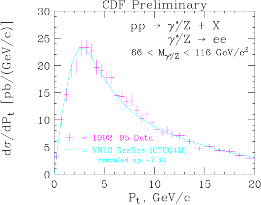
Figure 11: Transverse momentum distribution of the produced lepton pair in Drell-Yan production, $\bar{q}q\rightarrow\gamma^{*}/Z\rightarrow e^{+}e^{-}$, as measured by the CDF Collaboration at the Tevatron.

When trying to determine the kinematics of an event to better than some 10% ($={\cal O}(\alpha_{s})$), we need to take soft parton emission into account. One way to do this is to use transverse mass instead of transverse momentum of the lepton. For $W\rightarrow\ell\nu$ decay the transverse mass is defined as

$$m_{T}(\ell,{/\!\!\!\bf p}_{T})=\sqrt{(E_{T\ell}+{/\!\!\!E}_{T})^{2}-({\bf p}_{T\ell}+{/\!\!\!\bf p}_{T})^{2}}\;,$$ (46)

i.e. it is determined from the difference of squares of the transverse energy and the transverse momentum vector of the $\ell\nu$ pair. This is analogous to the definition of invariant mass, which in addition includes the contributions from the longitudinal momentum, along the beam axis. The transverse mass retains a Jacobian peak, at $m_{T}(\ell,{/\!\!\!\bf p}_{T})=m_{W}$, even in the presence of QCD radiation.

4.3 Extra $W$ and $Z$ bosons

The SM is a gauge theory based on the gauge group $G_{SM}=SU(3)\times SU(2)_{L}\times U(1)_{Y}$ and each of these factors is associated with a set of gauge bosons, the eight gluons of $SU(3)$, the photon and the $W^{\pm}$ and $Z$ of the electroweak sector. It is possible, however, that the gauge symmetry of nature is larger, which in turn would predict the existence of extra gauge bosons. The apparent symmetry of the SM would arise because the extra gauge bosons are too heavy to have been observed as yet, made massive by the spontaneous breaking of the extra gauge symmetry. Examples of such extended gauge sectors are left-right symmetric models [28] with

$$G=SU(3)\times SU(2)_{R}\times SU(2)_{L}\times U(1)_{B-L}\;,$$ (47)

where the new $SU(2)_{R}$ factor gives rise to an extra charged $W^{\prime}$ with $V+A$ couplings to quarks and leptons and an additional $Z^{\prime}$, or extensions with extra $U(1)$ factors,[4, 29]

$$G=SU(3)\times SU(2)_{L}\times U(1)\times U(1)\;,$$ (48)

which lead to the existence of an extra $Z^{\prime}$. Present indirect limits on such extra gauge bosons are relatively weak, and allow extra $W^{\prime}$ are $Z^{\prime}$ bosons to exist with masses above some 500 GeV.[30] These indirect bounds are obtained form the apparent absence of additional contact interactions, similar to Fermi’s four-fermion couplings, in low energy data. Given mass bounds of a few hundred GeV only, additional gauge bosons, with masses up to several TeV, could readily be observed at the LHC.

The cleanest method for discovering extra $Z^{\prime}$ bosons would be through a repetition of the historic CERN experiments [27] which lead to the discovery of the $Z$ in 1983, i.e. by searching for the $Z^{\prime}$ resonance peak in

$$\bar{q}q\rightarrow Z^{\prime}\rightarrow\ell^{+}\ell^{-}\;,\qquad\ell=e,\mu\;.$$ (49)

The reach of this search depends on the coupling $g^{\prime f}_{L,R}$ of the extra $Z^{\prime}$ to left- and right-handed fermions. The production cross section is proportional to $(g^{\prime q}_{L})^{2}+(g^{\prime q}_{R})^{2}$. The decay branching fraction, $B(Z^{\prime}\rightarrow\ell^{+}\ell^{-})$, depends on the relative size of this combination of left- and right-handed couplings for lepton $\ell$ to the same combination, summed over all fermions. If the product of production cross section times leptonic branching ratio,

$$\sigma\cdot B=\sigma(pp\rightarrow Z^{\prime})\;B(Z^{\prime}\rightarrow\ell^{+}\ell^{-})\;,$$ (50)

is the same as for the SM $Z$-boson, scaled up to $Z^{\prime}$ mass, i.e. if the couplings of the $Z^{\prime}$ are SM-like, the LHC experiments can observe a $Z^{\prime}$ with a mass up to $m_{Z^{\prime}}=5$ TeV. Smaller (larger) couplings would decrease (increase) this reach, of course.[9]

While the LHC will not be capable of repeating the precision experiments of LEP/SLC, for a $Z^{\prime}$, a lot of additional information can be obtained by more detailed observations of leptonic $Z^{\prime}$ decays.[29] One measurement which would be of particular importance is the determination of the lepton charge asymmetry. At the parton level, the forward-backward charge asymmetry measures the relative number of $\bar{q}q\rightarrow Z^{\prime}\rightarrow\ell^{+}\ell^{-}$ events where the $\ell^{-}$ goes into the same hemisphere as the incident quark, as compared to events where the $\ell^{+}$ goes into the quark direction. In terms of the pseudo-rapidity of the $\ell^{-}$, $\eta^{*}$, as measured relative to the incident quark direction, i.e.

$$\eta^{*}={1\over 2}\log{1+\cos\theta^{*}\over 1-\cos\theta^{*}}\;,$$ (51)

where $\theta^{*}$ is the c.m. frame angle between the incident quark and the final state $\ell^{-}$ (or the angle between the incident anti-quark and the final state $\ell^{+}$), the forward-backward asymmetry, at the parton level, is given by

$$\hat{A}_{FB}^{\ell}={\hat{\sigma}(\eta^{*}>0)-\hat{\sigma}(\eta^{*}<0)\over\hat{\sigma}(\eta^{*}>0)+\hat{\sigma}(\eta^{*}<0)}={3\over 4}\,{(g^{\prime q}_{R})^{2}-(g^{\prime q}_{L})^{2}\over(g^{\prime q}_{R})^{2}+(g^{\prime q}_{L})^{2}}\;{(g^{\prime\ell}_{R})^{2}-(g^{\prime\ell}_{L})^{2}\over(g^{\prime\ell}_{R})^{2}+(g^{\prime\ell}_{L})^{2}}$$ (52)

One sees that a measurement of the forward-backward asymmetry gives a direct comparison of left-handed and right-handed couplings of the $Z^{\prime}$ to leptons and quarks.

Unfortunately, at a $pp$-collider, the two proton beams have equal probabilities to originate the quark or the antiquark in the collision, and, therefore, the forward backward asymmetry averages to zero when considering all events. One can make use of the different Feynman $x$ distributions of up and down quarks as opposed to anti-quarks, however. At small $x$, quarks and anti-quarks have roughly equal pdf’s, $q(x)\approx\bar{q}(x)$, while at large $x$ the valence quarks dominate by a sizable fraction, $q(x)\gg\bar{q}(x)$. In the experiment one measures the rapidities $y_{+}$ and $y_{-}$ of the $\ell^{+}$ and $\ell^{-}$, respectively. Since the leptons are back-to-back in the c.m. frame, their c.m. rapidities cancel, and the sum of the lab frame rapidities gives the rapidity $y=y_{c.m.}$ of the c.m. frame,

$$y={1\over 2}(y_{+}+y_{-})={1\over 2}\log{x_{1}\over x_{2}}\;,$$ (53)

while their difference measures $\eta^{*}$,

$$\eta^{*}={1\over 2}\log{1+\cos\theta^{*}\over 1-\cos\theta^{*}}={1\over 2}(y_{-}-y_{+})\;.$$ (54)

At $y>0$ we have $x_{1}>x_{2}$, and therefore it is more likely that the quark came from the left, while at $y<0$ an anti-quark from the left is dominant. Measuring both $\eta^{*}$ and $y$, the charge asymmetry,

$$A(y)={{d\sigma\over dy}(\eta^{*}>0)-{d\sigma\over dy}(\eta^{*}<0)\over{d\sigma\over dy}(\eta^{*}>0)+{d\sigma\over dy}(\eta^{*}<0)}\;,$$ (55)

can be determined. Of course, we have $A(y)=-A(-y)$ at a $pp$ collider, where the two sides are equivalent, and the average over all $y$ vanishes. At fixed $y$, however, $A(y)$ is analogous to the forward-backward charge asymmetry at $e^{+}e^{-}$ colliders, and it measures the relative size of left-handed and right-handed $Z^{\prime}$ couplings.

Different extra gauge groups predict substantially different sizes for left- and right-handed couplings of the $Z^{\prime}$ to quarks and leptons. Thus, the lepton charge asymmetry, $A(y)$, is a very powerful tool to distinguish different models, once a $Z^{\prime}$ has been discovered.

Similar to the $Z^{\prime}$ search, the search for a heavy charged gauge boson, $W^{\prime}$, would repeat the $W$ search at CERN in the early eighties. One would study events consisting of a charged lepton and a neutrino, signified by missing transverse momentum opposite to the charged lepton direction. The mass of the $W^{\prime}$ is then determined by the Jacobian peak in the transverse mass distribution, at $m_{T}(\ell,{/\!\!\!\bf p}_{T})=m_{W^{\prime}}$. For a $W^{\prime}$ with SM strength couplings, the LHC can find it and measure its mass, up to $W^{\prime}$ masses of order 5 TeV, by searching for a shoulder in the transverse mass distribution and measuring its cutoff at $m_{W^{\prime}}$.[9]

4.4 Top search at the Tevatron

The leptonic decay of a $W$ or $Z$ produces a fairly clean signature at a hadron collider. Perhaps more typical for a new particle search was the discovery of the top quark [24, 25] at the Fermilab Tevatron. A much more complex signal needed to be isolated from large QCD backgrounds. At the same time the top discovery provides a beautiful example for the use of hadronic jets as a tool for discovering new particles. Let us have a brief, historical look at the top quark search at the Tevatron, from this particular viewpoint.

In $p\bar{p}$ collisions at the Tevatron, the top quark is produced via quark anti-quark annihilation, $q\bar{q}\rightarrow t\bar{t}$, and, less importantly, via $gg\rightarrow t\bar{t}$. Production cross sections have been calculated at next-to-leading order, and are expected to be around 5 pb for a top mass of 175 GeV.[31] The large top decay width which is expected in the SM,

$$\Gamma(t\rightarrow W^{+}b)\approx 1.6\;{\rm GeV}\;,$$ (56)

implies that the $t$ and $\bar{t}$ decay well before hadronization, and the same is true for the subsequent decay of the $W$ bosons. Thus, a parton level simulation for the complete decay chain, including final parton correlations, is a reliable means of predicting detailed properties of the signal. The top quark signal, $t\bar{t}\rightarrow bW^{+}\;\bar{b}W^{-}$, is determined by the various decay modes of the $W^{+}W^{-}$ pair, whose branching ratios were discussed in Sec. 3.1. In order to distinguish the signal from multi-jet backgrounds, the leptonic decay $W\rightarrow\ell\nu$ ($\ell=e,\;\mu$) of at least one of the two final state $W$s is extremely helpful. On the other hand, the leptonic decay of both $W$s into electrons or muons has a branching ratio of $\approx 4\%$ only, and thus the prime top search channel is the decay chain

$$t\bar{t}\;\rightarrow\;bW^{+}\;\bar{b}W^{-}\;\rightarrow\;\ell^{\pm}\nu\;q\bar{q}\;b\bar{b}\;.$$ (57)

Within the SM, this channel has an expected branching ratio of $\approx 30\%$. After hadronization each of the final state quarks in (57) may emerge as a hadronic jet, provided it carries enough energy. Thus the $t\bar{t}$ signal is expected in $W+3$ jet and $W+4$ jet events.

Figure 12: Number of $W+n$ jet events in the CDF top quark search as a function of jet multiplicity. Number of observed events are given without $b$-tagging (open circles) and with an SVX tag (triangles). The expected background, mainly from QCD $W+n$ jet events, is given by the cross-hatched bars. From the original CDF top quark discovery paper, Ref. [24].

Events with leptonic $W$ decays and several jets can also arise from QCD corrections to the basic Drell-Yan process $q\bar{q}\rightarrow W^{\pm}\rightarrow\ell^{\pm}\nu$. The process $ug\rightarrow dggW^{+}$, for example, will give rise to $W+3$ jet events and its cross section and the cross sections for all other subprocesses with a $W$ and three partons in the final state need to be calculated in order to assess the QCD background of $W+3$ jet events, at tree level. $W+n$ jet cross sections have been calculated for $n=3$ jets [32] and $n=4$ jets.[33] As in the experiment, the calculated $W+n$ jet cross sections depend critically on the minimal transverse energy of a jet. CDF, for example, requires a cluster of hadrons to carry $E_{T}>15$ GeV to be identified as a jet,[34] and this observed $E_{T}$ must then be translated into the corresponding parton transverse momentum in order to get a prediction for the $W+n$ jet cross sections.

At this level the QCD backgrounds are still too large to give a viable top quark signal. The situation was improved substantially by using the fact that two of the four final state partons in the signal are $b$-quarks, while only a small fraction of the $W+n$ parton background events have $b$-quarks in the final state. These fractions are readily calculated by using $W+n$ jet Monte Carlo programs. There are several experimental techniques to identify $b$-quark jets, all based on the weak decays of the produced $b$’s. One method is to use the finite $b$ lifetime of about $\tau=1.5$ ps which leads to $b$-decay vertices which are displaced by $\gamma c\tau=$ few mm from the primary interaction vertex. These displaced vertices can be resolved by precision tracking, with the aid of their Silicon VerteX detector in the case of CDF, and the method is, therefore, called SVX tag. In a second method, $b$ decays are identified by the soft leptons which arise in the weak decay chain $b\rightarrow W^{*}c,\;c\rightarrow W^{*}s$, where either one of the virtual $W$s may decay leptonically.[25, 34]

The combined results of using jet multiplicities and SVX $b$-tagging to isolate the top quark signal are shown in Fig. 12. A clear excess of $b$-tagged 3 and 4 jet events is observed above the expected background. The excess events would become insignificant if all jet multiplicities were combined or if no $b$-tag were used (see open circles). Thus jet counting and the identification of $b$-quark jets are critical for identification of top quark events.

Figure 13: Reconstructed mass distribution for $W+\geq 4$ jet events with a $b$-tag. The solid histogram represents the CDF data. Also included are the expected background (dotted histogram) and the expected signal+background for $m_{t}=175$ GeV. The insert shows the likelihood fit to determine the top quark mass, which yielded $m_{t}=176\pm 8\pm 10$ GeV at the time. From Ref. [24].

Beyond counting the number of jets above a certain transverse energy, the more detailed kinematic distributions, their summed scalar $E_{T}$’s [25] and multi-jet invariant masses, have also been critical in the top quark search. The top quark mass determination, for example, relies on a good understanding of these distributions. Ideally, in a $t\bar{t}\rightarrow(\ell^{+}\nu b)(q\bar{q}\bar{b})$ event, for example, the two subsystem invariant masses should be equal to the top quark mass,

$$m_{t}\approx m(\ell^{+}\nu b)\approx m(q\bar{q}\bar{b})\;.$$ (58)

Including measurement errors, wrong assignment of observed jets to the two clusters, etc. one needs to perform a constrained fit to extract $m_{t}$. The 1995 CDF result of this fit [24] is shown in Fig. 13. In addition, the figure demonstrates that the observed $b$-tagged $W+4$ jet events (solid histogram) are considerably harder than the QCD background (dotted histogram). On the other hand the data agree very well with the top quark hypothesis (dashed histogram).

By now, the top quark has been observed in all three decay channels of the $W^{+}W^{-}$ pair, purely leptonic $W$ decays, $W^{+}W^{-}\rightarrow\ell\nu jj$, and 4-jet decays, and all channels have been used to extract the top-quark mass. Results at present are

$$m_{t}=172.1\pm 7.1\;{\rm GeV}\;,$$ (59)

from the D0 Collaboration,[35] and

$$m_{t}=176.0\pm 6.5\;{\rm GeV}\;,$$ (60)

from the CDF Collaboration.[36]

5 Higgs search at the LHC

With the top-quark discovery at the Tevatron, the elementary fermions of the SM have all been observed. The missing ingredient, as far as the SM is concerned, is the Higgs boson. LEP2 is likely to find it if its mass is below $\approx 105$ GeV. The Tevatron has a chance to discover the Higgs boson in the processes $\bar{q}q\rightarrow WH,\;H\rightarrow\bar{b}b$ (for Higgs masses below $\approx 130$ GeV) [37] or $gg\rightarrow H\rightarrow WW^{*}$ (for 130 GeV$\mathrel{\raisebox{-2.58334pt}{$\stackrel{{\scriptstyle\textstyle<}}{{\sim}}$}}m_{H}\mathrel{\raisebox{-2.58334pt}{$\stackrel{{\scriptstyle\textstyle<}}{{\sim}}$}}180$ GeV) [38] if sufficient luminosity can be collected within the next few years. (Between 10 and 30 fb^-1 are required for this purpose.) The best candidate for Higgs discovery and detailed Higgs studies within the next ten years is the LHC, however.

Figure 14: Feynman graphs for the two dominant Higgs production processes at the LHC, (a) gluon-gluon fusion via a top-quark loop and (b) weak boson fusion.

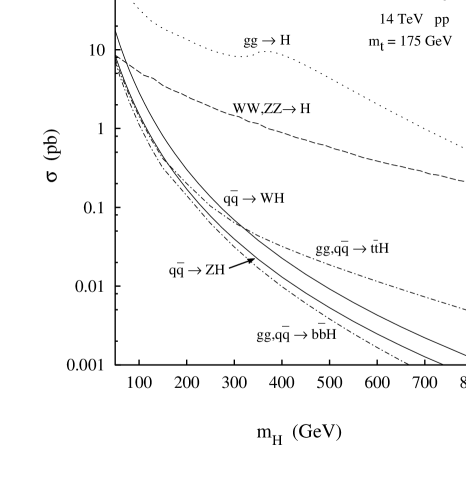
Figure 15: Production cross sections for the SM Higgs boson at the LHC. From Ref. [39].

5.1 Higgs production channels

A Higgs boson can be produced in a variety of processes at the LHC. The machine has sufficient energy to excite heavy quanta, and since the Higgs boson couples to other particles proportional to their mass, this leads to efficient Higgs production modes. The two dominant processes are shown in Fig. 14, gluon fusion, $gg\rightarrow H$, which proceeds via a top quark loop, and weak boson fusion, $qq\rightarrow qqH$, where the two incoming quarks radiate two virtual $W$s or $Z$s which then annihilate to form the Higgs. The expected cross sections for both are in the 1–30 pb range, and are shown in Fig. 15 as a function of the Higgs mass.

Beyond these two, a variety of heavy particle production processes may radiate a relatively light Higgs boson at an appreciable rate. These include $WH$ (or $ZH$) associated production,

$$\bar{q}q\rightarrow WH\;,$$ (61)

which is the analogue of $ZH$ production at $e^{+}e^{-}$ colliders, and $t\bar{t}H$ (or $b\bar{b}H$) associated production,

$$\bar{q}q\rightarrow\bar{t}tH\;,\qquad gg\rightarrow\bar{t}tH\;.$$ (62)

As can be seen in Fig. 15, these associated production cross sections are quite small for large Higgs boson masses, but can become interesting for $m_{H}\mathrel{\raisebox{-2.58334pt}{$\stackrel{{\scriptstyle\textstyle<}}{{\sim}}$}}150$ GeV, because the decay products of the additional $W$s or top quarks provide characteristic signatures of associated Higgs production events which allow for excellent background suppression.

In the most relevant region, 400 GeV $\mathrel{\raisebox{-2.58334pt}{$\stackrel{{\scriptstyle\textstyle>}}{{\sim}}$}}m_{H}\mathrel{\raisebox{-2.58334pt}{$\stackrel{{\scriptstyle\textstyle>}}{{\sim}}$}}110$ GeV, which will not be accessible by LEP, the total SM Higgs production cross section is of the order 10–30 pb, which corresponds to some $10^{5}$ events per year at the LHC, even at the initial ’low’ luminosity of ${\cal L}=10^{33}\;{\rm cm}^{-2}{\rm sec}^{-1}$. This already indicates that the main problem at the LHC is the visibility of the signal in an environment with very large QCD backgrounds, and this visibility critically depends on the decay mode of the Higgs. The decays $H\rightarrow b\bar{b},\;c\bar{c},\;gg$ all lead to a dijet signature and are very difficult to identify, because dijet production at a hadron collider is such a common-place occurrence. More promising are $H\rightarrow ZZ\rightarrow\ell^{+}\ell^{-}\ell^{+}\ell^{-}$ and $H\rightarrow\gamma\gamma$ which have much smaller backgrounds to contend with.

Figure 16: Decay branching fractions of the SM Higgs boson, as a function of Higgs mass. From Ref. [40].

5.2 Higgs search in the $H\rightarrow ZZ$ mode

The expected branching ratios of the SM Higgs to the various final states are shown in Fig. 16. For $m_{H}>180$ GeV, the $H\rightarrow ZZ$ threshold, Higgs decay to $WW$ and $ZZ$ dominates, and of the various decay modes of the two weak bosons, $ZZ\rightarrow\ell^{+}\ell^{-}\ell^{+}\ell^{-}$ gives the cleanest signature.[2] Not only can the invariant mass of the two lepton pairs be reconstructed, and their arising from $Z$ decay be confirmed, also the invariant mass of the four charged leptons reconstructs the Higgs mass. Thus, the Higgs signal appears as a resonance in the $m_{4\ell}$ invariant mass distribution. $ZZ$ backgrounds are limited at the LHC, they mostly arise from $\bar{q}q\rightarrow ZZ$ processes, i.e. continuum $ZZ$ production. The Higgs resonance needs to be observed on top of this irreducible background. Estimates are that with 100 fb^-1 the LHC detectors can see $ZZ\rightarrow 4\ell$ for 180 GeV$<m_{H}\mathrel{\raisebox{-2.58334pt}{$\stackrel{{\scriptstyle\textstyle<}}{{\sim}}$}}600$ GeV.[9, 10]

The only disadvantage of this ’gold-plated’ Higgs search mode is the relatively small branching ratio of $B(H\rightarrow ZZ\rightarrow\ell^{+}\ell^{-}\ell^{+}\ell^{-})\approx 0.15\%$. For large Higgs masses the gold-plated mode becomes rate limited, and additional Higgs decay modes must be searched for. $H\rightarrow ZZ\rightarrow\nu\bar{\nu}\ell^{+}\ell^{-}$, the ’silver-plated’ mode, has about a six times larger rate, but because of the unobserved neutrinos it does not provide for a direct Higgs mass reconstruction. The large missing $E_{T}$ and the two observed leptons allow a measurement of the transverse mass, however, with a Jacobian peak at $m_{H}$, analogous to the $W\rightarrow\ell\nu$ example. $H\rightarrow ZZ\rightarrow\nu\bar{\nu}\ell^{+}\ell^{-}$ events allow an extension of the Higgs search to $m_{H}\approx 0.8$–1 TeV.

Another promising search mode for a heavy Higgs boson is $H\rightarrow WW\rightarrow\ell\nu jj$, where the Higgs boson is produced in the weak boson fusion process, as depicted in Fig. 14(b). The two quarks in the process $qq\rightarrow qqH$ result in two additional jets, which have a large mutual invariant mass, and the presence of these two jets is a very characteristic signature of weak boson fusion processes. These two jets are typically emitted at forward angles, corresponding to pseudo-rapidities between $\pm 2$ to $\pm 4.5$. Requiring the observation of these two ’forward tagging jets’ substantially reduces the backgrounds and leads to an observable signal for Higgs boson masses in the 600 GeV to 1 TeV range and above.[9, 10, 41] This technique of forward jet-tagging can more generally be used to search for any weak boson scattering processes.[3, 42] However, it is as useful for the study of a weakly interacting Higgs sector at the LHC, and we shall consider it below in some detail in that context.

Fits to electroweak precision data, from LEP and SLC, from lower energy data as well as from the Tevatron, are increasingly pointing to a relatively small Higgs boson mass,[21] between 100 and 200 GeV, at least within the context of the SM. Thus, interest at present is focused on search strategies for a relatively light Higgs boson. The search in the gold-plated channel, $H\rightarrow\ell^{+}\ell^{-}\ell^{+}\ell^{-}$, can be extended well below the $Z$-pair threshold.[9, 10] As can be read off Fig. 16, the branching ratio $H\rightarrow ZZ^{*}$, into one real and one virtual $Z$, remains above the few percent level for Higgs boson masses as low as 130 GeV. With an integrated luminosity of around 100 fb^-1 the SM Higgs resonance can be observed the LHC, above $m_{H}\approx 130$ GeV. A problematic region is the 160 GeV$<m_{H}<$180 GeV range, however, where the branching ratio $H\rightarrow\ell^{+}\ell^{-}\ell^{+}\ell^{-}$ takes a serious dip: this is the region where the Higgs boson can decay into two on-shell $W$s, while the $ZZ$ channel is still below threshold for two on-shell $Z$s. While sufficiently large amounts of data will yield a positive Higgs signal in this region, the observation in the dominant decay channel, via $H\rightarrow W^{+}W^{-}\rightarrow\ell^{+}\nu\ell^{-}\bar{\nu}$ has a much higher rate and can in fact be distinguished from backgrounds as well.[43]

5.3 Search in the $H\rightarrow\gamma\gamma$ channel

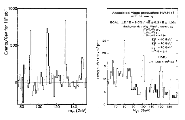
Figure 17: Expected $H\rightarrow\gamma\gamma$ signal in the CMS detector at the LHC, after one year of running at a luminosity of $10^{34}\;{\rm cm}^{-2}{\rm sec}^{-1}$. Shown are the expected Higgs resonance peaks in the $\gamma\gamma$ invariant mass distributions (a) in the inclusive $H\rightarrow\gamma\gamma$ search after background subtraction for Higgs masses of 90, 110, 130, and 150 GeV, and (b) for $WH$ and $\bar{t}tH$ associated production with $m_{H}=80$, 100, and 120 GeV. From Ref. [10].

For a relatively light SM Higgs boson, of mass $m_{H}\mathrel{\raisebox{-2.58334pt}{$\stackrel{{\scriptstyle\textstyle<}}{{\sim}}$}}150$ GeV, the cleanest search mode is the decay $H\rightarrow\gamma\gamma$. Photon energies can be measured with high precision at the LHC, resulting in a very good $m_{\gamma\gamma}$ invariant mass resolution, of order 1 GeV for Higgs masses around 100–150 GeV. In fact, the design of the LHC detectors has been driven by a good search capability for these events. Since the natural Higgs width is only a few MeV in this mass range, the Higgs would appear as as a very narrow peak in the $\gamma\gamma$ invariant mass distribution.

The simplest search is for all $H\rightarrow\gamma\gamma$ events, irrespective of the Higgs production mode. Backgrounds arise from double photon bremsstrahlung processes like

$$gq\rightarrow gq\gamma\gamma\;,\qquad qq\rightarrow qq\gamma\gamma\;,\quad{\rm etc.}$$ (63)

pair production of photons in $\bar{q}q$ annihilation and in gluon fusion (via quark loops),

$$\bar{q}q\rightarrow\gamma\gamma\;,\qquad\qquad gg\rightarrow\gamma\gamma\;,$$ (64)

and from reducible backgrounds, in particular from jets where the bulk of the jet’s energy is carried by a single $\pi^{0}$, whose decay into two nearby photons may not be resolved and may mimic a single photon in the detector.

Bremsstrahlung photons tend to be emitted close to the parent quark direction, i.e. they are close in angle to a nearby jet. The same is true for photons from $\pi^{0}$ decays, these photons are usually embedded into a hadronic jet. One therefore requires the signal photons to be well isolated, i.e. to have little hadronic activity at small angular separations

$$\Delta R=\sqrt{(\eta_{\gamma}-\eta_{j})^{2}+(\phi_{\gamma}-\phi_{j})^{2}}\;.$$ (65)

Here $(\eta_{\gamma},\;\phi_{\gamma})$ give the photon direction and $(\eta_{j},\;\phi_{j})$ denotes the direction of hadronic activity, be it hadrons, partons in a perturbative calculation, or jets. A practical requirement may be that the total energy carried by hadrons within a cone of radius $\Delta R=0.3$ be less that 10% of the photon energy and that no hard jet is found with a separation $\Delta R<0.7$. Photon isolation requirements drastically reduce bremsstrahlung and QCD ($\pi^{0}$) backgrounds and are absolutely crucial for identifying any signal.

Another characteristic feature of the backgrounds is their soft photon spectrum: background rates drop quite fast with increased photon transverse momentum, $p_{T\gamma}$. This plays into the features of the signal. Since a Higgs boson decays isotropically, with $E_{\gamma}=m_{H}/2$ in the Higgs rest frame, photon transverse momenta in the range $m_{H}/4\mathrel{\raisebox{-2.58334pt}{$\stackrel{{\scriptstyle\textstyle<}}{{\sim}}$}}p_{T\gamma}\leq m_{H}/2$ are favored. In practice, when searching for a Higgs boson in the 100 GeV $<m_{H}<$ 150 GeV range, one requires $p_{T\gamma_{1}}>40$ GeV, $p_{T\gamma_{2}}>25$ GeV for the two photons, which together with the isolation requirement reduces the background to a level of order $d\sigma/dm_{\gamma\gamma}=$100–200 fb/GeV.[10] This needs to be compared to the SM Higgs signal, which has a cross section, after cuts, of $\sigma\cdot B(H\rightarrow\gamma\gamma)\approx 40$ fb for masses around $m_{H}=120$ GeV.

The visibility of the signal crucially depends on the mass resolution of of the detector. For CMS (ATLAS) one expects a resolution of order $\sigma_{m}=\pm 0.8$ GeV ($\pm 1.5$ GeV). Taking the better CMS resolution and an integrated luminosity of 50 fb^-1 as an example, one would see $S=0.683\cdot 2000=1400$ signal events in a mass bin of full width 1.6 GeV, on top of a background of $B=13000\cdot 1.6=21000$ events, giving a statistical significance $S/\sqrt{B}$ of almost 10 standard deviations, a very significant discovery! The expected two-photon mass spectrum, after background subtraction, is shown in Fig. 17(a). The above example only conveys the rough size of the signal and background in the inclusive $H\rightarrow\gamma\gamma$ search. More detailed estimates for a range of Higgs masses, including detection efficiencies, the decline of background rates with increasing $m_{\gamma\gamma}$, and variations in the signal rate as a function of $m_{H}$ can be found in Refs. [9, 10].

The main disadvantage of the inclusive $H\rightarrow\gamma\gamma$ search is the relatively small signal size as compared to the background, $S:B\approx 1:15$ for CMS and even smaller for ATLAS. A much cleaner signal can be found by looking for Higgs production in association with other particles, in particular the isolated leptons arising from $W$ decays in $WH$ and $\bar{t}tH$ associated production. A high $p_{T}$ isolated lepton is very unlikely to be produced in most background processes with two photons, and, thus, a signal to background ratio of about 1:1 or even better can be achieved. The results of a simulation of the anticipated $m_{\gamma\gamma}$ spectrum are shown in Fig. 17(b), again for the CMS detector.[10] While $S:B$ is very good, cross sections are much lower than in the inclusive $H\rightarrow\gamma\gamma$ search and integrated luminosities of order 100 fb^-1 or larger are needed for a significant signal in these associated production channels.

5.4 Weak boson fusion

There is a danger in relying too much on the $H\rightarrow\gamma\gamma$ decay channel for a light Higgs boson, of course: it implicitly assumes that the Higgs partial decay widths are indeed as large as predicted by the SM. Approximately, the two-photon branching ratio is given by

$$B(H\rightarrow\gamma\gamma)={\Gamma(H\rightarrow\gamma\gamma)\over\Gamma(H\rightarrow\bar{b}b)+\dots}\;,$$ (66)

i.e. a strongly increased partial width for $H\rightarrow\bar{b}b$ can render the $H\rightarrow\gamma\gamma$ channel unobservably small. This is what happens in the MSSM, with its two Higgs doublets, which lead to two CP-even scalars, the light $h$ and a heavier state, $H$. For large $\tan\beta=v_{1}/v_{2}$, the $b$-quark Yukawa coupling is enhanced, leading to a suppressed $h\rightarrow\gamma\gamma$ branching ratio over large regions of parameter space. One thus needs to prepare for a search in other decay channels as well. And even if the $H\rightarrow\gamma\gamma$ mode is observed first, the other channels will be needed to learn about the various couplings of the Higgs boson, to weak bosons, quarks and leptons, i.e. they need to be studied in order to understand the dynamics of the symmetry breaking sector.

In any model which treats lepton and quark mass-generation symmetrically, the $H\rightarrow\bar{b}b$ and $H\rightarrow\tau^{+}\tau^{-}$ decay widths move in unison because both represent the isospin $-1/2$ component of a third generation doublet. Thus, the $h\rightarrow\tau^{+}\tau^{-}$ branching ratio is fairly stable, staying at the 8–9% level in e.g. the MSSM over large regions of parameter space where the $h\rightarrow\gamma\gamma$ branching ratio may be suppressed by large factors. Interestingly, the tau decay mode is observable in the most copious of the associated Higgs production processes, weak boson fusion as depicted in Fig. 14.

Traditionally, weak boson fusion has been considered mainly as a method for studying a strongly interacting symmetry breaking sector,[2] where one encounters either a very heavy Higgs boson or non-Higgs dynamics such as in technicolor models. However, as is evident from Fig. 15, the weak boson fusion cross section, $\sigma(qq\rightarrow qqH)$, is as large as a few pb also for a Higgs boson in the 100 GeV range, which in the SM corresponds to 10–20% of the total Higgs production rate.

A characteristic feature of weak boson fusion events are the two accompanying quarks (or anti-quarks) from which the “incoming” $W$s or $Z$s have been radiated (see Fig. 14(b)). In general these scattered quarks will give rise to hadronic jets. By tagging them, i.e. by requiring that they are observed in the detector, one obtains a powerful background rejection tool.[44, 45] Whether such an approach can be successful depends on the properties of the tagging jets: their typical transverse momenta, their energies, and their angular distributions.

Similar to the emission of virtual photons from a high energy electron beam, the incoming weak bosons tend to carry a small fraction of the incoming parton energy. At the same time the incoming weak bosons must carry substantial energy, of order $m_{H}/2$, in order to produce the Higgs boson. Thus the final state quarks in $qq\rightarrow qqH$ events typically carry very high energies, of order 1 TeV. This is to be contrasted with their transverse momenta, which are of order $p_{T}\approx m_{W}$. This low scale is set by the weak boson propagators in Fig. 14(b), which introduce a factor

$$D_{V}(q^{2})={-1\over q^{2}-m_{V}^{2}}\approx{1\over p_{T}^{2}+m_{V}^{2}}$$ (67)

into the production amplitudes and suppress the $qq\rightarrow qqH$ cross section for quark transverse momenta above $m_{V}$. The modest transverse momentum and high energy of the scattered quark corresponds to a small scattering angle, typically in the $1<\eta<5$ pseudo-rapidity region.

Figure 18: Transverse momentum and pseudo-rapidity distributions of the two (anti)quark jets in $qq\rightarrow qqH$ events at the LHC. Shown are (a) $d\sigma/dp_{Tj}$ for the highest (dashed curve) and lowest $p_{T}$ jet (solid curve) and (b) $d\sigma/d|\eta_{j}|$ for the most forward (dashed curve) and the most central jet (solid curve).

These general arguments are confirmed by Fig. 18, where the transverse momentum and pseudo-rapidity distributions of the two potential tagging jets are shown for the production of a $m_{H}=120$ GeV Higgs boson at the LHC. One finds that one of the two quark jets has substantially lower median $p_{T}$ ($\approx 35$ GeV) than the other ($\approx 70$ GeV), and therefore experiments must be prepared to identify fairly low $p_{T}$ forward jets. A typical requirement would be [48]

$$p_{T_{j(1,2)}}\geq 40,20~{}{\rm GeV}\,,\qquad|\eta_{j}|\leq 5.0\,,\qquad m_{j1,j2}>1\;{\rm TeV}\;,$$ (68)

where, in addition, the tagging jets are required to be in opposite hemispheres, with the Higgs decay products between them.

While these requirements will suppress backgrounds substantially, the most crucial issue is identification of the $H\rightarrow\tau\tau$ decay products and the measurement of the $\tau^{+}\tau^{-}$ invariant mass. The $\tau$’s decay inside the beam pipe and only their decay products, an electron or muon in the case of leptonic decays, $\tau^{-}\rightarrow\ell^{-}\bar{\nu}_{\ell}\nu_{\tau}$, and an extremely narrow hadronic jet for $\tau^{\pm}\rightarrow h^{\pm}\nu_{\tau}$ ($h=\pi,\rho,a_{1}$) are seen inside the detector. The presence of a charged lepton, of $p_{T}>20$ GeV, is crucial in order to trigger on an $H\rightarrow\tau^{+}\tau^{-}$ event. Allowing the other $\tau$ to decay hadronically then yields the highest signal rate. Even though the hadronic $\tau$ decay is seen as a hadronic jet, this jet is not a typical QCD jet. Rather, the $\tau$-jet is extremely well collimated and it normally contains a single charged track only (so called 1-prong $\tau$ decay). An analysis by ATLAS [9, 46] has shown that hadronically decaying $\tau$’s, of $p_{T}>40$ GeV, can be identified with an efficiency of 26% while rejecting QCD jets at the 1:400 level.

At first sight the two or more missing neutrinos in $H\rightarrow\tau^{+}\tau^{-}$ decays seem to preclude a measurement of the $\tau^{+}\tau^{-}$ invariant mass. However, because of the small $\tau$ mass, the decay products of the $\tau^{+}$ or the $\tau^{-}$ all move in the same direction, i.e. the directions of the unobserved neutrinos are known. Their energy can be inferred by measuring the missing transverse momentum vector of the event. Denoting by $x_{\tau_{\ell}}$ and $x_{\tau_{h}}$ the fractions of the parent $\tau$ carried by the observed lepton and decay hadrons, the transverse momentum vectors are related by

$${/\!\!\!\bf p}_{T}=({1\over x_{\tau_{l}}}-1)\;{\bf p}_{T\ell}+({1\over x_{\tau_{h}}}-1)\;{\bf p}_{Th}\;.$$ (69)

As long as the the decay products are not back-to-back, Eq. (69) gives two conditions for $x_{\tau_{i}}$ and provides the $\tau$ momenta as ${\bf p}_{\ell}/x_{\tau_{l}}$ and ${\bf p}_{h}/x_{\tau_{h}}$, respectively. As a result, the $\tau^{+}\tau^{-}$ invariant mass can be reconstructed,[47] with an accuracy of order 10–15%.

Backgrounds to $H\rightarrow\tau\tau$ events in weak boson fusion arise from several sources. First is the production of real $\tau^{+}\tau^{-}$ pairs in “$Zjj$ events”, where the real or virtual $Z$ or photon, which decays into a $\tau$ pair, is produced in association with two jets. In addition, any source of isolated leptons and three or more jets gives a background since one of the jets may be misidentified as a $\tau$ hadronic decay. Such reducible backgrounds can arise from $W+3$ jet production or heavy flavor production, in particular $\bar{b}bjj$ events, where the $W$ or one of the $b$-quarks decay into a charged lepton. Identifying the two forward jets of the signal, with a large separation, $|\eta_{j_{1}}-\eta_{j_{2}}|>4.4$, and large invariant mass, substantially limits these backgrounds, as do the $\tau$-identification requirements. Additional background reduction is achieved by asking for consistent values of the reconstructed $\tau$ momentum fractions carried by the central lepton and $\tau$-like jet,

$$x_{\tau_{l}}<0.75\,,\qquad x_{\tau_{h}}<1\,.$$ (70)

Finally, a characteristic difference between the weak boson fusion signal and the QCD backgrounds is in the amount and angular distribution of gluon radiation in the central region.[49] The $qq\rightarrow qqH$ signal proceeds without color exchange between the scattered quarks. Similar to photon bremsstrahlung in Rutherford scattering, gluon radiation will be emitted in the very forward and very backward directions, between the tagging jets and the beam direction. Gluons giving rise to a soft jet are a rare occurrence in the central region. The background processes, on the other hand, proceed by color exchange between the incident partons, and here, fairly hard gluon radiation in the central region is quite common. A veto on any additional jet activity between the two tagging jets, of $p_{Tj}>20$ GeV, is expected to reduce the QCD backgrounds by about 80% while reducing the signal by 20-30% only.[48] Combining these various techniques, forward jet tagging, $\tau$-identification, $\tau$-pair mass reconstruction, and the central jet veto, one obtains a very low background signal (S:B $\approx$ 7:1 for $m_{H}=120$ GeV, significantly worse only for a Higgs which is degenerate with the $Z$) which is large enough to give a highly significant signal with an integrated luminosity of 30–50 fb^-1. The expected $\tau$-pair invariant mass distribution, for a Higgs mass of 120 GeV, is shown in Fig. 19.

Figure 19: Reconstructed $\tau^{+}\tau^{-}$ invariant mass distribution expected in weak boson fusion events at the LHC, for a SM Higgs boson of mass $m_{H}=120$ GeV. The solid line represents the sum of the signal and all backgrounds. Individual components are shown as histograms: the $qq\rightarrow qqH$ signal (solid), the irreducible QCD $Zjj$ background (dashed), the irreducible EW $Zjj$ background (dotted), and the combined $Wj+jj$ and $b\bar{b}jj$ reducible backgrounds (dash-dotted). From Ref. [48].

The forward jet tagging and central jet vetoing techniques described above can be used for isolating any weak boson fusion signal. Another example is the search for $H\rightarrow\gamma\gamma$ events, where the Higgs has been produced via $qq\rightarrow qqH$. About 20-30 fb^-1 of integrated luminosity are sufficient to observe the SM Higgs boson in the 110–150 GeV mass range this way,[50] which is comparable to the inclusive $H\rightarrow\gamma\gamma$ search described earlier. By observing both production channels, however, $gg\rightarrow H$ and $qq\rightarrow qqH$, separate information is obtained on the $H\bar{t}t$ and $HVV$ couplings which determine the production cross sections.

As should be clear from the preceding examples, a veritable arsenal of methods is available at the LHC to search for the Higgs boson and to analyze its properties. A single one of the methods may be sufficient for discovery of the Higgs and measurement of its mass. However, discovery will only start a much more important endeavor, for which all the tools will be needed: determining the various couplings of the Higgs boson to gauge bosons and heavy fermions, answering the question whether additional particles arise from the symmetry breaking sector, like the $H^{\pm}$ and pseudo-scalar $A$ of two Higgs doublet models, and, thus, finding the dynamics which is responsible for $SU(2)\times U(1)$ breaking in nature. New methods are still being developed for this purpose, and all will be needed to answer these fundamental questions.

6 Conclusions

Our discussion has touched on a number of the investigations which can be conducted at $e^{+}e^{-}$ and hadron colliders, or at a future muon collider. It is by no means complete, however. The strategies for identifying a supersymmetry signal at the LHC, for example, have not been discussed in any detail. The reader is referred to other TASI lectures for this purpose.[5] Some general properties of experimental possibilities should have emerged, however. Both $e^{+}e^{-}$ and hadron colliders provide the necessary energy and luminosity to search for new particles, and to investigate their properties, once they have been discovered. In these goals, the two types of machines complement each other.

For the foreseeable future, hadron colliders produce the highest parton center of mass energies and therefore have the longest reach in producing very heavy objects. Their disadvantage is the large $pp$ cross section, i.e. the fact that any new physics signal needs to be extracted from backgrounds whose rates are larger by many orders of magnitude. We have studied several examples of how this can be done. Electroweak decays, with their resulting isolated photons and leptons, are crucial to identify top quarks, heavy gauge bosons or the Higgs. But precise features of the hadronic part of new particle production events provide equally important information. Examples are the multiple jets and tagged $b$-quarks in top decays, and the two forward tagging jets in weak boson fusion events.

$e^{+}e^{-}$ colliders benefit from much better signal to background ratios, lack of an underlying event as encountered in hadron collisions, and the constrained kinematics which results from the point-like character of the beam particles: beam constraints are extremely useful tools in the reconstruction of events. The disadvantage of $e^{+}e^{-}$ colliders is their limited energy reach, of course, as compared to hadron colliders.

Only time will show which of these machines, the Tevatron, LEP2, the LHC, an NLC, or a muon collider, will give us the most important clues to what lies beyond the standard model. But given their capabilities, exciting times ahead of us are virtually assured.

References

References

- [1] For a full discussion see the lectures of G. Altarelli, these proceedings [hep-ph/9811456].
- [2] See e.g. J. F. Gunion, H. E. Haber, G. Kane, and S. Dawson, The Higgs Hunter’s Guide, Addison-Wesley (1990).
- [3] M. E. Peskin, Beyond the Standard Model, Lectures given at The 1996 European School of High-Energy Physics, SLAC-PUB-7479 (1997) [hep-ph/9705479].
- [4] For details and further references see M. Cvetic, these proceedings.
- [5] See the lectures by N. Polonsky, these proceedings; Xerxes Tata, Supersymmetry: Where it is and how to find it, in TASI 95, QCD and Beyond, ed. by D.E. Soper, World Scientific (1996), p. 163 [hep-ph/9510287].
- [6] For recent reviews see V. Barger, preprint MADPH-98-1040 (1998) [hep-ph/9803480]; J.F. Gunion, preprint UCD-98-5 (1998) [hep-ph/9802258]; V. Barger et al., The physics capabilities of colliders, in Santa Barbara 1996, Future high energy colliders, p. 219 [hep-ph/9704290].
- [7] See e.g. V. Barger and R. Phillips, Collider Physics, Addison-Wesley (1987); R.K. Ellis, W.J. Stirling and B.R. Webber, QCD and Collider Physics, Cambridge Univ. Press (1996).
- [8] E. Keil, in Proceedings of the ECFA Workshop on LEP 200, ed. by A. Böhm and W. Hoogland, report CERN 87-08 (1987), Vol. I, p. 17.
- [9] W. W. Armstrong et al., Atlas Technical Proposal, report CERN/LHCC/94-43 (1994).
- [10] G. L. Bayatian et al., CMS Technical Proposal, report CERN/LHCC/94-38 (1994).
- [11] K. Hagiwara, K. Hikasa, R.D. Peccei and D. Zeppenfeld, Nucl. Phys. B282, 253 (1987).
- [12] W. Beenakker et al., cross sections and distributions, in Physics at LEP2, ed. by G. Altarelli, T. Sjöstrand and F. Zwirner, CERN Yellow report CERN-96-01 (1996) vol. 1, p. 79 [hep-ph/9602351] and references therein.
- [13] G. Gounaris et al., Triple gauge boson couplings, in Physics at LEP2, ed. by G. Altarelli, T. Sjöstrand and F. Zwirner, CERN Yellow report CERN-96-01 (1996) vol. 1, p. 525 [hep-ph/9601233].
- [14] ADLO and D0 TGC Combination Group, report LEPEWWG/TGC/98-02, summer 1998.
- [15] Z. Kunszt et al., Determination of the mass of the boson, in Physics at LEP2, ed. by G. Altarelli, T. Sjöstrand and F. Zwirner, CERN Yellow report CERN-96-01 (1996) vol. 1, p. 141 [hep-ph/9602352].
- [16] LEP Electroweak Working Group, LEP WW cross section and W mass for ’98 summer conferences, report LEPEWWG/MW/98-02 at http://www.cern.ch/LEPEWWG/wmass/.
- [17] CDF Collaboration, F. Abe et al., Phys. Rev. Lett. 75, 11 (1995); D0 Collaboration, B. Abbot et al., Phys. Rev. Lett. 80, 3000 (1998).
- [18] For details see G.F Giudice et al., Searches for new physics, in Physics at LEP2, ed. by G. Altarelli, T. Sjöstrand and F. Zwirner, CERN Yellow report CERN-96-01 (1996) vol. 1, p. 463 [hep-ph/9602207] and references therein.
- [19] P. Rebecchi, talk given at ICHEP98, Vancouver, Canada, July 23-29, 1998.
- [20] J. Erler and P. Langacker, to appear in the Proceedings of the 5th International WEIN Symposium, Santa Fe, NM, June 14-21, 1998 [hep-ph/9809352].
- [21] For a recent summary see W. Marciano, talk given at the 1999 DPF meeting, Los Angeles, Jan.5–9, 1999.
- [22] M. Carena et al., Higgs Physics, in Physics at LEP2, ed. by G. Altarelli, T. Sjöstrand and F. Zwirner, CERN Yellow report CERN-96-01 (1996) vol. 1, p. 351 [hep-ph/9602250] and references therein.
- [23] For recent reviews of physics at linear colliders see e.g. E. Accomando et al., Phys. Rept. 299, 1 (1998) [hep-ph/9705442]; S. Kuhlman et al., Physics and Technology of the NLC, report SLAC-R-0485 (1996) [hep-ex/9605011].
- [24] CDF Collaboration, F. Abe et al., Phys. Rev. Lett. 74, 2626 (1995).
- [25] D0 Collaboration, S. Abachi et al., Phys. Rev. Lett. 74, 2422 (1995); Phys. Rev. Lett. 74, 2632 (1995); Phys. Rev. D52, 4877 (1995).
- [26] See e.g. H.L. Lai et al., Phys. Rev. D55, 1280 (1997); A.D. Martin, R.G. Roberts, W.J. Stirling, and R.S. Thorne, Eur. Phys. J. C4, 463 (1998).
- [27] UA1 Collaboration, G. Arnison et al., Phys. Lett. 122B, 103 (1983); UA2 Collaboration, M. Banner et al., Phys. Lett. 122B, 476 (1983).
- [28] D. Chang, R. Mohapatra, and M. Parida, Phys. Rev. Lett. 50, 1072 (1984); Phys. Rev. D30, 1052 (1984).
- [29] For a recent review see e.g. M. Cvetic and P. Langacker, preprint hep-ph/9707451, to appear in Perspectives in Supersymmetry, World Scientific, ed. by G. Kane.
- [30] G.-C. Cho, K. Hagiwara, and S. Matsumoto, Eur. Phys J. C5, 155 (1998) [hep-ph/9707334]; G.-C. Cho, K. Hagiwara, and Y. Umeda, hep-ph/9805448.
- [31] P. Nason, S. Dawson, and R. K. Ellis, Nucl.Phys. B303, 607 (1988); E. Laenen, J. Smith, and W. L. van Neerven, Nucl.Phys. B369, 543 (1992); Phys. Lett. B321, 254 (1994); E. Berger and H. Contopanagos, Phys. Rev. D54, 3085 (1996); S. Catani et al., Phys. Lett. B378, 329 (1996).
- [32] V. Barger, T. Han, J. Ohnemus, and D. Zeppenfeld, Phys. Rev. D40, 2888 (1989); F. A. Berends, W. T. Giele, and H. Kuijf, Nucl. Phys. B321, 39 (1989); F. A. Berends et al., Phys. Lett. B224, 237 (1989).
- [33] F. A. Berends, H. Kuijf, B. Tausk, and W. T. Giele, Nucl. Phys. B357, 32 (1991).
- [34] CDF Collaboration, F. Abe et al., Phys. Rev. D50, 2966 (1994); Phys. Rev. D52, 2605 (1995).
- [35] D0 Collaboration, B. Abbot et al., report FERMILAB-PUB-98-261-E (1998), [hep-ex/9808029].
- [36] CDF Collaboration, F. Abe et al., Phys. Rev. Lett. 82, 271 (1999).
- [37] S. Kim, S. Kuhlmann, and W.M. Yao, report CDF-ANAL-EXOTIC-PUBLIC-3904 (1996), presented at 1996 DPF/DPB Summer Study on New Directions for High-energy Physics (Snowmass 96), Snowmass, CO, 25 Jun - 12 Jul 1996.
- [38] Tao Han and Ren-Jie Zhang, Phys. Rev. Lett. 82, 25 (1999) [hep-ph/9807424].
- [39] J. F. Gunion, A. Stange, and S. S. D. Willenbrock, in Electroweak symmetry breaking and new physics at the TeV scale, ed. by T.L.Barklow et al., p. 23-145 [hep-ph/9602238].
- [40] M. Spira and P. Zerwas, Electroweak symmetry breaking and Higgs Physics, in Schladming 1997 Computing particle properties, p. 161-225, [hep-ph/9803257].
- [41] K. Iordanidis and D. Zeppenfeld, Phys. Rev. D57, 3072 (1998), [hep-ph/9709506].
- [42] J. Bagger et al., Phys. Rev. D49, 1246 (1994); Phys. Rev. D52, 3878 (1995).
- [43] M. Dittmar and H. Dreiner, Phys. Rev. D55, 167 (1997) [hep-ph/9608317].
- [44] R. N. Cahn et al., Phys. Rev. D35, 1626 (1987); V. Barger et al., Phys. Rev. D37, 2005 (1988); R. Kleiss and W. J. Stirling, Phys. Lett. 200B, 193 (1988).
- [45] U. Baur and E. W. N. Glover, Nucl. Phys. B347, 12 (1990); U. Baur and E. W. N. Glover, Phys. Lett. B252, 683 (1990); D. Froideveaux, in Proceedings of the ECFA Large Hadron Collider Workshop, Aachen, Germany, 1990, edited by G. Jarlskog and D. Rein (CERN report 90-10, Geneva, Switzerland, 1990), Vol II, p. 444; M. H. Seymour, ibid, p. 557; V. Barger, K. Cheung, T. Han, J. Ohnemus, and D. Zeppenfeld, Phys. Rev. D44, 1426 (1991).
- [46] D. Cavalli et al., ATLAS Internal Note PHYS-NO-051, Dec. 1994.
- [47] R. K. Ellis et al., Nucl. Phys. B297, 221 (1988).
- [48] D. Rainwater, D. Zeppenfeld, and K. Hagiwara, Phys. Rev. D59 (1999) 014037.
- [49] Y. L. Dokshitzer, V. A. Khoze, and S. Troyan, in Proceedings of the 6th International Conference on Physics in Collisions, (1986) ed. M. Derrick (World Scientific, Singapore, 1987) p. 365; J. D. Bjorken, Int. J. Mod. Phys. A7, 4189 (1992); Phys. Rev. D47, 101 (1993); J. D. Bjorken, in Proceedings of the International Workshop on Photon-Photon Collisions, (1992) ed. D. O. Caldwell and H. P. Paar (World Scientific, Singapore, 1992) p. 502.
- [50] D. Rainwater and D. Zeppenfeld, J. High Energy Physics 12 (1997) 005.