QCD and Nuclear Physics,

Abstract

The main part of this talk is a review and summary of how QCD is used in two main areas of nuclear physics, namely in determining the quark flavor and spin content of the proton and in ultrarelativistic heavy ion collisions. Brief comments are made concerning effective theories in hadron physics and on the separation of various twists in using the operator product expansion to analyze hard processes.

1 Introduction

Quantum Chromodynamics (QCD) is a fundamental theory in the sense that one expects QCD to exist not just as a perturbative expansion but also in its strong coupling regime. There is good evidence from lattice QCD calculations that this is indeed the case. QCD stands in contrast to QED or the Electroweak Theory which have good perturbative expansions but which are not expected to exist in the strong coupling regime. In particular it is widely believed that the Electroweak Theory must be unified with additional interactions at a scale below its Landau ghost.

The likelihood that only asymptotically free theories make sense puts severe restrictions on the use of “effective” field theories, field theories that are to be used in a limited range of scales. For example, it probably does not make much sense to try and describe low energy pion-nucleon interactions in terms of a pseudoscalar meson-nucleon interaction Lagrangian since the coupling necessary in such a description is so strong that the theory is internally inconsistent even at low energy scales. Of course the Born terms (tree graphs) of such a theory still make sense since they represent an analytic structure which is completely determined by the lowest lying states of the pion-nucleon system.

There is a special property of pion interactions which makes it possible to use particular effective theories as a description of low energy pion-nucleon interactions. That special property is chiral symmetry. One of the properties of the pion, as the Nambu-Goldstone boson of chiral symmetry breaking, is the fact that its couplings become weak at low momentum. Thus if one uses an effective chiral theory to describe low energy pion-nucleon interactions, and if a cutoff is introduced so that the couplings never grows large, then one can use that effective theory, even in a nonperturbative manner, to make precise calculations[1, 2, 3, 4, 5]. Such theories tend to have quite a few parameters since the cutoff is not very high and all the dynamics above the cutoff must be put into parameters of the effective theory. There has been much interest[1, 6] and progress in the last few years using effective theories to describe light nuclei in terms of pion-pion and pion-nucleon interactions. It is perhaps a bit too early to decide whether this description is superior to the traditional potential approach, but one can hope to get better insight as to where it is more useful to use quarks and gluons to describe hadronic physics and where it is better to use effective degrees of freedom.

As far as is known QCD-type theories are the only four-dimensional field theories “known” to exist as fundamental theories. The goal in strong interaction physics is to understand how QCD works. Few physicists doubt the validity of QCD as the theory of the strong interactions. However, QCD is a rich and sophisticated theory about which there is still much to understand and appreciate.

I shall cover three topics in this talk. Firstly, I shall review progress in understanding the quark and gluon structure of the proton wavefunction. This has become one of the most active fields in nuclear physics in which the Jefferson Laboratory has now begun to make important new contributions. This part of my talk will have some overlap with and is complementary to the talks of L. Cardman[7] and A. Magnon][8]. The next topic to be covered is that of heavy ion collisions and small-x physics. The object here is to describe the relationships between the physics being pursued in high energy small-x physics and that which will become available at heavy ion colliders at Brookhaven and at CERN. The final topic is perhaps more of a remark, but it is a remark which is important for medium energy physics. The point is that the separation between perturbative and nonperturbative QCD is not always so easy to define. Nevertheless, one must often make such a separation in medium energy phenomenology and care must be taken to insure that that the separation, even if “scheme” dependent, is done consistently. A good example is a recent analysis by Kataev[9] and his collaborators of the description of the $F_{3}$ structure function in QCD.

2 Spin and Strangeness in the proton

2.1 Spin and the constituent quark model

In the constituent quark model the proton is made of two up-quarks and a down-quark. In the nonrelativistic version the three quarks are in zero orbital angular momentum states and so the spin of the proton is given by the sum of the spins of the quarks. With the usual SU(6) wavefunctions[10], and with $\Delta q$ labeling the z-component of spin of the quark $q$, one has

$$\Delta u=4/3,\Delta d=-1/3$$ (1)

leading to

$$G_{A}=\Delta u-\Delta d=5/3$$ (2)

and a total spin of the proton, $\Delta\Sigma$, given by

$$\Delta\Sigma=\Delta u+\Delta d=1.$$ (3)

The nonrelativistic quark model gives a reasonable picture of the proton but the value of $G_{A}$ is clearly somewhat high.

Relativistic quark models give better agreement with experiment for $G_{A}.$ Typically[11] one has

$$\Delta u\approx 1,\Delta d\approx-1/4$$ (4)

giving

$$G_{A}=\Delta u-\Delta d\approx 5/4$$ (5)

and

$$\Delta\Sigma=\Delta u+\Delta d\approx 3/4.$$ (6)

In neither the nonrelativistic nor in the relativistic versions of the model is there any room for strange quarks in the proton. In addition to $G_{A}$ the quark model gives a very good account of baryon magnetic moments and it has been the basis on which spectroscopy of mesons and baryons has been discussed for some time[10]. Much of what follows will be concerned with whether the quark model is able to give a reasonable account of the protons total spin.

2.2 How to measure spin

The axial vector current of flavor-f quarks is given by

$$j_{5\mu}^{f}=\tilde{q}_{f}\gamma_{\mu}\gamma_{5}q_{f}.$$ (7)

For free quarks

$$(ps|j_{5\mu}|ps)=2ms_{\mu}\mathrel{\longrightarrow\atop\to\infty}2\lambda p_{\mu}$$ (8)

where $s_{\mu}$ is the fermion spin four-vector corresponding to a quark with spin orientation $\vec{s}$ in its rest system, and where $\lambda$ is the quark helicity. In a frame where quarks have a large longitudinal momentum it is convenient to quantize spin along the direction of the large momentum.

In the quark-parton picture of the proton it is natural to suppose that

$$(Ps|j_{5\mu}^{f}|Ps)=2M_{P}s_{\mu}\Delta q_{f}$$ (9)

where $|Ps>$ is a proton state, and where $\Delta q_{f}$ is the fraction of the proton’s spin carried by quarks of flavor f.

In spin-dependent deep inelastic scattering on a proton one can measure a particular combinarning: Citation ‘Iof’ on page 3 undefined on input line 179. ! Missintion of axial vector current matrix elements, that given by

$$2Ms_{\mu}\int_{0}^{1}dx\ g_{1}^{P}(x,Q^{2})={1\over 2}\sum_{f}e_{f}^{2}(Ps|j_{5\mu}^{f}|Ps).$$ (10)

Scattering on neutrons gives an independent combination of axial vector currents. Defining

$$\int_{0}^{1}dxg_{1}^{P(N)}(x,Q^{2})=\Gamma_{1}^{P(N)}(Q^{2})$$ (11)

and using (9), one finds

$$\Gamma_{1}^{P}={1\over 2}({4\over 9}\Delta u+{1\over 9}\Delta d+{1\over 9}\Delta s)$$ (12)

and

$$\Gamma_{1}^{N}={1\over 2}({4\over 9}\Delta d+{1\over 9}\Delta u+{1\over 9}\Delta s).$$ (13)

An additional relation, involving $\Delta u,\Delta d$ and $\Delta s$ comes from semi- leptonic hyperon decays[12]. After using SU(3) flavor symmetry one finds

$$3F-D=\Delta u+\Delta d-2\Delta s.$$ (14)

Equations (12) - (14) apparently (but see below) give enough information to determine $\Delta q_{f}$ from $\Gamma_{1}^{P},\Gamma_{1}^{N},F$ and $D.$

2.3 Bare versus constituent quarks

In the constituent quark model the proton is described in terms of quarks which are not really point-like and which are not the quark degrees of freedom which appear in the QCD Lagrangian. The quark fields in (7) and (10) are the fundamental (bare) fields of the QCD Lagrangian. A basic assumption of the constituent quark model is that for static matrix elements one may replace the fundamental quark fields by the constituent (effective) quark fields of the quark model. This gives a method of calculating forward, or near forward, matrix elements of local bare quark currents in terms of wavefunctions of the constituent quark model. This is the basis on which one can see if there is agreement between the quark model and results obtained from deep inelastic scattering which do not directly measure constituent quarks but which, through relations like (10), do lead to static matrix elements of local currents.

2.4 A final subtlety

While (9) is a plausible assumption in fact it is not quite right. The correct relation is [13, 14, 15, 16]

$$(Ps|j_{5\mu}^{f}|Ps)=2Ms_{\mu}(\Delta q_{f}-{\alpha\over 2\pi}\Delta G)$$ (15)

with $\Delta G$ the amount of the proton’s spin carried by gluons. The argument for (15) is subtle and still not without controversy. I think the simplest argument for its validity comes from considering an example in quantum electrodynamics with massless electrons. At order $\alpha$ a virtual photon can break up into an electron-positron pair. Because helicity is conserved in electromagnetic interactions the helicities of the electron and positron will be of opposite sign. This if one takes the matrix element of $j_{5\mu}=\bar{\psi}\gamma_{\mu}\gamma_{5}\psi$ between virtual photon states, at order $\alpha,$ one would expect to get zero since $j_{5\mu},$ from (8), is supposed to measure electron (and positron) helicities. (The situation is illustrated in Fig.1.) However, the matrix element turns out to be $-{\alpha\over 2\pi},$ for a transversely polarized photon having helicity 1, despite the fact that any given electron-positron state gives a zero value. This is the axial anomaly and $-{\alpha\over 2\pi}$ is the value of the axial anomaly. In QCD exactly the same phenomenon occurs. The $-{\alpha\over 2\pi}$ in (15) is the anomaly value while $\Delta G$ gives the net helicity of gluons in the proton. The $-{\alpha\over 2\pi}$ comes from effects which cannot be ascribed to the quark wavefunction of the proton and is one of the most profound elements in QCD.

Figure 1: The axial vector current couples to electrons and positrons having opposite helicities

2.5 Results from spin-dependent deep inelastic scattering

There are several groups that have done extensive global fits, using a second order renormalization group formalism, to spin-dependent deep inelastic scattering[17, 18, 19]. The experimental situation is discussed in some detail in the talk of A. Magnon[8]. Here, I shall briefly recount the results found by Altarelli et al who have carried out a series of fits to all the available data. The effect of polarized gluons is quite important in the various fits. The preferred fit has

$$\Delta u=0.86,\Delta d = -0.37,\Delta s=-0.05$$ (16)

$$\Delta G = 1.4\pm 0.9$$

giving

$$\Delta\Sigma=0.44\pm 0.09.$$ (17)

While these numbers are not in perfect agreement with the relativistic quark model the situation is not so bad either. In particular, the reasonably small value for $\Delta s$ is much more comfortable for the quark model that were early values. However, because of the large errors on $\Delta G$ it is perhaps premature to take the final results as conclusive. The situation would be considerably improved by a direct measurement of $\Delta G,$ as planned at COMPASS and RHIC and which could also be done well at HERA. A few reliable points for $\Delta G(x,Q^{2})$ would help considerably to fix the first moment, $\Delta G,$ of $\Delta G(x,Q^{2}).$

2.6 Strangeness as viewed by vector currents

In the previous sections we have seen how spin-dependent deep inelastic scattering gives information on the polarized quark and gluon distributions of the proton. New experiments at Bates and the Jefferson Laboratory give complimentary information on the number of strange quarks in the proton. By measuring very accurately parity violating elastic electron-proton scattering information on the contribution of strange quarks to the proton’s electromagnetic form factors can be obtained. This is discussed in some detail in the talk of L. Cardman[7] so I will simply state the results here and then comment on their significance and how they fit in with the general program of determining the quark and gluon content of the proton. If $G_{E(M)}^{s}(Q^{2})$ stands for the strange quark contribution to the electric (magnetic) form factor of the proton at a momentum transfer $Q^{2}$ then the new result from the SAMPLE experiment at Bates is[20]

$$G_{M}^{s}(Q^{2}=0.1GeV^{2})=0.23\pm 0.37\pm 0.15\pm 0.19$$ (18)

where the first error is statistical, the second is a systematic error and the third is due to the axial form factor $G_{A}^{Z}.$ The HAPPEX experiment at the Jefferson Laboratory[21] finds

$$G_{E}^{s}+0.39\ G_{M}^{s}=0.023\pm 0.034\pm 0.022\pm 0.026$$ (19)

at $Q^{2}=0.47GeV^{2}$ where the first error is statistical, the second systematic and the third comes from uncertainties in the electric form factor of the neutron. To set the scale for these numbers we note that in the constituent quark model

$$G_{M}^{u}(0)=2.47,G_{M}^{d}(0)=0\cdot 32$$ (20)

and

$$G_{E}^{u}(0)=4/3,G_{E}^{d}(0)=-1/3$$ (21)

give the up and down contributions to the proton’s magnetic moment and charge, respectively.

The HAPPEX result suggests that strange quarks give no more than a few percent of the up plus down contribution to $G_{E}+0.39G_{M}.$ The SAMPLE result is also consistent with a small strange quark contribution, but the limit is perhaps not too stringent.

2.7 Summary on quark content of the proton

Perhaps the main issue in determining the quark and gluon content of the proton is the issue of how many and “what kind” of strange quarks are to be found in the proton’s wavefunction. At first sight this would seem to be a simple problem whose answer, at least roughly, has been known for some time. After all, spin-independent deep inelastic lepton-proton experiments have determined that $x(s(x,Q^{2})+\bar{s}(x,Q^{2}))$ is sizeable. Indeed, the strange quark sea is about one-half that of the non-strange sea.

However, a moment’s reflection is enough to realize that while it is interesting to know the number, and the Bjorken  x  distribution, of strange quarks in the proton it is even more important to know if those strange quarks are just short time fluctuations which play no role in the dynamics of the proton or if the strange quarks live long enough to be essential in determining the proton’s mass and wavefunction. For example, the fluctuation of a gluon of the proton into an $s\bar{s}$ pair, in which the relative transverse momentum of the $s$ and $\bar{s}$ is greater than a few GeV or so, contributes to the spin-independent strange sea distribution, but such pairs are too compact and short-lived to interact with the rest of the proton and so are uninteresting for static properties of the proton. In particular such short-lived fluctuations should not contribute to $\Delta s,$ because the  $s$ and $\bar{s}$ helicities will cancel out in $\Delta s,$ and they should not contribute to $G_{M}^{s}$ or $G_{E}^{s},$ again because the $\bar{s}$ and  $s$ will cancel.

We can now begin to appreciate the new information contained in spin-dependent deep inelastic scattering and in strangeness as measured in parity violating elastic electron proton scattering. $\Delta s(Q^{2})$ measures the sum of the $s$  and  $\bar{s}$ helicity fractions in the proton independently of the longitudinal momentum fraction of the   $s$ and $\bar{s}$ and including all transverse momenta up to $Q.$ (One expects no $Q^{2}$-dependence of $\Delta s$ so long as $Q^{2}$ is grater than a few $GeV^{2}.$) In order that the  $s$ and $\bar{s}$ not have cancelling helicities the transverse momentum of the $s$ and  $\bar{s}$ must be small enough that they have helicity nonconserving (nonperturbative) interactions in the proton or that the current quark mass, about $150MeV,$ not be negligible. For example, an interaction correlating the $\bar{s}$ with a spectator u-quark, perhaps giving a virtual $K^{+}$ meson, could certainly polarize the strange sea. Strange quarks measured by vector currents, as in the parity violating experiments, indicate a difference between the transverse momentum (or transverse coordinate) distributions of the $s$ and $\bar{s}.$  This, again, requires that the $s$ and/or the $\bar{s}$ interact with the remnants of the proton.

Thus both $\Delta s$ and $G^{s}$ give a measure of strange quarks in the proton which have some interaction with the rest of the proton and hence are an integral part of the proton’s wavefunction. (There is, however, a contribution to $\Delta s$ coming only from mass effects where interactions in the proton are not necessary.) Thus sizeable values of $\Delta s$ and $G^{s}$ would indicate that strange quarks play an essential role in the proton’s wavefunction. If both $\Delta s,$ after subtracting the anomaly, and $G^{s}$ turn out to be small it would strongly suggest that the $s\bar{s}$ pairs in the proton are short-lived and play no essential role in understanding the proton. These are, indeed, important and interesting issues. It should be noted that there already is significant evidence that the non-strange sea is strongly interacting in the proton since the $\bar{u}/\bar{d}$ radio is x -dependent[22, 23]. However, it could well be that strange quark fluctuations are significantly shorter lived and interact more weakly in the proton than do the non-strange fluctuations.

3 Heavy ion collisions and small-x physics

3.1 Two main motivations

There are at least two strong arguments for studing relativistic heavy ion collisions. The first, of course, is that such collisions offer the possibility of producing, at least temporarily, a new state of matter, the deconfined quark-gluon plasma. The second motivation is to study high field strength QCD. At the very early stages of a heavy ion collision, well before equilibration occurs, very high values of the QCD field strength, $F_{\mu\nu}^{a},$ are reached. What the properties of such a system are, and how large $F_{\mu\nu}^{a}$ can actually become, are fascinating questions which theorists have only recently began to investigate.

3.2 Lessons from QED?

In quantum electrodynamics electric fields, having a coherence length and lifetime greater than $1/m_{e},$ have a maximum attainable value, $|\vec{E}|\sim{m_{e}^{2}\over e}.$ Larger values of $\vec{E}$ are immediately shielded by the copious creation of $e^{+}e^{-}$ pairs. Thus, crudely speaking, one can say that producing ${1\over m_{e}^{4}}\vec{E}^{2}\geq 1/\alpha$ will result in a breakdown of the QED vacuum. What about a hot QED plasma? How big are the field strengths in such a system? The question is relatively easy to answer. Suppose we look over a region of radius $r_{c}$ and ask what is the size of the electric field coherent over a sphere that size. The answer is given by counting the number of photons in the plasma having $|\vec{k}|\leq 1/r_{c}.$ Thus,

$$r_{c}^{4}\vec{E}_{c}^{2}\propto r_{c}^{3}\int d^{3}k\Theta(1/r_{c}-|\vec{k}|){1\over e^{\omega_{\vec{k}}/T}-1.}$$ (22)

Since $[e^{\omega_{\vec{k}}/T}-1]^{-1}\approx T/\omega_{\vec{k}}$ for small $|\vec{k}|$ it is clear that $r_{c}^{4}\vec{E}^{2}$ grows as $r_{c}$ grows and that the growth stops when the plasma frequency $\omega_{P}\propto eT$ is reached. Thus for $r_{c}\sim(eT)^{-1}$

$$r_{c}^{4}\vec{E}_{c}^{2}\propto 1/e$$ (23)

and this is much less than $1/\alpha$ the maximum allowed value in the vacuum. The value of the maximum field found in a plasma is lower than that of the vacuum because the plasma has many electrons having momenta much greater than $eT$ which are effective in shielding electric field fluctuations whose value is greater than that given by (23).

3.3 Crude picture of early stages of a heavy ion collision

Likely at RHIC energies and certainly by LHC energies semihard gluon production will dominate the transverse energy freed in relativistic heavy ion collisions. At the moment there is a semiquantitative understanding of the early stages of a heavy ion collision coming from semihard gluon production[24, 25, 26, 27, 28]. Imagine an ion-ion collision in the center of mass frame. Just before the collision the wavefunction of each of the ions has many small- x gluons. During the collision large numbers of these small-x gluons are freed by elastic gluon-gluon scattering as illustrated in Fig.2. The freed gluons which dominate the produced transverse energy are expected to have $p_{\perp}\approx 1GeV$ at RHIC and $p_{\perp}\approx 1-3GeV$ at LHC. At LHC the gluons are clearly within the hard scattering regime while at RHIC the hard scattering contribution should give a reasonable estimate of the freed transverse energy at early times after the collision. Rough estimates indicate that[24, 25, 26, 27]

$${dE_{\perp}\over dy}\approx 1\ TeV{\rm at\ RHIC}$$ (24)

and

$${dE_{\perp}\over dy}\approx 15TeV{\rm at\ LHC}$$ (25)

with the 1 TeV at RHIC coming from $10^{3}$ gluons and the 15 TeV at LHC coming from $5x10^{3}$ gluons[27]

Figure 2: The dominant process in estimating gluon production in ion-ion collisions

3.4 A closer look at the early times after an ion-ion collision

The McLerran-Venugopalan model[29] is a nice framework within which to look more closely at the early stages of a high energy heavy ion collision. While the McLerran-Venugopalan model cannot be expected to be correct in the details of a heavy ion collision it should be a reasonable guide as to how the reaction proceeds. One begins by looking at the distribution of valence quarks in a high energy ion. The valence quarks are found in a Lorentz-contracted longitudinal disc of size $\Delta z=2R\cdot{m\over p}$ where  $m$ is the nucleon mass and  $p$ the momentum per nucleon of the ion. For our purposes we consider $\Delta z=0$ so that one can imagine the valence quarks having a two-dimensional number density of quarks per unit area

$$n_{q}(b)=6\rho{\sqrt{R^{2}-b^{2}}},$$ (26)

where $\rho$ is the normal nuclear number density, which we assume to be constant in the nucleus, while  $b$ is the impact parameter measured from the center of the nucleus in a direction perpendicular to the direction of motion of the nucleus. The situation is illustrated in Fig.3.

Figure 3: The spatial distribution of valence quarks in a high energy heavy ion

The valence quark density, given by (26), is the source for soft gluons corresponding to the Weizsäcker-Williams field of $n_{q}$[30, 31]. The color charge at a given impact parameter comes from a random addition of the color charges of each of the valence quark at that impact parameter. A single quark gives gives ${\alpha C_{F}\over\pi}\ell n{Q^{2}\over\mu^{2}}$ gluons at scale $Q^{2}$ per unit rapidity so that one expects the number density of gluons per unit area and per unity rapidity to be

$$n_{g}(b,Q)=n_{q}(b)\cdot{\alpha C_{F}\over\pi}\ell nQ^{2}/\mu^{2}$$ (27)

in the “additive” Weizsäcker-Williams approximation. (If $\mu\approx 100MeV$ (27) works reasonably well for a single proton.) However, a more careful application of the non-Abelian Weizsäcker-Williams approximation shows that there can never be more than $1/\alpha$ gluons occupying the same transverse area[30, 32]. Thus

$$n_{g}^{max}(b,Q)={N_{c}^{2}-1\over\pi\alpha N_{c}}\cdot{1\over\pi(2/Q)^{2}}={(N_{c}^{2}-1)Q^{2}\over 4\pi^{2}\alpha N_{c}}$$ (28)

where we take the area of a gluon at scale  $Q$  to be $4\pi/Q^{2}$ and we have inserted the color factors to agree with the results of Refs.30 and 32. Thus so long as (27) is less than (28) it should be a reasonable picture of the gluon distribution in a large nucleus. When $Q^{2}$ is small enough so that (27) is greater than (28) one says that the gluon distribution has saturated[33] with $n_{g}^{max}$ being the saturated distribution. We can make (27) a little less model dependent by identifying ${3\alpha C_{F}\over\pi}\ \ell nQ^{2}/\mu^{2}$ with $xG(x,Q^{2})$ the gluon distribution in a nucleon. In that case (27) becomes, using (26),

$$n_{g}(b,Q)=2\rho{\sqrt{R^{2}-b^{2}}}\ xG(x,Q^{2}).$$ (29)

Equating (28) and (29) gives

$$Q_{sat}^{2}=8\pi^{2}{N_{c}\over N_{c}^{2}-1}\alpha\rho{\sqrt{R^{2}-b^{2}}}\ xG(x,Q_{sat}^{2})$$ (30)

as the saturation momentum. For $Q^{2}$ values below $Q_{sat}^{2}$ (28) should be the gluon distribution in the nucleus, while for $Q^{2}>Q_{sat}^{2}$ (29) should be appropriate. The $Q_{sat}^{2}$ value given by (30) at $b=0$ is very close to that given long ago in Ref.24, differing only by a factor $3/4$ and is the same as given in Refs. 30 and 32 though the discussion here has been much simplified. It is likely that the value of $Q_{sat}^{2}$ at RHIC is about ${1\over 2}-1GeV^{2}$ or so while the value at LHC may well be in the $Q_{sat}^{2}\approx 2GeV^{2}$ region at $b=0.$

There is pretty good control of the ion’s wavefunction in the McLerran-Venugopalan model, however, so far no one has succeeded in doing a realistic calculation of the “scattering” to determine which gluons are freed at early times. One would guess that all gluons having transverse momentum below $Q_{sat}$ would be freed while not so many of the gluons above $Q_{sat}$ become free. A good calculation of the gluon interactions to determine exactly which gluons are freed is a key calculation for progress in understanding the early stages of heavy ion collisions.

3.5 What about the proton wavefunction at small x?

Is the picture of the small-x gluon distribution in a nucleus unique to large nuclei or can the same picture apply to the proton? Saturation, or a maximum field strength, comes about when many gluons are available to occupy the same region of phase space in a wavefunction. In a large nucleus the source producing those gluons is the large number of valence quarks. In a proton a similar phenomena can occur at extremely small values of x, where now the large rapidity interval, $y=\ell n\ 1/x,$ available for gluon evolution can lead to high gluon number densities. Theoretical control over this very small-x regime is not perfect yet, and the importance of BFKL or x-evolution is not yet clear in the HERA regime, so one must turn to phenomenology to see if there is evidence for saturation effects. The answer is, perhaps, there is some evidence from low-$Q^{2}$ very small-x structure function data at HERA.

Figure 4: Viewing the structure function of the proton in terms of the scattering of a high energy quark-antiquark pair.

Let me briefly describe a useful way to view structure functions for the purposes of seeing if saturation effects are present. It is convenient to choose a collinear frame where the proton momentum, P, and the virtual photon momentum, $q,$ take the form

$$P \approx (P+{m^{2}\over 2P},0,0,P)$$ (31)

$$q \approx ({\sqrt{q^{2}-Q^{2}}},0,0,-q)$$

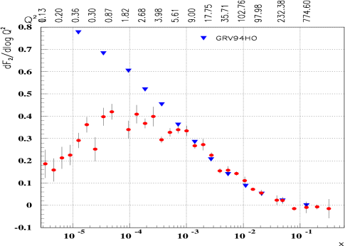
Figure 5: The Caldwell plot of HERA data.

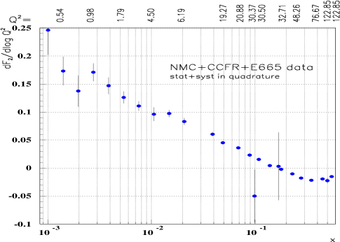
Figure 6: Caldwell’s compilation of points from fixed target experiments

with $P/q$ very large and $q/Q$ large but fixed independently of $1/x={2P\cdot q\over Q^{2}.}$ Thus all $x-evolution$ is included in the proton’s wavefunction and the scattering can be viewed as illustrated in Fig.4. Before the collision the virtual photon splits into a quark-antiquark pair which then interacts with the gluon field of the proton to produce an inelastic collision. A. Caldwell[34] suggested looking at $Q^{2}{\partial F_{2}(x,Q^{2})\over\partial Q^{2}}$ as a useful way of seeing very small-x effects at moderate $Q^{2}.$ This is useful because

$$Q^{2}{\partial F_{2}(x,Q^{2})\over\partial Q^{2}}\propto Q^{2}\sigma_{{q}\bar{q}}(\Delta x_{\perp}\sim 1/Q)$$ (32)

where $\sigma_{{q}\bar{q}}$ is the cross section of the ${q}\bar{q}$ pair to interact with the proton. The transverse coordinate separation of the pair is proportional to $1/Q.$ If gluons are reasonably dilute in the proton, so that the parton picture applies, one has

$$\sigma_{{q}\bar{q}}\propto{\alpha\over Q^{2}}\ xG(x,Q^{2})$$ (33)

with  $G$ the gluon distribution in the proton. The $1/Q^{2}$ on the right-hand side of (33) reflects the diluteness of gluons in the proton. On the other hand, if gluons are packed densely in the proton one reaches the unitarity limit and cross sections become geometric in which case

$$\sigma_{{q}\bar{q}}\ \propto\ \pi R_{0}^{2}$$ (34)

where $R_{0}$ is the radius of these proton. Using (33) and (34) in (32) we see that a signal for saturation is that $Q^{2}{\partial F_{2}\over\partial Q^{2}}$ should grow linearly in $Q^{2}.$ HERA data is shown in Fig.5 while fixed target data is shown in Fig.6. Data are plotted as a function of  $x$ on the lower axis and as a function of  $Q^{2}$ on the upper axis. The turnover in the HERA data at  $Q^{2}\approx 2,$ and the lack of such a turnover in the larger  $x$ fixed target data may be the indication of parton saturation for all transverse momenta less than about $1-1\ 1/2GeV$[35, 36, 37].

3.6 Why is equilibration nontrivial?

We have seen that there are a great many gluons in the wavefunction of a high energy heavy ion and that many of these gluons are likely freed in a central ion-ion collision. With the large gluon densities present it would seem to be a simple matter to reach equilibration. However, the gluons are located in a single layer, perpendicular to the axis of collision. Thus immediately after the collision the gluon density will begin to rapidly decrease and it is not certain, a priori, whether equilibration will set in before the system falls apart. There are some pretty good indications from Monte Carlo calculations[38, 39, 40] that kinetic equilibration does indeed occur at RHIC and LHC energies, however, it would be nice to see more clearly, in analytic calculation what the issues are and how certain it is that equilibration occurs. In what follows I give a very simplified version of a criterion for equilibration in the McLerran-Venugopalan model.

We imagine a head-on collision of two heavy ions each of which has gluons in its wavefunction saturated up to a scale  $Q.$  We suppose that during a time on the order of $1/Q$ the gluons having $k_{\perp}\leq Q,$ in the central unit of rapidity are freed while those having $k_{\perp}\geq Q$ are virtual fluctuations only and are not freed. Then follow a particular freed gluon in the central unit of rapidity. (We may suppose that $k_{\perp}$ of the gluon is $k_{\perp}\approx Q,$ since there is little phase space for $k_{\perp}<<Q$ and freed gluons having $k_{\perp}>>Q$ are few.) If this gluon has a collision with momentum transfer on the order of $Q$ it has gone a significant way toward equilibration. Thus as an equilibration criterion we take

$$1=\int_{\tau_{0}}^{\tau}{dt\over\lambda(t)},$$ (35)

where $\tau_{0}=1/Q,\lambda(t)$ is the mean free path and $\tau$ is some time which should obey $\tau\leq R.$ (If the gluon does not experience a hard scattering in $\tau\leq R$ it is unlikely that a later scattering will occur because the expansion becomes 3-dimensional rather than 1-dimensional.) Now

$${1\over\lambda(t)}=\rho_{g}(t)\sigma_{gg\to gg}$$ (36)

where

$$\rho_{g}\cdot\ g(t)={n_{g}^{max}\over t}={(N_{c}^{2}-1)Q^{2}\over 4\pi^{2}\alpha N_{c}t}$$ (37)

and

$$\sigma_{gg\to gg}=\bigl{(}{\alpha N_{c}\over\pi}\bigr{)}^{2}{4\pi^{3}\over(N_{c}^{2}-1)Q^{2}}$$ (38)

In using (37) we neglect the b-dependence of the saturation momentum. In (38) we have integrated ${d\sigma\over dt}=({\alpha N_{c}\over\pi})^{3}{4\pi^{3}\over(N_{c}^{2}-1)t^{2}}$ over $t$ from $-t=Q^{2}$ to $\infty.\ \alpha$ in (37) and (38) should be evaluated at $Q^{2}.$ Thus (35) becomes

$$1={\alpha N_{c}\over\pi}\ell n\ \tau/\tau_{0}$$ (39)

or, using $\alpha(Q^{2})={1\over b\ell nQ^{2}/\wedge^{2}}$ with $b={11N_{c}-2N_{f}\over 12\pi},$

$$\tau={1\over\wedge}({Q\over\wedge})^{2\pi\ b/N_{c}-1}.$$ (40)

Since $Q^{2}\propto R$ from (30) equilibration will occur if

$${\pi\ b\over N_{c}}-{1\over 2}\ <\ 1$$ (41)

which is the case. It is reassuring to see that the equilibration seems to be met in the McLereran-Venugopalan model, but it is , perhaps, a little disturbing that it seems to be accidental and not a fundamental property of high energy heavy ion collisions.

4 Perturbative versus nonperturbative QCD

Full nonperturbative calculations of physical quantities are desirable but hard to get in QCD. In hard probes of quark and gluon structure in hadrons the operator product expansion separates hard from soft physics where the hard part is calculable perturbatively and the soft part can be parametrized in a general way. The operator product expansion takes the form

$$\int e^{iqx}d^{4}x\ j(x)j(0)\mathrel{\longrightarrow\atop q^{2}large}{\cal{O}}_{1}E_{1}(\alpha(Q))+{1\over Q^{2}}{\cal{O}_{2}E_{2}(\alpha(Q))+\cdot\cdot\cdot}$$ (42)

where ${\cal{O}}_{1}$ is the leading twist term and ${\cal{O}}_{2}$ and the next- to-leading twist term with $E_{1}$ and $E_{2}$ coefficient functions. An interesting subtlety arises because $E_{1}$ has a divergent perturbation series

$$E_{1}(\alpha) = \sum_{n}E_{1n}\alpha^{n}$$ (43)

$$E_{1n}{\sim\atop n\ large} e_{1} n!\beta_{2}^{n}n^{\gamma}(1+0({1\over n})),$$

…

where $\beta_{2}$ is the first coefficient of the $\beta-$function. The ambiguity in the sum (40) due to the divergent perturbation series is of size $1/Q^{2}$ and means that the separation of the ${\cal{O}}_{1}$ and

$t{O}_{2}$ terms in (39) is not without ambiguity[41].

For example, for the $F_{3}$ structure function in neutrino proton scattering one commonly writes

$$xF_{3}(x,Q^{2})=xF_{3}^{LT}(x,Q^{2})+{h(x)\over Q^{2}}$$ (44)

with $F_{3}^{LT}$ the leading twist contribution and the $h/Q^{2}$ the higher twist term. Recently an interesting observation has been made by Kataev[9] and his collaborators that $h(x)$ depends on the level to which the perturbation theory analysis of $F_{3}^{LT}$ is done. If $F_{3}^{LT}$ is evaluated in a leading order renormalization group formalism a large $h(x)$ emerges from the fit. If a next-to-leading order formalism issued for $F_{3}^{LT}$ a somewhat smaller but still substantial contribution from $h$ is needed. When $F_{3}^{LT}$ is evaluated in a next-to-next-to-leading formalism very little room is left for $h.$ This is shown in Figs.7- 9 taken from Ref.9. I think there is an important lesson here. It is not clear how to separate leading and higher twist terms and the separation will depend on the level to which the perturbative calculation is done.

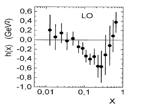
Figure 7: The results of the LO extraction of the x-shape of the twist-4 contribution h(x)

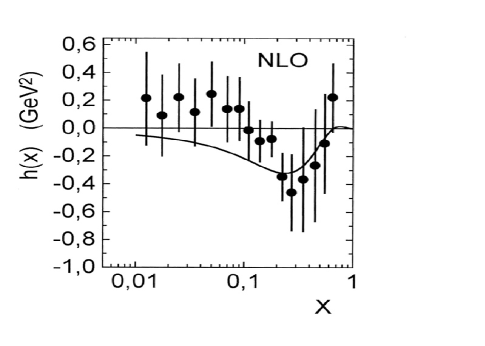
Figure 8: The results of the NLO extraction of the x-shape of the twist-4 contribution h(x). For comparison, the IRR-model prediction of Ref.[22], obtained using the NLO MRS parametrization, is also depicted.

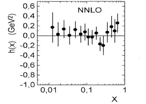
Figure 9: The results of the NNLO extraction of the x-shape of the twist-4 contribution $h(x).$

References

- [1] For a review see the lectures at the VIII Jorge André, Swieca Summer School (Brazil, February 1997) by G.P. Lepage, Nucl-th 9706029.
- [2] S. Weinberg, Phys.Lett.B251 (1990) 288; Nucl.Phys.B363 (1991)3.
- [3] C. Ordonez, U. van Kolck, Phys. Rev.Lett. 72 (1994) 1982.
- [4] T.S. Park, D.P. Min and M. Rho, Nucl.Phys.A596 (1996) 515.
- [5] D.B. Kaplan, M.J. Savage and M. B. Wise, Nucl. Phys. B478 (1996) 629.
- [6] D.B. Kaplan,M.-J. Savage and M. B. Wise, Nul.-th/9802075.
- [7] L. Cardman, talk given at this conference.
- [8] A. Magnon, talk given at this conference.
- [9] A.L. Katae, A.V. Kotikov, G. Parente and A.V. Sidorov, Phys.Lett.B417 (1998) 374.
- [10] For a review see “Hard Processes” by B.L. Ioffe, V.A. Khoze and L.N. Lipatov,North Holland (1984).
- [11] S.J. Brodsky and F. Schlumpf, Phys.Lett. B329 (1994) 111.
- [12] F.E. Close and R.G. Roberts, Phys.Lett. B316 (1993) 165.
- [13] C.S. Lam and B.-A. Li, Phys.Rev.D25 (1982) 683.
- [14] A.V. Efremov and O.V. Teryaev, Dubna Report E2-88-287.
- [15] G. Altarelli and G.G. Ross, Phys.Lett. B212 (1988) 391.
- [16] R.D. Carlitz, J.C. Collins and A.H. Mueller, Phys.Lett.B214 (1988) 229.
- [17] E154 Collaboration, K. Abe et al., Phys.Lett.B405 (1997) 180.
- [18] SMC Collaboration,B. Adeva et al., Phys.Lett.B412 (1997) 414.
- [19] G. Altarelli, R.D. Ball, S. Forte and G. Ridofi, hep-ph/9803237.
- [20] SAMPLE Collaboration, B. Mueller et al., Phys. Rev. Lett.78 (1997) 3824.
- [21] HAPPEX Collaboration, results presented at this conference by K.Kumar.
- [22] CCFR Collaboration, W.G. Seligman et al., Phys. Rev.Lett.79 (1997) 1213.
- [23] I thank Professor D. Beck for reminding me of this important result.
- [24] J.-P. Blaizot and A.H.Mueller, Nucl.Phys.B289 (1987) 847.
- [25] K. Kajantie, P.V. Landshoff and J. Lindfors, Phys. Rev.Lett.59 (1987) 2517.
- [26] K.J. Eskola, K. Kajantie and J. Lindfors, Nucl. Phys., B323 (1989)37.
- [27] J.K. Eskola, hep-ph/9708472.
- [28] K.J. Eskola, B. Mueller and X.-N. Wang, Phy.Lett.B374 (1996) 20.
- [29] L. McLerran and R. Venugopalan, Phys.Rev.D49 (1994) 2233; 49(1994) 3352; 50 (1994) 2225.
- [30] J. Jalilian-Marian, A. Kovner, L. McLerran and H. Weigert, Phys.Rev.D55 (1997) 5414.
- [31] Yu.V. Kovchegov, Phys.Rev.D54 (1996) 5463.
- [32] Yu.V. Kovchegov and A.H. Mueller, hep-ph/9805208.
- [33] L.V. Gribov, E.M. Levin and M.G. Ryskin, Phys. Rep.100 (1983) 1.
- [34] A. Caldwell, talk at DESY Workshop, September, 1997;See also H. Abramowicz and A. Caldwell,DESY report 98-192.
- [35] E. Gotsman, E. Levin and U. Maor, Phys.Lett.B425 (1998) 369.
- [36] A.H. Mueller, in DIS 98, Brussels.
- [37] K. Golec-Biernat and M. Wüsthoff, hep-ph/9807513.
- [38] K. Geiger, Com. Phys.Comm. 104 (1997) 70.
- [39] B. Zhang, Comp.Phys.Comm. 109 (1998) 193, and Thesis, Columbia University, 1998.
- [40] S. Wong, Phys.Rev.C54 (1996) 2588.
- [41] A.H. Mueller, Phys.Lett.B308 (1993) 355.