TAUP 2561 - 99

THE SURVIVAL PROBABILITY
OF LARGE RAPIDITY GAPS IN

A THREE CHANNEL MODEL

E. G O T S M A N¹⁾, E. L E V I N²⁾   and U.  M A O R³⁾

School of Physics and Astronomy
Raymond and Beverly Sackler Faculty of Exact Science
Tel Aviv University, Tel Aviv, 69978, ISRAEL

Abstract:

The values and energy dependence for the survival probability $<\mid S\mid^{2}>$ of large rapidity gaps (LRG) are calculated in a three channel model. This model includes single and double diffractive production, as well as elastic rescattering. It is shown that $<\mid S\mid^{2}>$ decreases with increasing energy, in line with recent results for LRG dijet production at the Tevatron. This is in spite of the weak dependence on energy of the ratio $(\sigma_{el}+\sigma_{SD})/\sigma_{tot}$.

1 Introduction

A large rapidity gap ( LRG ) process is defined as one where no hadrons are produced in a sufficiently large rapidity region. Historically, both Dokshitzer et al.[1] and Bjorken[2], suggested utilizing LRG as a signature for Higgs production in a W-W fusion process, in hadron-hadron collisions. It turns out that the LRG processes give a unique opportunity to measure the high energy asymptotic behaviour of the amplitudes at short distances, where one can use the developed methods of perturbative QCD ( pQCD ) to calculate the amplitudes. Consider a typical LRG process - the production of two jets with large transverse momenta $\vec{p}_{t1}\,\,\approx\,\,-\vec{p}_{t2}\,\,\gg\,\,\mu$, with a LRG between the two jets. $\mu$ is a typical mass scale of “soft” interactions. We have the reaction

$$p(1)\,\,+\,\,p(2)\,\,\longrightarrow\,\,M_{1}[hadrons\,\,+\,\,jet_{1}(y_{1},p_{t1})]$$ (1)

$$+\,\,LRG[\Delta y=|y_{1}-y_{2}|]\,\,+\,\,M_{2}[hadrons\,\,+\,\,jet_{2}(y_{2},p_{t2})]$$

where $y_{1}$ and $y_{2}$ are the rapidities of the jets and $\Delta y=|y_{1}-y_{2}|\,\,\gg\,\,1$. The production of two jets with LRG between them can occur because:

1. A fluctuation in the rapidity distribution of a typical inelastic event. However, the probability for such a fluctuation is proportional to $e^{-\frac{\Delta y}{L}}$, where $L$ denotes the value of the correlation length. We can evaluate $L\,\approx\,\frac{1}{\frac{dn}{dy}}$, where $\frac{dn}{dy}$ is the number of particles per unit in rapidity. A LRG means that $\Delta y\,\gg\,L$ and so the probability is small;

2. The exchange of a colourless state in QCD. This exchange is given by the amplitude of the high energy interaction at short distances. We denote it as a “hard” Pomeron in Fig.1. We denote by $F_{s}$ the ratio of the cross section due to this Pomeron exchange, to the typical inelastic event cross section generated by gluon exchange ( see Fig. 1 ). In QCD we do not expect this ratio to decrease as a function of the rapidity gap $\Delta y=y_{1}-y_{2}$. For a BFKL Pomeron[3], we expect an increase once $\Delta y\,\gg\,\,1$. Using a simple QCD model for the Pomeron , namely, that it can be approximated by two gluon exchange[4], Bjorken[2] gave the first estimate for $F_{s}\,\approx\,\,0.15$, which is unexpectantly large.

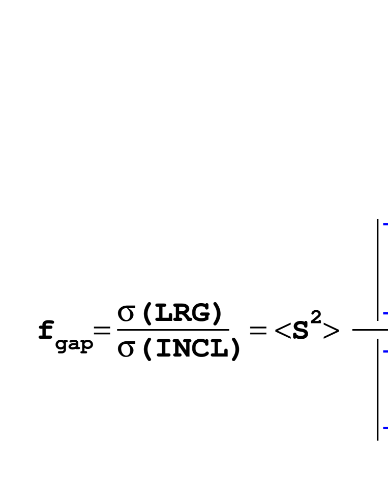
Figure 1: Pictorial definition of $f_{gap}$, where P and G represent respectively, the exchange of a colour singlet and a colour octet.

As noted by Bjorken, we are not able to measure $F_{s}$ directly in a LRG experiment. The experimentally measured ratio of the number of events with a LRG, to the number of events without a LRG ( see Fig. 1 ) is not equal to $F_{s}$, but has to be modified by an extra factor which we call the survival probability of LRG.

$$f_{gap}=<\mid S\mid^{2}>\,\times\,F_{s}\,\,.$$ (2)

The appearance of $<\mid S\mid^{2}>$ in Eq. (2) has a very simple physical interpretation. It is the probability that the rapidity gap due to Pomeron exchange, will not be filled by the produced particles ( partons and/or hadrons ) from the rescattering of spectator partons ( see Fig.2a ), or from the emission of bremsstrahlung gluons from partons taking part in the “hard” interaction, or from the “hard” Pomeron ( see Fig. 2b ).

$$<\mid S\mid^{2}>\,\,\,=\,\,\,<\mid S_{bremsstrahlung}(\,\Delta y\,\,=\,\,|\,y_{1}\,\,-\,\,y_{2}\,|\,)\mid^{2}>\,\,\times\,\,<\mid S_{spectator}(\,s\,)\mid^{2}>\,\,,$$ (3)

where $s$ denotes the total c.m. energy squared.

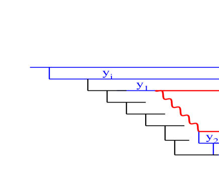
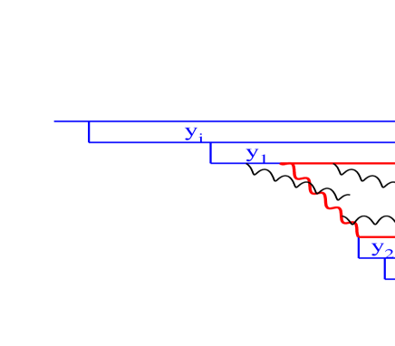
Fig. 2-a	Fig. 2-b

Figure 2: Rescatterings of the spectator partons ( Fig.2a ) and emission of the bremsstrahlung gluons ( Fig.2b ) that fill the LRG .

• $<\mid S_{bremsstrahlung}(\,\Delta y\,)\mid^{2}>$ can be calculated in pQCD[5], it depends on the kinematics of each specific process, and on the value of the LRG .

• To calculate $<\mid S_{spectator}(\,s\,)\mid^{2}>$ we need to find the probability that all partons with rapidity $y_{i}\,>\,y_{1}$ in the first hadron ( see Fig.2a ) and all partons with $y_{j}\,<\,y_{2}$ in the second hadron do not interact inelastically and, hence, do not produce additional hadrons in the LRG. This is a difficult problem, since not only partons at short distances contribute to such a calculation, but also partons at long distances for which the pQCD approach is not valid. Many attempts have been made to estimate $<\mid S_{spectator}(\,s\,)\mid^{2}>$[2][6][7][8][9][10][11], but this problem still awaits a solution.

On the other hand, the experimental studies of LRG processes have progressed, and have yielded interesting results both at the Tevatron[12][13], and at HERA[14].

The main results of the experimental data pertaining to the survival probability are:

• the value of $<\mid S\mid^{2}>$ is rather small. Indeed, the experimental values for $f_{gap}(\,\sqrt{s}\,=\,630\,GeV\,)\,=\,1.6\,\pm 0.2\%$ ( D0[13]) $=\,2.7\,\pm 0.9\%$ ( CDF[12] ) and $f_{gap}(\,\sqrt{s}\,=\,1800\,GeV\,)\,=\,0.6\,\pm\,0.2\%$ ( D0[13] ) $=1.13\,\pm\,0.16\%$ ( CDF[12] ) can be understood only if $<\mid S\mid^{2}>\,\,\approx\,\,1-10\%$;

• the energy dependence of $f_{gap}$, namely, the obsevation that[12][13]

  $$R^{CDF}_{gap}\,\,=\,\,\frac{f_{gap}(\sqrt{s}=630\;GeV)}{f_{gap}(\sqrt{s}\;=\;1800\;GeV)}\;\;=\;\;2.4\;\;\pm\,\,0.9$$

  $$R^{D0}_{gap}\,\,=\,\,\frac{f_{gap}(\sqrt{s}=630\;GeV)}{f_{gap}(\sqrt{s}\;=\;1800\;GeV)}\;\;=\;\;2.67\;\;\pm\,\,0.38$$

  leads to $<\mid S\mid^{2}>$ which decreases by a factor two in the above range of energy. So, we expect that

  $$R_{S}\,\,=\,\,\frac{<\mid S\mid^{2}>_{\sqrt{s}=630}}{<\mid S\mid^{2}>_{\sqrt{s}=1800}}\;\;\approx\;\;2\,\,.$$

  A recent D0 estimate[13] of the above ratio is $2.2\,\pm\,0.8$.

It was shown in Ref.[11] that the Eikonal Model for the “soft” interaction at high energies, is able to describe the features of the experimental data. However, we may question the reliability of this approach. Especially worrying, is the energy dependence of $<\mid S\mid^{2}>$, since a natural parameter related to the parton rescatterings is the ratio

$$R_{D}\,\,\,=\,\,\,\frac{\sigma_{D}}{\sigma_{tot}}\,\,\,\equiv\,\,\,\frac{\sigma_{el}\,\,+\,\,\sigma_{SD}\,\,+\,\,\,\sigma_{DD}}{\sigma_{tot}}\,\,,$$ (4)

where $\sigma_{SD}$ and $\sigma_{DD}$ are the cross sections of single and double diffraction. Experimentally, $R_{D}$ is approximately constant over a wide range of energy. In the Eikonal Model we consider $\sigma_{SD}\,\,\ll\,\,\sigma_{el}$ and $\sigma_{DD}\,\,\ll\,\,\sigma_{el}$ and, therefore, we model $R_{D}\,\,\rightarrow\,\,R_{el}\,\,=\,\,\frac{\sigma_{el}}{\sigma_{tot}}$. Experimentally, $R_{el}$ depends on energy, which gives rise to a considerable decrease of the survival probability. Indeed, the first attempt to take into account the parameter $R_{D}$ in the calculation of $<\mid S\mid^{2}>$ given in Ref.[9], leads to

$$<\mid S\mid^{2}>\,\,=\,\,[\,1\,\,-\,\,2\,\,R_{D}\,]^{2}\,\,,$$ (5)

which yields a reasonable value of the survival probability, but cannot account for its substantial dependence on energy ( see Ref.[11] ).

The main goal of this paper is to develop a simple model for the “soft” high energy interactions, which correctly includes the processes of diffractive dissociation, and to study the value and energy dependence of $<\mid S_{spectator}(\,s\,)\mid^{2}>$. In the next section we develop our approach, while in section 3 we discuss the value of $<\mid S_{spectator}(\,s\,)\mid^{2}>$ in a model which describes the energy dependence of $R_{el}$ and $R_{D}$. We show that our model gives the experimentally observed decrease of the survival probability as a function of energy. In section 4 we discuss and summarize our results.

2 A three channel model

2.1 Diffractive dissociation ( general approach )

Diffractive dissociation is the simplest process with a LRG in which no hadrons are produced in the central rapidity region. In these processes we have production of one ( single diffraction (SD) ) or two groups of hadrons ( double diffraction ( DD ) ) with masses ( $M_{1}$ and $M_{2}$ in Fig.3 ) much less than the total energy ( $M_{1}\,\ll\,\sqrt{s}$ and $M_{2}\,\ll\,\sqrt{s}$ ).

Figure 3: Lego - plot for double diffractive dissociation.

From a theoretical point of view, as was suggested by Feinberg[15] and Good and Walker[16], diffractive dissociation can be viewed as a typical quantum mechanical process which occurs since the hadron states are not diagonal with respect to the strong interaction scattering matrix.

We consider this point in more detail, and denote the wave functions which are diagonal with respect to the strong interaction by $\Psi_{n}$. The quantum numbers $n$ are called the correct degrees of freedom at high energy. The amplitude of the high energy interaction is, therefore, given by

$$A_{n_{1}n_{2}}\,\,=\,\,<\Psi_{n_{1}}\Psi_{n_{2}}|T|\Psi_{n_{1}^{\prime}}\Psi_{n_{2}^{\prime}}>\,\,=\,\,A_{n_{1},n_{2}}\,\delta_{n_{1},n_{1}^{\prime}}\,\delta_{n_{2},n_{2}^{\prime}}\,\,,$$ (6)

where the brackets denote all needed integrations and $T$ is the scattering matrix.

The wave function of a hadron is

$$\Psi_{hadron}\,\,\,=\,\,\,\sum^{\infty}_{n=1}\,C_{n}\,\Psi_{n}\,\,.$$ (7)

For a hadron - hadron interaction we have a wave function $\Psi_{hadron}\,\times\,\Psi_{hadron}$ before the collision, while after the collision the scattering matrix $T$ gives a new wave function

$$\Psi_{final}\,\,\,=$$

$$\sum^{\infty}_{n_{1}=1}\,\sum^{\infty}_{n_{2}=1}\,\sum^{\infty}_{n_{1}^{\prime}=1}\,\sum^{\infty}_{n_{2}^{\prime}=1}\,\,C_{n_{1}}\,C_{n_{2}}<\Psi_{n_{1}}\,\Psi_{n_{2}}|T|\Psi_{n_{1}^{\prime}}\,\Psi_{n_{2}^{\prime}}>\Psi_{n_{1}^{\prime}}\,\Psi_{n_{2}^{\prime}}\,\,=$$

$$\,\,\sum^{\infty}_{n_{1}=1}\,\sum^{\infty}_{n_{2}=1}\,\,C_{n_{1}}\,C_{n_{2}}\,A_{n_{1},n_{2}}\,\Psi_{n_{1}}\,\Psi_{n_{2}}\,\,.$$ (8)

Eq. (2.1) leads to the elastic amplitude

$$a_{el}\,\,=\,\,<\Psi_{final}|\Psi_{hadron}\,\times\,\Psi_{hadron}>\,\,=\,\,\sum^{\infty}_{n_{1}=1}\,\,\sum^{\infty}_{n_{2}=1}\,\,C^{2}_{n_{1}}\,\,C^{2}_{n_{2}}\,\,\,A_{n_{1},n_{2}}\,\,,$$ (9)

and to another process, namely, to the production of other hadron states, since $\Psi_{final}$ may be different from $\Psi_{hadron}\,\times\,\Psi_{hadron}$.

$$\sigma_{D}(s,b)\,\,=\,\,<\Psi_{final}|\Psi_{final}>\,\,-\,\,<\Psi_{final}|\Psi_{hadron}\,\times\,\Psi_{hadron}>^{2}\,\,=$$

$$\sum^{\infty}_{n_{1}=1}\,\sum^{\infty}_{n_{2}=1}\,\,C^{2}_{n_{1}}\,C^{2}_{n_{1}}\,A^{2}_{n_{1},n_{2}}\,\,-\,\,\left(\,\sum^{\infty}_{n_{1}=1}\,\,\sum^{\infty}_{n_{2}=1}\,\,C^{2}_{n_{1}}\,\,C^{2}_{n_{2}}\,\,\,A_{n_{1},n_{2}}\,\,\right)^{2}\,\,.$$ (10)

Using the normalization condition for the hadron wave function ( $\sum_{n}\,C^{2}_{n}\,\,=\,\,1$ ), the cross section of the diffractive dissociation processes, Eq. (2.1), can be reduced to the form[16][17]

$$\sigma_{D}(s,b)\,\,=\,\,<|\sigma^{2}(s,b)|>\,\,-\,\,<|\sigma(s,b)|>^{2}\,\,,$$ (11)

where $<|f|>\,\,\equiv\,\,\sum_{n_{1}}\,\,\sum_{n_{2}}\,\,C^{2}_{n_{1}}\,C^{2}_{n_{2}}\,\,f_{n_{1},n_{2}}$ and we have returned to our original variables: energy ( $s$ ) and impact parameter ( $b$ ).

2.2 Diffractive dissociation and shadowing corrections

For $A_{n_{1},n_{2}}(s,b)$, and only for $A_{n_{1},n_{2}}(s,b)$, we have the unitarity constraint

$$2\,\,ImA^{el}_{n_{1},n_{2}}(s,b)\,\,=\,\,|A^{el}_{n_{1},n_{2}}(s,b)|^{2}\,\,+\,\,G^{in}_{n_{1},n_{2}}(s,b)\,\,.$$ (12)

Assuming that the amplitude at high energy is predominantly imaginary, we obtain the solution of Eq. (12)

$$A^{el}_{n_{1},n_{2}}(s,b)\,\,\,=\,\,\,i\,\left(\,1\,\,\,-\,\,\,e^{-\,\frac{\Omega_{n_{1},n_{2}}(s,b)}{2}}\,\right)\,\,;$$ (13)

$$G^{in}_{n_{1},n_{2}}(s,b)\,\,\,=\,\,\,1\,\,\,-\,\,\,e^{-\,\Omega_{n_{1},n_{2}}(s,b)}\,\,.$$ (14)

To find a relation between the processes of diffraction dissociation and the value of the shadowing corrections ( SC ), we assume that $\Omega_{n_{1},n_{2}}(s,b)\,\,\ll\,\,1$ and expand Eq. (12) - Eq. (14) with respect to $\Omega_{n_{1},n_{2}}$

$$A^{el}_{n_{1},n_{2}}(s,b)\,\,=\,\,\frac{\Omega_{n_{1},n_{2}}(s,b)}{2}\,\,\,-\,\,\frac{\Omega^{2}_{n_{1},n_{2}}(s,b)}{8}\,\,\,+\,\,\,O(\Omega^{3}_{n_{1},n_{2}})\,\,;$$ (15)

$$G^{in}_{n_{1},n_{2}}(s,b)\,\,\,=\,\,\,\Omega_{n_{1},n_{2}}(s,b)\,\,\,-\,\,\,\frac{\Omega^{2}_{n_{1},n_{2}}(s,b)}{2}\,\,\,+\,\,\,O(\Omega^{3}_{n_{1},n_{2}})\,\,.$$ (16)

Using Eq. (7) - Eq. (2.1) we obtain for the observables

$$\sigma_{el}(s,b)\,\,\,=\,\,\,\frac{1}{4}\,\,\left(\,\sum^{\infty}_{n_{1}=1}\,\sum^{\infty}_{n_{2}=1}\,C^{2}_{n_{1}}\,C^{2}_{n_{2}}\,\Omega_{n_{1},n_{2}}(s,b)\,\right)^{2}$$ (17)

$$\sigma_{tot}\,=\,\sum^{\infty}_{n_{1}=1}\,\sum^{\infty}_{n_{2}=1}\,\,C^{2}_{n_{1}}\,C^{2}_{n_{2}}\,\Omega_{n_{1},n_{2}}(s,b)\,-\,\frac{1}{4}\,\left(\,\sum^{\infty}_{n_{1}=1}\,\sum^{\infty}_{n_{2}=1}\,\,\,C^{2}_{n_{1}}\,C^{2}_{n_{2}}\,\Omega^{2}_{n_{1},n_{2}}(s,b)\,\right)$$ (18)

$$\sigma_{in}\,=\,\sum^{\infty}_{n_{1}=1}\,\sum^{\infty}_{n_{2}=1}\,\,\,C^{2}_{n_{1}}\,C^{2}_{n_{2}}\Omega_{n_{1},n_{2}}(s,b)\,-\,\frac{1}{2}\,\left(\,\sum^{\infty}_{n_{1}=1}\,\sum^{\infty}_{n_{2}=1}\,\,\,C^{2}_{n_{1}}\,C^{2}_{n_{2}}\Omega^{2}_{n_{1},n_{2}}(s,b)\,\right)$$ (19)

$$\sigma_{diff}\,=\,\frac{1}{4}\,\{\sum^{\infty}_{n_{1}=1}\,\sum^{\infty}_{n_{2}=1}\,C^{2}_{n_{1}}\,C^{2}_{n_{2}}\,\Omega^{2}_{n_{1},n_{2}}(s,b)-\left(\,\sum^{\infty}_{n_{1}=1}\,\sum^{\infty}_{n_{2}=1}\,C^{2}_{n_{1}}\,C^{2}_{n_{2}}\Omega_{n_{1},n_{2}}(s,b)\,\right)^{2}\}.$$ (20)

In the parton model, one Pomeron exchange corresponds to a typical inelastic event with a production of a large number of particles. In this case, we can associate this exchange with $\Omega$, consequently $\sigma^{P}_{tot}(s,b)\,\,=\,\,\sigma^{P}_{in}(s,b)\,\,\propto\,\,\Omega$. All terms which are proportional to $\Omega^{2}$ describe two Pomeron exchange, and they induce SC.

We can evaluate the scale of the SC using experimental data on $\sigma_{tot},\sigma_{el}$ and $\sigma_{SD}$. Indeed, we can write the expression for the total cross section in the form

$$\sigma_{tot}\,\,\,=\,\,\sigma^{P}_{tot}\,\,\,-\,\,\,\Delta\sigma^{SC}_{tot}\,\,,$$ (21)

where $\sigma^{P}_{tot}$ is the contribution of Pomeron exchange to the total cross section. Summing Eq. (17) and Eq. (20) we derive that

$$\Delta\sigma^{SC}_{tot}\,\,=\,\,\sigma_{el}\,\,+\,\,\sigma_{diff}\,\,=\,\,\sigma_{el}\,\,+\,\,\sigma_{SD}\,\,+\,\,\sigma_{DD}\,\,=\,\,\sigma_{D}\,\,.$$ (22)

The ratio $R_{D}$ ( see Eq. (5) ) gives the scale of the SC in the situation when these are sufficiently weak ( $\Omega_{n_{1},n_{2}}\,\,\ll\,\,1$ ), since Eq. (22) can be rewritten in the form

$$R_{D}\,\,=\,\,\frac{\Delta\,\sigma^{SC}_{tot}}{\sigma_{tot}}\,\,.$$ (23)

Fig.4b shows that over a wide range of energy $R_{D}\,\,\approx\,\,0.34$ , and it appears to be independent of energy. The large value of $R_{D}$ implies that SC should be taken into account, and that SC lead to the small value of the survival probability. The almost constant $R_{D}$ suggests that the SC cannot induce the observed strong energy dependence of the survival probability. However, the value of $R_{D}$ is so large that we have to develop an approach to calculate SC for $\Omega_{n_{1},n_{2}}\,\,\approx\,\,1$.

Fig. 4-a	Fig.4-b

Figure 4: The experimental data on the ratio $R_{el}\,=\,\sigma_{el}/\sigma_{tot}$ ( Fig.4a ) and on the ratio $R_{D}\,=\,(\sigma_{el}+\sigma_{SD}+\sigma_{DD})/\sigma_{tot}$ ( Fig.4b ) versus $\log(s/s_{0})$ with $s_{0}=1\,GeV^{2}$.

2.3 The Eikonal Model

We first discuss the Eikonal model. This is an approximation which has been widely used to estimate the value of the SC, in a situation when they are not small. The main assumption of this model is that hadrons are the correct degrees of freedom at high energy. In other words, we assume that the interaction matrix is diagonal with respect to hadrons. From Eq. (7) - Eq. (11) one can see that this model does not include diffractive dissociation processes. Therefore, the accuracy of our estimates in the Eikonal Model will be given by the ratio $(\sigma_{SD}+\sigma_{DD})/\sigma_{el}$. From Fig.4 one can see that this ratio is about 1 at $\sqrt{s}\,\,\approx\,\,20\,GeV$ and decreases reaching the value of about 0.4 - 0.5 at the Tevatron energies. Thus, we cannot expect the Eikonal approach to yield a reasonable estimate. However, this model has the advantage of being simple, and it provides a good illustration, given below, of the main elements and approximations used in previous calculations.

1. Assumptions:

   • Hadrons are the correct degrees of freedom at high energies ;

   • $\sigma_{SD}\,\,\ll\,\,\sigma_{el}$ and $\sigma_{DD}\,\,\ll\,\,\sigma_{el}$ ;

   • At high energy the scattering amplitude is almost pure imaginary $Re\,a_{el}\,\,\ll\,\,Im\,a_{el}$ ;

   • Only the fastest partons can interact with each other  .

   The last assumption is the most restrictive, and clearly indicates how far from reality the Eikonal Model estimates could be.

2. Unitarity:

   In the Eikonal Model we only have one amplitude, since the scattering matrix is diagonal in the hadronic wave functions. Therefore, the unitarity constraints of Eq. (12) simplify to

   $$2\,\,Im\,a_{el}(s,b)\,\,=\,\,|a_{el}(s,b)|^{2}\,\,+\,\,G^{in}(s,b)\,\,.$$ (24)

   Eq. (24) has the solution

   $$a_{el}(s,b)\,\,\,=\,\,\,i\,\left(\,1\,\,\,-\,\,\,e^{-\,\frac{\Omega(s,b)}{2}}\,\right)\,\,;$$ (25)

   $$G^{in}(s,b)\,\,\,=\,\,\,1\,\,\,-\,\,\,e^{-\,\Omega(s,b)}\,\,.$$ (26)

3. The Pomeron hypothesis:

   The main assumption of the Eikonal Model is the identification of the opacity $\Omega(s,b)$ with a single Pomeron exchange, namely

   $$\Omega(s,b)\,=\,\Omega^{P}(s,b)\,\,;$$ (27)

   $$\Omega^{P}(s,b)\,\,=\,\,\sigma_{0}\,\Gamma(b)\,\,=\,\,\frac{\sigma_{0}}{\pi R^{2}(s)}\,(\frac{s}{s_{0}})^{\Delta_{P}}\,e^{-\frac{b^{2}}{R^{2}(s)}}\,\,=\,\,\nu(s)\,\,e^{-\frac{b^{2}}{R^{2}(s)}}\,;$$ (28)

   $$R^{2}(s)\,=\,\,4\,R^{2}_{0}\,\,+\,\,4\alpha^{\prime}_{P}\,\ln(s/s_{0})\,\,;$$ (29)

   $$\nu(s)\,\,=\,\,\frac{\sigma_{0}}{\pi R^{2}(s)}\,(\frac{s}{s_{0}})^{\Delta_{P}}\,\,=\,\,\Omega^{P}(s,b=0)\,\,.$$ (30)

   We assume a Pomeron trajectory $\alpha_{P}(t)\,=\,\alpha_{P}(0)\,\,+\,\,\alpha_{P}^{\prime}\,t$. Eq. (27) is a reasonable approximation in the kinematic region where $\Omega$ is small, i.e. either at low energies or at high energies when $b$ is large. Therefore, the Eikonal approach is the natural generalization of the single Pomeron exchange satisfying $s$-channel unitarity. Eq. (27) is an explicit analytic expression for the well known partonic picture for the Pomeron structure, namely, the single Pomeron exchange is responsible for the inelastic production of particles which are uniformly distributed in rapidity.

4. Exponential parameterization:

   In Eq. (28) a Gaussian form is explicitly assumed for the profile function $\Gamma(b)$. This corresponds to an exponential form in $t$ space.

   $$\Gamma(b)\,\,\,=\,\,\frac{1}{\pi\,R^{2}(s)}\,\,e^{-\frac{b^{2}}{R^{2}(s)}}\,\,.$$ (31)

   This form is assumed due to its simplicity, the resulting integrals can be done analytically and we can write the explicit answer for the physical observables. The proper definition of the profile function $\Gamma(b)$ is given by the following Fourier transform

   $$\Gamma(b)\,\,\,=\,\,\frac{1}{2\pi}\int\,\,d^{2}b\,\,e^{-i\mathbf{\vec{q}\,\cdot\vec{b}}}\,\,G^{2}_{P}(q^{2})\,\,,$$ (32)

   where $G_{P}(q^{2})$ is the Pomeron form factor. For example, one can take for $G_{P}(q^{2})$ the prediction of the Additive Quark Model ( see Ref.[18] ) in which $G_{P}(q^{2})\,\,=\,\,G_{em}$, where $G_{em}$ is the electromagnetic form factor of a hadron.

5. $\mathbf{R_{D}}$ :

   Using Eq. (27) - Eq. (30) one can obtain a closed expression for the “soft” observables

   $$\sigma_{tot}\,\,=\,\,2\,\pi\,R^{2}(s)\,\{\,\ln(\nu(s)/2)\,\,+\,\,C\,\,-\,Ei(-\nu/2)\,\}\,\,;$$ (33)

   $$\sigma_{in}\,\,=\,\,\,\pi\,R^{2}(s)\,\{\,\ln(\nu(s))\,\,+\,\,C\,\,-\,Ei(-\nu)\,\}\,\,;$$ (34)

   $$\sigma_{el}(s)\,\,=\,\,\sigma_{tot}(s)\,\,-\,\,\sigma_{in}(s)\,\,;$$ (35)

   where $Ei(x)\,\,\,=\,\,\int^{x}_{-\infty}\,\,\frac{e^{t}}{t}\,dt$ and $C\,\,=\,\,0.5773$.

   We define

   $$R_{el}\,\,=\,\,\frac{\sigma_{el}}{\sigma_{tot}}\,\,=\,\,\frac{\ln[\frac{\nu}{4}]\,\,+\,\,C\,\,+\,\,Ei(-\nu)\,\,-\,\,2\,Ei(-\frac{\nu}{2})}{2\,[\,\ln[\frac{\nu}{2}]\,\,+\,\,C\,\,-\,\,Ei(-\frac{\nu}{2})\,]}\,\,.$$ (36)

   Note, that the ratio $R_{el}$ depends only on $\nu$ and does not depend on the value of radius. Using Eq. (36) one can find the value of $\nu$ from the experimental data on $R_{el}$ ( see Fig.4a ) this was done in Ref.[11]. With the value of $\nu$ determined in this way we can calculate the survival probability.

6. Survival probability :

   From Eq. (26) one can conclude that the factor

   $$P(s,b)\,\,\,=\,\,\,e^{-\Omega(s,b)}\,\,,$$ (37)

   is the probability that the two initial hadrons do not interact inelastically. In a QCD approach, this means that the fastest parton from one hadron does not interact with the fastest parton from another. Therefore, in the Eikonal Model the survival probability can be easily calculated in the following way[2][6]

   $$<\mid S_{spectator}(\,s\,)\mid^{2}>\,\,\,=\,\,\,\frac{\int\,\,d^{2}b\,P(s,b)\,A_{HP}(\Delta y,b)}{\int\,\,d^{2}bA_{HP}(\Delta y,b)}\,\,,$$ (38)

   where $A_{HP}(\Delta y,b)$ is the cross section for a two parton jet production with a LRG due to single “hard” Pomeron exchange ( see Fig. 1 ). It has been proven that for a “hard” cross section, the $b$ dependence can be factorized out[7][19][20]. If we assume $A_{HP}(\Delta y,b)$ to be Gaussian we have

   $$A_{HP}(\Delta y,b)\,\,\,=\,\,\,\sigma_{HP}(\Delta y)\,\Gamma_{H}(b)\,\,\,=\,\,\frac{\sigma_{HP}(\Delta y)}{\pi R^{2}_{H}}\,\,e^{-\frac{b^{2}}{R^{2}_{H}}}\,\,,$$ (39)

   where $R^{2}_{H}$ is the radius of the “hard” interaction.

   Based on this assumption we obtain for the survival probability:

   $$<\mid S_{spectator}(\,s\,)\mid^{2}>=\frac{a\gamma[a,\nu]}{\nu^{a}}\,\,,$$ (40)

   where the incomplete gamma function $\gamma(a,x)=\int_{0}^{x}z^{a-1}e^{-z}dz$ and $a\,\,=\,\,\frac{R^{2}(s)}{R^{2}_{H}}\,\,.$

In Ref.[11], Eq. (36) and Eq. (40) were used to calculate the value and energy dependence of the survival probability. It was shown that both the value and the energy dependence are sensitive to the value of the “hard” radius, which was extracted in Ref.[11] from the experimental data on (i) vector meson diffractive dissociation in DIS at HERA[25], and on (ii) the CDF double parton cross section at the Tevatron[21].

Even though the Eikonal Model, as used in Ref.[11], can reproduce both the experimentally measured value and its energy behaviour, the reliability of such an approach is questionable. In the following we attempt to construct a more realistic model.

2.4 A three channel model: assumptions and general formulae

We want to construct a model which takes into account the processes of diffractive dissociation, for the case when these are not small ( $\sigma_{SD}\,\,\approx\,\,\sigma_{el}$ ).

2.4.1 Assumptions:

The main idea behind the model which is presented here, is to replace the many final states of the diffractively produced hadrons by one state ( effective hadron ). Doing so, we assume that we have two wave functions which are diagonal with respect to the strong interactions: $\Psi_{1}$ and $\Psi_{2}$. In this case the general Eq. (7) can be reduced to the form

$$\Psi_{hadron}\,\,\,=\,\,\,\alpha\,\Psi_{1}\,\,\,+\,\,\,\beta\,\Psi_{2}\,\,\,,$$ (41)

with the condition $\alpha^{2}\,+\,\beta^{2}\,\,=\,\,1$, which follows from the normalization of the wave function. The wave function of the diffractively produced bunch of hadrons should be orthogonal to $\Psi_{hadron}$ and has the form

$$\Psi_{D}\,\,\,=\,\,\,-\,\beta\,\Psi_{1}\,\,\,+\,\,\,\alpha\,\Psi_{2}\,\,.$$ (42)

Eq. (42) is the explicit form of our assumption, that we replace the complicated final state of diffractively produced systems of hadrons by one wave function $\Psi_{D}$.

2.4.2 General formulae:

Substituting Eq. (41) and Eq. (42) in Eq. (2.1) we can obtain

$$\Psi_{final}\,\,\,=\,\,\alpha^{2}\,A_{1,1}\Psi_{1}\,\times\,\Psi_{1}\,\,+\,\,\alpha\,\beta\,A_{1,2}\,[\,\Psi_{1}\,\times\,\Psi_{2}\,\,+\,\,\Psi_{2}\,\times\,\Psi_{1}\,]\,\,+\,\,\beta^{2}\,A_{2,2}\,\Psi_{2}\,\times\,\Psi_{2}\,\,.$$ (43)

The amplitudes $A_{i,k}\,\,(i,k=1,2)$ can be written in the form of Eq. (13) and Eq. (14) ( see Fig.5 )

$$A^{el}_{i,k}(s,b)\,\,=\,\,i\,\{\,\,1\,\,\,-\,\,\,e^{-\frac{\Omega_{i,k}(s,b)}{2}}\,\,\}\,\,;$$ (44)

$$G^{in}_{i,k}(s,b)\,\,\,=\,\,\,1\,\,\,-\,\,\,e^{-\Omega_{i,k}(s,b)}\,\,.$$ (45)

The elastic amplitude is equal to

$$a_{el}(s,b)\,\,=\,\,<\,\Psi_{hadron}\,\times\,\Psi_{hadron}\,|T|\,\Psi_{hadron}\,\times\,\Psi_{hadron}\,>\,\,=\,\,<\,\Psi_{hadron}\,\times\,\Psi_{hadron}|\Psi_{final}\,>\,\,=$$

$$\alpha^{4}\,A_{1,1}\,\,+\,\,2\,\alpha^{2}\,\beta^{2}\,A_{1,2}\,\,+\,\,\beta^{4}\,\,A_{2,2}\,\,.$$ (46)

For single diffraction we have the amplitude

$$a_{SD}(s,b)\,\,=\,\,<\,\Psi_{hadron}\,\times\,\Psi_{hadron}\,|T|\,\Psi_{D}\,\times\,\Psi_{hadron}\,>\,\,=\,\,<\,\Psi_{hadron}\,\times\,\Psi_{D}|\Psi_{final}\,>\,\,=$$

$$\alpha\,\beta\,\{\,\,-\,\alpha^{2}\,A_{1,1}\,\,+\,\,(\,\alpha^{2}\,-\,\beta^{2}\,)\,A_{1,2}\,\,+\,\,\beta^{2}\,\,A_{2,2}\,\,\}\,\,,$$ (47)

while the amplitude for double diffractive production is

$$a_{DD}(s,b)\,\,=\,\,<\,\Psi_{hadron}\,\times\,\Psi_{hadron}\,|T|\,\Psi_{D}\,\times\,\Psi_{D}\,>\,\,=\,\,<\,\Psi_{D}\,\times\,\Psi_{D}|\Psi_{final}\,>\,\,=$$ (48)

$$\alpha^{2}\,\beta^{2}\,\{\,\,A_{1,1}\,\,-\,\,2\,A_{1,2}\,\,+\,\,A_{2,2}\,\,\}\,\,.$$

Eq. (46) - Eq. (48) together with Eq. (44) and Eq. (45) give the general formulae for our model.

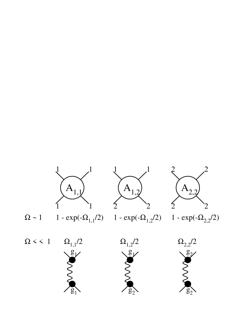
Figure 5: Solution of the unitarity constraints and the Regge parametrization for the correct degrees of freedom in the three channel model. The waved lines denote the exchange of the Pomeron.

In general this, three channel model is an attempt to sum all rescatterings shown in Fig.6. All of them are eikonal type rescatterings, but contrary to the Eikonal Model, the quasi-elastic rescatterings with production and rescattering of an effective diffractive state has been taken into account.

Figure 6: The Pomeron interaction in the three channel model.

We call this model a three channel one because, three physical processes: elastic scattering, single and double diffraction, are included in it. All general formulae of Eq. (6) - Eq. (11) were known long ago ( see Ref.[22], for example ). In Ref.[8] this general formalism was applied to obtain estimates of the value of the survival probability. We now develop a systematic analysis to obtain the value of $<\mid S^{2}\mid>$ in the framework of the three channel model, utilizing the experimental data pertaining to the “soft” processes that have been measured.

2.5 A three channel model: physical observables

For the opacities $\Omega_{i,k}$ we use the same approach as in the Eikonal Model ( see Eq. (27) - Eq. (30) and Fig. 5 )

$$\Omega_{i,k}\,\,=\,\,\nu_{i,k}(s)\,e^{-\frac{b^{2}}{R^{2}_{i,k}(s)}}\,\,=\,\,\frac{g_{k}g_{i}}{\pi\,R^{2}_{i,k}(s)}\,\left(\,\frac{s}{s_{0}}\,\right)^{\Delta_{P}}\,e^{-\frac{b^{2}}{R^{2}_{i,k}(s)}}\,\,,$$ (49)

where we have used Reggeon factorization as it is shown in Fig. 5. In this paper, we do not use the exact Reggeon dependence on energy, but we utilize the factorization properties which appear in Eq. (49). In addition we need to take into account the factorization properties of the radii

$$R^{2}_{i,k}\,\,=\,\,2\,R^{2}_{i0}\,\,+\,\,2\,R^{2}_{k0}\,\,+\,\,4\,\alpha^{\prime}_{P}\,\ln(s/s_{0})\,\,,$$ (50)

where $R^{2}_{i0}$ is a radius which describes the $t$-dependence of the Pomeron - hadron $i$ vertex. It is obvious from Eq. (49) and Eq. (50) that $\Omega_{i,k}$ can be written in the form

$$\Omega_{1,1}\,\,=\,\,\nu_{1}\,X\,\,;$$ (51)

$$\Omega_{2.2}\,\,=\,\,\nu_{2}\,X^{\frac{r}{2-r}}\,\,;$$ (52)

$$\Omega_{1,2}\,\,=\,\,\sqrt{\nu_{1}\,\nu_{2}\,r\,(2-r)}\,X^{r};$$ (53)

where $X\,\,=\,\,e^{-\frac{b^{2}}{R^{2}_{1,1}(s)}}$ and $r\,\,=\,\,\frac{R^{2}_{1,1}(s)}{R^{2}_{1,2}(s)}$.

Eq. (51) - Eq. (53) together with Eq. (45) - Eq. (48) allow us to express all physical observables through the variables $\nu_{1}$, $\nu_{2}$,$r$ and $\beta$. The first three variables depend on energy squared ( $s$ ) ( see Eq. (49) and Eq. (50) ) while $\beta$ is a constant in our model. From Eq. (49) we expect $\nu_{2}$ to be proportional to $\nu_{1}$, and $r$ to be only weakly ( logarithmically ) dependent on energy.

From Eq. (51) - Eq. (53) we have the following expressions for the amplitudes $A_{i,k}$ in terms of our variables

$$A_{1,1}(\nu_{1},X)\,\,=\,\,i\,\left(\,1\,\,-\,\,e^{-\frac{\nu_{1}\,X}{2}}\,\right)\,\,;$$ (54)

$$A_{2,2}(\nu_{2},r,X)\,\,=\,\,i\,\left(\,1\,\,-\,\,e^{-\frac{\nu_{2}\,X^{\frac{r}{2-r}}}{2}}\,\right)\,\,;$$ (55)

$$A_{1,2}(\nu_{1},\nu_{2},r,X)\,\,=\,\,i\,\left(\,1\,\,-\,\,e^{-\,\frac{\sqrt{\nu_{1}\,\nu_{2}\,r\,(2-r)}\,X^{r}}{2}}\,\right)\,\,.$$ (56)

After some simple calculations we have

$$\sigma_{tot}\,\,=\,\,2\pi R^{2}_{1,1}\,\int^{1}_{0}\,\,\frac{dX}{X}\,\,\{\,(1-\beta^{2})^{2}\,A_{1,1}\,\,+\,\,2\,(1-\beta^{2})\,\beta^{2}\,A_{1,2}\,\,+\,\,\beta^{4}\,A_{2,2}\,\}\,\,;$$ (57)

$$\sigma_{el}\,\,=\,\,\pi\,R^{2}_{1,1}\,\int^{1}_{0}\,\,\frac{dX}{X}\,\,\{\,(1-\beta^{2})^{2}\,A_{1,1}\,\,+\,\,2\,(1-\beta^{2})\,\beta^{2}\,A_{1,2}\,\,+\,\,\beta^{4}\,A_{2,2}\,\}^{2}\,\,;$$ (58)

$$\sigma_{SD}\,=\,\pi\,R^{2}_{1,1}\,(1-\beta^{2})\,\beta^{2}\,\,\int^{1}_{0}\,\,\frac{dX}{X}\,\,\{-(1-\beta^{2})\,A_{1,1}\,\,+\,\,(1-2\,\beta^{2})\,A_{1,2}\,\,+\,\,\beta^{2}\,A_{2,2}\,\}^{2};$$ (59)

$$\sigma_{DD}\,\,=\,\,\pi\,R^{2}_{1,1}\,(1-\beta^{2})^{2}\,\beta^{4}\,\,\int^{1}_{0}\,\,\frac{dX}{X}\,\,\{\,A_{1,1}\,\,-\,\,2\,A_{1,2}\,\,+\,\,A_{2,2}\,\}^{2}\,\,.$$ (60)

One can see that the ratio $R_{D}$ as well as $R_{el}$, does not depend on $R^{2}_{1,1}$. We will use these ratios to fix our variables from the experimental data.

2.6 A three channel model : survival probability

To calculate the survival probability of the LRG in our three channel model we recall that the physical meaning of the factor

$$P_{i,k}\,\,=\,\,e^{-\Omega_{i,k}(s,b)}\,\,\equiv\,\,\{\,1\,\,-\,\,A_{i,k}\,\}^{2}\,\,$$ (61)

is, the probability that two hadronic states with quantum numbers $i$ and $k$ scatter, without any inelastic interaction at given energy $s$ and impact parameter $b$. Therefore, we have to multiply the “hard” cross section of their interaction by $P_{i,k}$, and sum over all possible $i$ and $k$ for hadron - hadron collisions to obtain the survival probability. The cross section for two jet production with large transverse momenta and LRG, can be reduced to the form

$$\sigma_{H}(s,b)\,\,=$$ (62)

$$(1-\beta^{2})^{2}\nu_{1}\,\frac{R^{2}_{1,1}}{\tilde{R}^{2}_{1,1}}\,e^{-\frac{b^{2}}{\tilde{R}^{2}_{1,1}}}\,\,+\,\,2\,(1-\beta^{2})\,\beta^{2}\,\sqrt{\nu_{1}\,\nu_{2}\,a\,(2-a)}\,\frac{R^{2}_{1,2}}{\tilde{R}^{2}_{1,2}}\,e^{-\frac{b^{2}}{\tilde{R}^{2}_{1,2}}}\,\,+\,\,\beta^{4}\,\nu_{2}\,\frac{R^{2}_{2,2}}{\tilde{R}^{2}_{2,2}}\,e^{-\frac{b^{2}}{\tilde{R}^{2}_{2,2}}}\,\,,$$

where $\tilde{R}^{2}_{i,k}$ denotes the “hard” interaction radius of two states $i$ and $k$. Strictly speaking, $\tilde{R}^{2}_{i,k}\,\,=R^{2}_{i,k}(s=s_{0})$ but, really, we do not know the value of $s_{0}$. However, we will show in the next section that we are able to find the value of $\tilde{R}^{2}_{i,k}$ directly from experimental data.

Finally, the survival probability of the LRG is

$$<\mid S^{2}_{spectator}(\,s\,)\mid>\,\,\,=\,\,\,\frac{N(s)}{D(s)}\,\,,$$ (63)

where

$$N(s)\,\,=\,\,\int^{1}_{0}\,\frac{dX}{X}$$ (64)

$$\{\,(1-\beta^{2})^{2}\,P_{1,1}\,\nu_{1}\,a_{1,1}X^{a_{1,1}}\,\,+\,\,2(1-\beta^{2})\,\beta^{2}\,P_{1,2}\,\nu_{1,2}\,a_{1,2}\,X^{a_{1,2}\,r}\,\,+\,\,\beta^{4}\,P_{2,2}\,\nu_{2}\,a_{2,2}\,X^{a_{2,2}\,r/(2-r)}\,\}$$

and

$$D(s)\,\,=\,\,\int^{1}_{0}\,\frac{dX}{X}$$ (65)

$$\{\,(1-\beta^{2})^{2}\,\nu_{1}\,a_{1,1}\,X^{a_{1,1}}\,\,+\,\,2\,(1-\beta^{2})\,\nu_{1,2}\,a_{1,2}\,X^{a_{1,2}\,r}\,\,+\,\,\beta^{4}\,\nu_{2}\,a_{2,2}\,X^{a_{2,2}\,r/(2-r)}\,\}\,\,,$$

where we denote $\nu_{1,2}=\sqrt{\nu_{1}\,\nu_{2}\,r\,(2-r)}$ and $a_{i,k}\,\,=\,\,\frac{R^{2}_{i,k}}{\tilde{R}^{2}_{i,k}}$. In the next section we will determine all parameters from the experimental data, and will find the value and the energy dependence which are typical for the survival probability in our model.

3 Numerical evaluation of $\mathbf{<\mid S^{2}_{spectator}\mid>}$ from the experimental data

3.1 Fixing the parameters of the model

Following the ideas of Ref.[11] we determine all the parameters of the model directly from the experimental data.

1. The most striking experimental fact is that $R_{D}$ is almost independent on energy. $R_{D}$ is rather big ( $R_{D}\,\approx\,0.4$ ) ( see Fig. 4b ). We found that this energy behaviour, as well as the value of $R_{D}$, allowed us to find the coefficient $t$ in the equation $\nu_{2}\,=\,t\,\nu_{1}$.

2. The energy behaviour and the value of $R_{el}$ ( see Fig. 4a ) is used to determine the value of $\nu_{2}$ at different energies, as has been done in Ref.[11].

3. Unfortunately, no reliable measurement has been performed on the double diffractive cross section. We used the estimates of Ref.[23] for the value of this cross section, to check that our choice of $\nu_{1}$ and $\nu_{2}$ is not in a contradiction with the value of the double diffraction cross section.

4. We used the experimental data on hard diffraction in DIS to fix the value of the “hard” radii in Eq. (63).

5. Our goal is not to fix all parameters, but rather to find out how sensitive the value and the energy behaviour of the survival probability is, to uncertainties in the values of the model parameters. We also evaluate the range of typical values of $<\mid S^{2}_{spectator}>$.

3.2 $\mathbf{R_{D}}$ and $\mathbf{R}_{el}$

We start by fixing the model parameters for the case of very high energies for which $r\,\,\rightarrow\,\,1$. In Fig.7 we plot $R_{D}$ and $R_{el}$ at fixed $\beta=0.65$ versus $\nu_{1}$ and $t$, where $t$ is defined $\nu_{2}\,=\,t\,\nu_{1}$. We have argued that in the Regge approach we expect that $\nu_{2}$ is proportional to $\nu_{1}$. One can see from Fig.7, that $R_{D}$ is about 0.4, only for large values of $t$. Note that $\nu_{1,2}\,\,=\,\,\sqrt{t}\,\nu_{1}$ at high energies. Therefore, for $t\,>\,100$ we have $\nu_{1,2}\,>\,10\nu_{1}$ in accordance with the global fit of the experimental data on “soft” processes[24].

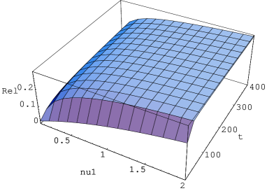
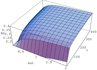
Fig. 7-a	Fig.7-b

Figure 7: Ratios $R_{el}\,=\,\sigma_{el}/\sigma_{tot}$ and $R_{D}\,=\,(\sigma_{el}+\sigma_{SD}+\sigma_{DD})/\sigma_{tot}$ versus $\nu_{1}$ and $t$, where $t$ is defined as $\nu_{2}\,=\,t\,\,\nu_{1}$.

In Fig.8 we take $t$ = 300 and plot $R_{D}$ and $R_{el}$ versus $\nu_{1}$ . One can see that $R_{D}$ is a very smooth function,, while $R_{el}$ depends substantially on $\nu_{1}$. Such a behaviour reflects the experimental situation shown in Fig.4. We use the experimental data for $R_{el}$ given in Fig.4 to assign a definite value of $\nu_{1}$ for a definite value of energy. In particular, we find $\nu_{1}=0.25$ for $\sqrt{s}\,=\,640\,GeV$ and $\nu_{1}=0.5$ for $\sqrt{s}\,=\,1800\,GeV$ to give $R_{el}=0.187$ and $R_{el}=0.237$, respectively.

Comparing Fig.8a and Fig.8b we can see that $\beta$ - dependence for $\beta\,>\,0.5$ is not essential.

Fig. 8-a	Fig.8-b

Figure 8: Ratios $R_{el}\,=\,\sigma_{el}/\sigma_{tot}$ and $R_{D}\,=\,(\sigma_{el}+\sigma_{SD}+\sigma_{DD})/\sigma_{tot}$ versus $\nu_{1}$ for two values of $\beta$ ( $\beta$ = 0.65 ( Fig.8a ) and $\beta$ = 0.5 ( Fig.8b ).

3.3 “Hard” radii

Before calculating the value of the survival probability we discuss the values of the “hard” radii $\tilde{R}^{2}_{i,k}$. Fortunately, these can be determined directly from the experimental data on diffractive production of vector mesons in DIS[25] at HERA. The data show that this production depends differently on the momentum transfer for elastic ( see, for example, the process $\gamma^{*}+p\,\rightarrow\,\Psi+p$ in Fig. 9 ) and inelastic ( $\gamma^{*}+p\,\rightarrow\,\Psi+X$ in Fig.9 ) production. In the exponential parameterization, the $t$ - dependence are characterized by the slopes $B_{el}$ and $B_{in}$.

Experimentally, these slopes are $B_{el}\,\,=\,\,4\,GeV^{-2}$ and $B_{in}\,\,=\,\,1.66\,GeV^{-2}$. Since the vertex $\gamma^{*}\,\rightarrow\,\Psi$ does not depend on $t$ at large value of photon virtuality $Q^{2}$, we can view such an experiment as a way of measuring the $t$ - dependence of the Pomeron - hadron form factor, and/or the transition form factor of a hadron to a diffractive state, due to Pomeron exchange. Incorporating the experimental data on slopes in the expressions of the “hard” radii we find

$$\tilde{R}^{2}_{1,1}\,\,\,\,=\,\,\,\,16\,\,GeV^{-2}\,\,;$$

$$\tilde{R}^{2}_{1,2}\,\,\,\,=\,\,\,\,11.32\,\,GeV^{-2}\,\,;$$ (66)

$$\tilde{R}^{2}_{2,2}\,\,\,\,=\,\,\,\,6.64\,\,GeV^{-2}\,\,.$$

One can see from Eq. (63) the value of the survival probability depends on the ratios $r_{i,k}$. To calculate these ratios we have to specify the values of “soft” radii $R^{2}_{i,k}$. We assumed the following values for the “soft” radii

$$R^{2}_{1,1}\,\,\,\,=\,\,\,\,12\,\,\,+\,\,4\,\alpha^{\prime}_{P}(0)\,\,\ln(s/s_{0})\,\,GeV^{-2}\,\,;$$

$$R^{2}_{1,2}\,\,\,\,=\,\,\,6\,\,\,+\,\,4\,\alpha^{\prime}_{P}(0)\,\,\ln(s/s_{0})\,\,GeV^{-2}\,\,;$$ (67)

$$R^{2}_{2,2}\,\,\,\,=\,\,\,\,4\,\alpha^{\prime}_{P}\,\ln(s/s_{0})\,\,GeV^{-2}\,\,.$$

It should be stressed that these radii are taken from our parameterization of the “soft” data, but they also describe the data on the elastic slope, and agree with known information on the $t$ - dependence of single diffraction dissociation[23].

Figure 9: Two slopes in diffractive J/$\Psi$ production in DIS in the Additive Quark Model.

3.4 $\mathbf{<\mid S^{2}_{spectator}(\,s\,)\mid>}$

In Fig.10 ( solid curve ) we show the value of the survival probability at $\sqrt{s}\,\,=\,\,1800\,GeV$ as a function of $\beta$. This value turns out to be rather small, in agreement with the experimental data[13].

Fig.11 ( solid curve ) shows the energy dependence of $<\mid S^{2}_{spectator}(\,s\,)\mid^{2}>$, namely the ratio

$$R\,\,\,\,=\,\,\,\frac{<\mid S^{2}_{spectator}(\,\sqrt{s}\,=\,640\,\,GeV\,)\mid^{2}>}{<\mid S^{2}_{spectator}(\,\sqrt{s}\,=\,1800\,\,GeV\,)\mid^{2}>}\,\,,$$ (68)

versus $\beta$.

In both these figures, at each fixed $\beta$, we found the values of $\nu_{1}$ for $\sqrt{s}=640\,GeV$ and for $\sqrt{s}=1800\,GeV$ from the values of $R_{el}$ ( $R_{el}\,=\,0.187$ and $R_{el}\,=\,0.237$, respectively, see Fig.4a ). The value of the survival probability was calculated using Eq. (63).

One can see that the ratio $R_{S}$ reaches the value of 2.2 for $\beta=0.6$, which we consider a typical value which fits the experimental data. It should be stressed that for $\beta\,<\,0.5$ the value of $R_{D}$ is smaller than 0.3. This fact is in contradiction with the experimental data shown in Fig.4b. At $\beta=0$ we reduce to the usual Eikonal Model and we obtain a ratio $R_{S}$ which is about 1.6. In Ref.[11] we found a larger value as we used an average value for the “hard” radius, while here we have introduced different radii for the different processes.

We would like to stress, that the accuracy of our estimates is not high. This is mostly because of the large dispersion of the experimental data for $R_{el}$ ( see Fig.4a ). To illustrate this point we plot the value of $<\mid S^{2}\mid>$ in Fig.10 ( dotted line ) taking $R_{el}$ = 0.215 at $\sqrt{s}=1800\,GeV$. One can see that the difference between these two curve is about a factor of 2. The spread of the experimental data influences dramatically the ratio of Eq. (68) ( see Fig.11 ). To illustrate it we plot in Fig.11 several lines that correspond to different choices of $R_{el}$

$$R_{el}(\sqrt{s}\,=\,640\,GeV)\,\,=\,\,0.187\,\,\,and\,\,\,R_{el}(\sqrt{s}\,=\,1800\,GeV)\,\,=\,\,0.237\,\,;$$ (69)

$$R_{el}(\sqrt{s}\,=\,640\,GeV)\,\,=\,\,0.212\,\,\,and\,\,\,R_{el}(\sqrt{s}\,=\,1800\,GeV)\,\,=\,\,0.237\,\,;$$ (70)

$$R_{el}(\sqrt{s}\,=\,640\,GeV)\,\,=\,\,0.187\,\,\,and\,\,\,R_{el}(\sqrt{s}\,=\,1800\,GeV)\,\,=\,\,0.215\,\,.$$ (71)

The full line in Fig.11 corresponds to parameters of Eq. (69), the dashed line to parameters of Eq. (70) and the dash-dotted line to parameters of Eq. (71).

We conclude, therefore, that we cannot obtain a definite prediction even within the framework of a particular model, due to the uncertainties in the experimental data on $R_{el}$.

Figure 10: The value of $<\mid S^{2}\mid>$ at $\sqrt{s}=W=1800GeV$ versus $\beta$ in the three channel model. The full and dashed lines corresponds to parameters of Eq. (69) and Eq. (70), respectively.

Figure 11: The value of ratio $<\mid S^{2}\mid>(W=640\,GeV)/<\mid S^{2}\mid>(W=1800\,GeV)$ versus $\beta$ in the three channel model. W = $\sqrt{s}$.The full, dashed and dash-dotted lines corresponds to parameters of Eq. (69), Eq. (70) and Eq. (71), respectively

4 Discussion and Summary

In this paper we give an example of a model in which

1. The processes of elastic and diffractive rescatterings have been taken into account, their cross sections being of the same order of magnitude ( $\sigma_{SD}\,\approx\sigma_{el}$ and $\sigma_{DD}\,\approx\,\sigma_{el}$ )  ;

2. It was shown that the scale of the SC is not given by the ratio $R_{D}$, but rather by the separate ratios $\sigma_{el}/\sigma_{tot}$, $\sigma_{SD}/\sigma_{tot}$ and $\sigma_{DD}/\sigma_{tot}$. Since each of these ratios shows considerable energy dependence, we do not expect a constant survival probability, contrary to the simpler model of Ref.[9];

3. It was demonstrated that the small value of the survival probability, as well as its strong energy dependence appear naturally in our approach;

4. The rather large value of $\nu_{2}\,\approx\,\,300\,\nu_{1}$ reflects (i) a smaller value of $R^{2}_{2,2}$ in comparison with $R^{2}_{1,1}$ observed experimentally, and (ii) the fact that this value takes into account the integration over the mass of the produced hadrons in our oversimplified model;

5. The parameters that have been used are in agreement with the more detailed fit of the experimental data on “soft” processes ( see Ref.[24] ).

Theoretical predictions for the value of the survival probability are still not very reliable. However, developing different models enables us to learn and assess which class of models provides natural predictions for both the value and the energy behaviour of the survival probability. We want to draw the readers attention to the fact that our estimates for the value of the survival probability given in Figs. 10 and 11 are very close to the estimates obtained in the Eikonal Model[11], in spite of the fact that the three channel model is quite different from the eikonal one.

New measurements both on LRG processes, and on the cross sections of diffraction dissociation ( in particular, on double diffraction ) would be very useful for a deeper understanding of “soft” interactions at high energy.

Acknowledgements: This research was supported in part by the Israel Science Foundation, founded by Israel Academy of Science and Humanities.

References

-
[1]
Yu. L. Dokshitzer, V. Khoze and S.I. Troyan, Proc.“Physics in
Collisions 6”, p. 417, ed. M. Derrick, WS 1987; Sov. J. Nucl.
Phys. 46, 712 (1987);
Yu. L. Dokshitzer, V. Khoze and T. Sjostrand, Phys. Lett. B274, 116 (1992). - [2] J. D. Bjorken, Int. J. Mod. Phys. A7, 4189 (1992); Phys. Rev. D47, 101 (1993).
- [3] E.A. Kuraev, L.N. Lipatov and V.S. Fadin, Sov. Phys. JETP 45, 199 (1977) ; Ya.Ya. Balitskii and L.V. Lipatov, Sov. J. Nucl. Phys. 28, 822 (1978); L.N. Lipatov, Sov. Phys. JETP 63 904 (1986).
- [4] F. Low,Phys. Rev. D12, 163 (1975); S. Nussinov, Phys. Rev. Lett. 34, 1286 (1975), Phys. Rev. D14, 244 (1976).
- [5] V.A.Khoze, A.D.Martin, M.G.Ryskin,Phys.Lett. B401 , 330 (1997); Phys.Rev. D56, 5867 (1997); G. Oderda, G. Sterman, Phys. Rev. Lett. 81, 3591 (1998).
- [6] E. Gotsman, E.M. Levin and U. Maor,Phys. Lett. B309, 199 (1993).
- [7] E. Levin, Phys. Rev. D48, 2097 (1993).
- [8] R.S. Fletcher, Phys. Rev. D48, 5162 (1993).
- [9] A. Rostovtsev and M.G. Ryskin, Phys. Lett. B390, 375 (1997) .
- [10] E. Gotsman, E.M. Levin and U. Maor, Nucl. Phys. B493, 354 (1997).
- [11] E. Gotsman, E.M. Levin and U. Maor, Phys. Lett. B438, 229 (1998).
- [12] CDF Collaboration; F. Abe et al., Phys. Rev. Lett. 74, 855 (1995); 80, 1156 (1998); 81, 5278 (1998).
-
[13]
D0 Collaboration, S. Abachi et al., Phys. Rev. Lett. 72,
2332 (1994); Phys. Rev. Lett. 76, 734 (1994);
A. Brandt, “Proceedings of the 4th Workshop on Small-x and Diffractive Physics”,Sept. 17-20, 1998, FNAL,p.461. - [14] ZEUS collaboration, M. Derrick et al., Phys. Lett. B315, 481 (1993); Z. Phys. C68,569 (1995); Phys. Lett. B369, 55 (1996).
-
[15]
E.L. Feinberg, ZhETP 29, 115 (1955) ;
A. I. Akieser and A.G. Sitenko, ZhETP 32 , 744 (1957). - [16] M.L. Good and W.D. Walker, Phys. Rev. 120, 1857 (1960).
- [17] J. Pumplin, Phys. Rev. D8, 2899 (1973).
- [18] A. Donnachie and P.V. Landshoff, Nucl. Phys. B244, 322 (1984); Nucl. Phys. B267, 690 (1986), Phys. Lett. B296, 227 (1992); Z. Phys. C61, 139 (1994).
- [19] L.V. Gribov, E.M. Levin and M.G. Ryskin, Phys. Rep. 100, 1 (1983).
- [20] E. Gotsman, E. Levin and U. Maor, Phys.Lett. B425, 369 (1998); E. Gotsman, E. Levin, U. Maor and E. Naftali, DESY 98-102,TAUP 2515/98, hep-ph/9808257, Nucl. Phys. B ( in press ).
- [21] F. Abe et al.,CDF Collaboration, FERMILAB-PUB-97/083-E.
- [22] K.G. Boreskov, A. M. Lapidus, S.T. Sukhorukov and K.A. Ter-Martirosyan, Nucl. Phys. B40, 397 (1972); P.E. Volkovitsky and A.M. Lapidus, Sov. J. Nucl. Phys. 31, 380 (1980).
- [23] K. Goulianos, Phys. Rep. C101 , 169 (1983).
- [24] E. Gotsman, E. Levin and U. Maor, TAUP 2560 - 99, hep-ph/9901416.
-
[25]
S. Aid et al.,H1 Collaboration, Nucl. Phys. B472, 3 (1996);
M. Derrick et al., ZEUS Collaboration, Phys. Lett. B350, 120 (1996).