hep-ph/9902255 RIKEN-BNL preprint Investigating the origins of transverse spin asymmetries at RHIC

Abstract

We discuss possible origins of transverse spin asymmetries in hadron-hadron collisions and propose an explanation in terms of a chiral-odd T-odd distribution function with intrinsic transverse momentum dependence, which would signal a correlation between the transverse spin and the transverse momentum of quarks inside an unpolarized hadron. We will argue that despite its conceptual problems, it can account for single spin asymmetries, for example in $p\,p^{\uparrow}\rightarrow\pi\,X$, and at the same time for the large $\cos 2\phi$ asymmetry in the unpolarized Drell-Yan cross section, which still lacks understanding. We use the latter asymmetry to arrive at a crude model for this function and show explicitly how it relates unpolarized and polarized observables in the Drell-Yan process, as could be measured with the proton-proton collisions at RHIC. Moreover, it would provide an alternative method of accessing the transversity distribution function $h_{1}$. For future reference we also list the complete set of azimuthal asymmetries in the unpolarized and polarized Drell-Yan process at leading order involving T-odd distribution functions with intrinsic transverse momentum dependence.

13.88.+e; 13.85.Qk

I Introduction

Large single transverse spin asymmetries have been observed experimentally in the process $p\,p^{\uparrow}\rightarrow\pi\,X$ [1] and many theoretical studies have been devoted to explain the possible origin(s) of such asymmetries. However, one experiment cannot reveal the origin(s) conclusively and one needs comparison to other experiments. In this article we will use additional experimental results to propose an explanation in terms of a chiral-odd T-odd distribution function with intrinsic transverse momentum dependence and we contrast it to the more standard theoretical proposals (cf. [2]). In addition, it can account for the large $\cos 2\phi$ asymmetry in the unpolarized Drell-Yan cross section [3, 4], which still lacks understanding.

Unlike the chiral-even T-odd distribution function with intrinsic transverse momentum dependence as investigated by [5, 6], which depends on the polarization of the parent hadron, the chiral-odd function signals a correlation between the transverse spin and the transverse momentum of quarks inside an unpolarized hadron. But one can use the polarization of one hadron to become sensitive to the polarization of quarks in another, unpolarized hadron. In this way it could provide a new way of measuring the transversity distribution function $h_{1}$. We propose two measurements that could be done at RHIC using polarized proton-proton collisions to study such a mechanism and to try to obtain information on $h_{1}$.

Apart from discussing the advantages of this proposal, we will discuss the theoretical difficulties connected to such a function. The function is actually the distribution function analog of the fragmentation function associated with the Collins effect [7]. Unlike the fragmentation function the distribution function is expected to be zero due to time reversal symmetry, unless one assumes some nonstandard mechanism to generate such a function, like for instance factorization breaking, which implies non-universality, or effects due to the finite size of a hadron, in which case one has the problem of systematically taking into account such effects in hard scattering factorization.

The article is organized as follows. In Section II we discuss possible origins for transverse spin asymmetries. In Section III we elaborate on transverse momentum dependent distribution functions. In Section IV and also in the appendix, we give results for the leading order Drell-Yan cross section in terms of the T-odd distribution functions, for completeness taking into account contributions from Z-bosons. In Section V we discuss how one particular function can not only explain (in principle) the single spin asymmetries in the process $p\,p^{\uparrow}\rightarrow\pi\,X$, but also explain the azimuthal $\cos 2\phi$ dependence of the unpolarized Drell-Yan cross section data [3, 4]. In Section VI we propose the measurements that could be performed at RHIC and that might uncover such an underlying mechanism. In Section VII we discuss the conceptual and theoretical problems related to T-odd distribution functions.

II Origins of transverse spin asymmetries

We will discuss possible origins of transverse spin asymmetries in the context of the following hard scattering processes, that either have been or will be performed. First we will go into the details of the single and double polarized Drell-Yan process $H_{1}\,H_{2}\rightarrow\ell\,\bar{\ell}\,X$, for which there is no data available yet. Then we focus on the single polarized process $p\,p^{\uparrow}\rightarrow\pi\,X$ for which large single transverse spin asymmetries have been observed [1]. We will also make use of knowledge of the unpolarized processes: $\pi^{-}\,N\rightarrow\mu^{+}\,\mu^{-}\,X$ and $e^{+}\,e^{-}\rightarrow h_{1}\,h_{2}\,X$.

A The polarized Drell-Yan process

Transverse spin asymmetries in hadron-hadron collisions require an explanation that involves quarks and gluons. A large scale (the center of mass energy or the large lepton pair mass) allows for a factorization of such a process into parts describing the soft physics convoluted with an elementary cross section. The parts parametrizing the soft physics cannot be calculated within perturbative QCD. Let us first focus on the Drell-Yan process, i.e. lepton pair production in hadron-hadron collisions.

In lowest order, i.e. the parton model approximation, the Drell-Yan process consists of two soft parts (in Fig. 1 the leading order diagram is depicted [8]) and one of the soft parts is described by the quark correlation function $\Phi(P_{1},S_{1};p)$ and the other soft part by the antiquark correlation function, denoted by $\overline{\Phi}(P_{2},S_{2};k)$:

$$\Phi_{ij}(P_{1},S_{1};p) = \int\frac{d^{4}z}{(2\pi)^{4}}e^{ip\cdot z}\langle P_{1},S_{1}|\overline{\psi}_{j}(0)\psi_{i}(z)|P_{1},S_{1}\rangle,$$ (1)

$$\overline{\Phi}_{ij}(P_{2},S_{2};k) = \int\frac{d^{4}z}{(2\pi)^{4}}\,e^{-ik\cdot z}\langle P_{2},S_{2}|\psi_{i}(z)\overline{\psi}_{j}(0)|P_{2},S_{2}\rangle.$$ (2)

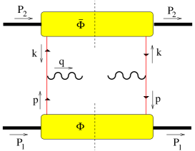
FIG. 1.: The leading order contribution to the Drell-Yan process

As will be discussed in the next section one can decompose the quark momenta $p$ and $k$ into parts that are along the direction of the parent hadron, the so-called lightcone momentum fractions, and deviations from that direction. In case one integrates over the transverse momentum of the lepton pair one only has to consider the correlation functions as functions of the lightcone momentum fractions.

The most general parametrization of the correlation function $\Phi$ as a function of the lightcone momentum fraction $x$, that is in accordance with the required symmetries (hermiticity, parity, time reversal), is given by:

$$\Phi(x)=\frac{1}{2}\left[{f_{1}(x)}\mbox{$\not\!P\,$}+{g_{1}(x)}\,\lambda\gamma_{5}\mbox{$\not\!P\,$}+{h_{1}(x)}\,\gamma_{5}\mbox{$\not\!S$}_{T}\mbox{$\not\!P\,$}\right].$$ (3)

Other common notation is $q$ for $f_{1}$, $\Delta q$ for $g_{1}$ and $\delta q$ or $\Delta_{T}q$ for $h_{1}$.

At this parton level one finds the well-known double transverse spin asymmetry [8],

$$A_{TT}\propto|\mathchoice{{\hbox{\boldmath$\displaystyle S$}}}{{\hbox{\boldmath$\textstyle S$}}}{{\hbox{\boldmath$\scriptstyle S$}}}{{\hbox{\boldmath$\scriptscriptstyle S$}}}_{1T}|\;|\mathchoice{{\hbox{\boldmath$\displaystyle S$}}}{{\hbox{\boldmath$\textstyle S$}}}{{\hbox{\boldmath$\scriptstyle S$}}}{{\hbox{\boldmath$\scriptscriptstyle S$}}}_{2T}|\;\cos(\phi_{S_{1}}+\phi_{S_{2}})\;h_{1}(x_{1})\,\overline{h}_{1}(x_{2}),$$ (4)

which has not yet been experimentally observed, but is one of the objectives of the polarized proton-proton scattering program to be performed at RHIC. This asymmetry is one of the possible ways to get information on the transversity distribution function $h_{1}$.

At the parton model level there are no single transverse spin asymmetries, but these might arise from corrections to this lowest order diagram. The corrections are of two types: the perturbative and the higher twist corrections. The first type depends logarithmically on the hard scale and the second type behaves as inverse powers of the hard scale.

Assuming that single spin asymmetries arise due to perturbative contributions is conceptually the simplest option, since it assumes that the asymmetries actually occur at the quark-gluon level, i.e. they arise from elementary subprocesses, and that going to the hadron level just involves convoluting the elementary asymmetry with (polarized) parton distributions. Typically this will yield single transverse spin asymmetries of the order $\alpha_{s}m_{q}/\sqrt{s}$ [9] which is expected to be small. The perturbative corrections to the double transverse spin asymmetry Eq. (4) have been calculated in [11] and using the assumption that at low energies the transversity distribution function $h_{1}$ equals the helicity distribution function $g_{1}$, it has been shown in Ref. [12] that $A_{TT}$ is expected to be of the order of a percent at RHIC energies. We will view this as an indication that perturbative QCD contributions are most likely not the (main) origin of large transverse spin asymmetries.

Dynamical higher twist corrections to the parton model require expanding the correlation function $\Phi(x)$ to include contributions proportional to the hadronic scale (typically the hadron mass), since these will show up in the cross section suppressed by $1/Q$, where $Q$ is a hard scale. At leading order in $\alpha_{s}$, i.e. $(\alpha_{s})^{0}$, but at the order $1/Q$, one finds [13, 14] no single or double transverse spin asymmetries.

Hence, in order to produce a large single transverse spin asymmetry one needs some conceptually nontrivial mechanism, since regular perturbative and higher twist contributions appear to be either small or absent. Two such nontrivial mechanisms are the soft gluon/fermion poles suggested by Qiu and Sterman [16] and so-called time-reversal (T) odd distribution functions (cf. e.g. [17]). Both of these mechanisms could produce a single transverse spin asymmetry $A_{T}$ at order $1/Q$. Recently it has been shown [17] that their effects are identical in the Drell-Yan process, so in order to discriminate between them one must use other experiments as well. This asymmetry $A_{T}$ has been estimated to be of the order of a percent at HERA energies (820 GeV, fixed target) [18]. Let us remark that T-odd functions need not signal actual time reversal symmetry violation. We will discuss other options more extensively in the discussion at the end.

In order to arrive at a single transverse spin asymmetry that is not suppressed by inverse powers of the hard scale, one can consider cross sections differential in the transverse momentum of the lepton pair. In that case one is sensitive to the transverse momentum of the quarks directly and in case this concerns intrinsic transverse momentum of the quarks inside a hadron, the effects need not be suppressed by $1/Q$. The point is that if the transverse momentum of the lepton pair is produced by perturbative QCD corrections, each factor of transverse momentum has to be accompanied by the inverse scale in the elementary hard scattering subprocess, that is by $1/Q$. But in case of intrinsic transverse momentum the relevant scale is not $Q$, but the hadronic scale, say the mass of the hadron. In processes with two (or more) soft parts, like the Drell-Yan process, the intrinsic transverse momentum of one soft part is linked to that of the other soft part resulting in effects, e.g. azimuthal asymmetries, not suppressed by $1/Q$. These effects will show up at relatively low (including nonperturbative) values of $Q_{T}$, where $Q_{T}^{2}=\mathchoice{{\hbox{\boldmath$\displaystyle q$}}}{{\hbox{\boldmath$\textstyle q$}}}{{\hbox{\boldmath$\scriptstyle q$}}}{{\hbox{\boldmath$\scriptscriptstyle q$}}}_{T}^{2}$ and $\mathchoice{{\hbox{\boldmath$\displaystyle q$}}}{{\hbox{\boldmath$\textstyle q$}}}{{\hbox{\boldmath$\scriptstyle q$}}}{{\hbox{\boldmath$\scriptscriptstyle q$}}}_{T}$ is the transverse momentum of the lepton pair. Studying the dependence of asymmetries on transverse momentum is another way to try to discriminate between possible origins for asymmetries.

Returning to the parton model diagram and including intrinsic transverse momentum dependence in this picture, one observes the following points. The effects will only show up if $Q_{T}$ is observed (i.e. not integrated over). If only T-even structures are included, several double spin azimuthal asymmetries are obtained, but no single spin asymmetries [14]. So again one needs to include some nontrivial mechanism. Gluonic and fermionic poles have as yet not been considered with transverse momentum dependence (other than perturbatively produced), but would in any case appear in the cross section suppressed by a factor of $1/Q$. However, the leading twist T-odd distribution functions with intrinsic transverse momentum dependence do yield single spin azimuthal asymmetries. We will be mainly focusing on the effects of such functions from now on.

B Pion production in $p\,p^{\uparrow}$ scattering

The large single transverse spin asymmetries that have been observed in the process $p\,p^{\uparrow}\rightarrow\pi\,X$ [1] require as said an explanation that involves quarks and gluons. Again one needs large scales (in this case also a large transverse momentum of the pion) to allow for a factorization of this process into parts describing the soft physics convoluted with an elementary cross section. For example, one contribution is coming from the diagram depicted in Fig. 2.

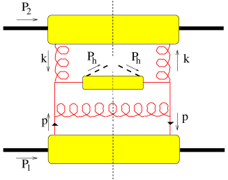
FIG. 2.: A contribution to the process $p\,p^{\uparrow}\rightarrow\pi\,X$

Assuming (as argued above) that perturbative and higher twist corrections (gluonic and fermionic pole contributions to this process have recently been investigated in Ref. [19]) are too small to generate the observed, large single transverse spin asymmetries, we will restrict ourselves to the transverse momentum dependent T-odd functions, in this case both distribution and fragmentation functions. The so-called Sivers [5] and Collins [7] effects are examples of transverse momentum dependent T-odd distribution and fragmentation functions, respectively. Like the transverse momentum of the lepton pair in the Drell-Yan process, the transverse momentum of the pion now originates from the intrinsic transverse momentum of the initial partons in addition to transverse momentum perturbatively generated by radiating off some additional parton(s) in the final state.

Anselmino et al. [6] have investigated both the Sivers and the Collins effect as possible origins for the asymmetries as observed in Ref. [1]. Both effects can be used to fit the data, which then can be tested using other observables. However, there are indications [20] from analyzing a particular angular dependence (a $\cos 2\phi$ dependence [21]) in the unpolarized process $e^{+}\,e^{-}\rightarrow Z^{0}\rightarrow\pi\,\pi\,X$, where the pions belong to opposite jets, that the Collins effect, is in fact at most a few percent of the magnitude of the ordinary unpolarized fragmentation function. Therefore, it seems unlikely that the Collins effect is the main source of the single spin asymmetries of the $p\,p^{\uparrow}\rightarrow\pi\,X$ process.

One other possible T-odd function that could be the source of the single spin asymmetries is the chiral-odd function $h_{1}^{\perp}$, the distribution function analog of the Collins effect. It will be discussed extensively below for the case of the Drell-Yan process, but it can equally well be the source of single spin asymmetries in $p\,p^{\uparrow}\rightarrow\pi\,X$. On the other hand, the Collins effect itself will not contribute to the Drell-Yan process.

C The unpolarized Drell-Yan process

The unpolarized cross section as measured for the process $\pi^{-}\,N\rightarrow\mu^{+}\,\mu^{-}\,X$, where $N$ is either deuterium or tungsten, using a $\pi^{-}$-beam with energy of 140, 194, 286 GeV [3] and 252 GeV [4],

$$\frac{1}{\sigma}\frac{d\sigma}{d\Omega}=\frac{3}{4\pi}\,\frac{1}{\lambda+3}\,\left(1+\lambda\cos^{2}\theta+\mu\sin^{2}\theta\cos\phi+\frac{\nu}{2}\sin^{2}\theta\cos 2\phi\right),$$ (5)

shows remarkably large values of $\nu$. It has been shown [3, 22] that its magnitude cannot be explained by leading and next-to-leading order perturbative QCD corrections. A number of explanations have been put forward, like a higher twist effect [23, 24], which is the $1/Q^{2}$ term discussed by Berger and Brodsky [25]. In Ref. [23] the higher twist effect is modeled using a pion distribution amplitude and it seems to fall short in explaining the large values as found for $\nu$. This higher twist effect would not be related to single spin asymmetries.

In Ref. [22] factorization breaking correlations between the incoming quarks are assumed and modeled in order to account for the large $\cos 2\phi$ dependence. We will return to that extensively in section V. Another approach is put forward in Ref. [26] using coherent states. This can describe the $\cos 2\phi$ data, however, it fails to describe the function $\mu$ in a satisfactory manner.

From the point of view of transverse momentum dependent distribution functions such a large $\cos 2\phi$ azimuthal dependence can arise at leading order only from a product of two T-odd functions, in particular, only from the distribution function $h_{1}^{\perp}$.

We would like to mention the experimental observation that the $\cos 2\phi$ dependence as observed by the NA10 collaboration does not seem to show a strong dependence on $A$, i.e. there was no significant difference between the deuterium and tungsten targets. Hence, it is unlikely that it is in fact dominated by nuclear effects instead of effects associated purely to hadrons. Therefore, the unpolarized cross section as can be measured at RHIC is also likely to show a large $\cos 2\phi$ dependence, although replacing the pion by a proton will probably have a suppressing effect.

Hence, we conclude that although there exist, apart from the $h_{1}^{\perp}$ mechanism, several explanations of single spin asymmetries and also of the unpolarized $\cos 2\phi$ dependence in the Drell-Yan cross section, none of the approaches relate the two types of asymmetry and most of the effects are expected or found to be (too) small. Moreover, the effects should not only be large, they should also exhibit the right $Q_{T}$ behavior.

III Transverse momentum dependent distribution functions

In this section we will discuss the transverse momentum dependent distribution functions that are needed to find the expressions for the leading order unpolarized and polarized Drell-Yan process cross sections differential in the transverse momentum of the lepton pair.

We consider again Fig. 1. The momenta of the quarks, which annihilate into the photon with momentum $q$, are predominantly along the direction of the parent hadrons. One hadron momentum ($P_{1}$) is chosen to be along the lightlike direction given by the vector $n_{+}$ (apart from mass corrections). The second hadron with momentum $P_{2}$ is predominantly in the $n_{-}$ direction which satisfies $n_{+}\cdot n_{-}=1$, such that $P_{1}\cdot P_{2}={\cal O}(q^{2})$. We make the following Sudakov decompositions:

$$P_{1}^{\mu} \equiv \frac{Q}{x_{1}\sqrt{2}}\,n_{+}^{\mu}+\frac{x_{1}M_{1}^{2}}{Q\sqrt{2}}\,n_{-}^{\mu},$$ (6)

$$P_{2}^{\mu} \equiv \frac{x_{2}M_{2}^{2}}{Q\sqrt{2}}\,n_{+}^{\mu}+\frac{Q}{x_{2}\sqrt{2}}\,n_{-}^{\mu},$$ (7)

$$q^{\mu} \equiv \frac{Q}{\sqrt{2}}\,n_{+}^{\mu}+\frac{Q}{\sqrt{2}}\,n_{-}^{\mu}+q_{T}^{\mu},$$ (8)

for $Q_{T}^{2}\equiv-q_{T}^{2}\equiv\mathchoice{{\hbox{\boldmath$\displaystyle q$}}}{{\hbox{\boldmath$\textstyle q$}}}{{\hbox{\boldmath$\scriptstyle q$}}}{{\hbox{\boldmath$\scriptscriptstyle q$}}}_{T}^{2}\ll Q^{2}$. We will often refer to the $\pm$ components of a momentum $p$, which are defined as $p^{\pm}=p\cdot n_{\mp}$. Furthermore, we decompose the parton momenta $p,k$ and the spin vectors $S_{1},S_{2}$ of the two hadrons as

$$p \equiv \frac{xQ}{x_{1}\sqrt{2}}\,n_{+}+\frac{x_{1}(p^{2}+\mathchoice{{\hbox{\boldmath$\displaystyle p$}}}{{\hbox{\boldmath$\textstyle p$}}}{{\hbox{\boldmath$\scriptstyle p$}}}{{\hbox{\boldmath$\scriptscriptstyle p$}}}_{T}^{2})}{xQ\sqrt{2}}\,n_{-}+p_{T},$$ (9)

$$k \equiv \frac{\bar{x}Q}{x_{2}\sqrt{2}}\,n_{-}+\frac{x_{2}(k^{2}+\mathchoice{{\hbox{\boldmath$\displaystyle k$}}}{{\hbox{\boldmath$\textstyle k$}}}{{\hbox{\boldmath$\scriptstyle k$}}}{{\hbox{\boldmath$\scriptscriptstyle k$}}}_{T}^{2})}{\bar{x}Q\sqrt{2}}\,n_{+}+k_{T},$$ (10)

$$S_{1} \equiv \frac{\lambda_{1}Q}{x_{1}M_{1}\sqrt{2}}\,n_{+}-\frac{x_{1}\lambda_{1}M_{1}}{Q\sqrt{2}}\,n_{-}+S_{1T},$$ (11)

$$S_{2} \equiv \frac{\lambda_{2}Q}{x_{2}M_{2}\sqrt{2}}\,n_{-}-\frac{x_{2}\lambda_{2}M_{2}}{Q\sqrt{2}}\,n_{+}+S_{2T}.$$ (12)

The four-momentum conservation delta-function at the photon vertex is written as (neglecting $1/Q^{2}$ contributions)

$$\delta^{4}(q-k-p)=\delta(q^{+}-p^{+})\,\delta(q^{-}-k^{-})\,\delta^{2}(\mathchoice{{\hbox{\boldmath$\displaystyle p$}}}{{\hbox{\boldmath$\textstyle p$}}}{{\hbox{\boldmath$\scriptstyle p$}}}{{\hbox{\boldmath$\scriptscriptstyle p$}}}_{T}+\mathchoice{{\hbox{\boldmath$\displaystyle k$}}}{{\hbox{\boldmath$\textstyle k$}}}{{\hbox{\boldmath$\scriptstyle k$}}}{{\hbox{\boldmath$\scriptscriptstyle k$}}}_{T}-\mathchoice{{\hbox{\boldmath$\displaystyle q$}}}{{\hbox{\boldmath$\textstyle q$}}}{{\hbox{\boldmath$\scriptstyle q$}}}{{\hbox{\boldmath$\scriptscriptstyle q$}}}_{T}),$$ (13)

fixing $xP_{1}^{+}=p^{+}=q^{+}=x_{1}P_{1}^{+}$, i.e., $x=x_{1}$ and similarly $\bar{x}=x_{2}$, and allows up to $1/Q^{2}$ corrections for integration over $p^{-}$ and $k^{+}$. However, the transverse momentum integrations cannot be separated, unless one integrates over the transverse momentum of the photon or equivalently of the lepton pair.

The parametrization of $\Phi(p)$ should be consistent with requirements imposed on $\Phi$ following from hermiticity, parity and time reversal invariance. The latter is normally taken to impose the following constraint on the correlation function [7, 14]

$$\Phi^{\ast}(P,S;p)=\gamma_{5}C\,\Phi(\bar{P},\bar{S};\bar{p})\,C^{\dagger}\gamma_{5}$$ (14)

where $\bar{p}$ = $(p^{0},-\mathchoice{{\hbox{\boldmath$\displaystyle p$}}}{{\hbox{\boldmath$\textstyle p$}}}{{\hbox{\boldmath$\scriptstyle p$}}}{{\hbox{\boldmath$\scriptscriptstyle p$}}})$, etc. For the validity of Eq. (14) it is essential that the incoming hadron is a plane wave state. We will not apply this constraint and in the last section we will discuss this issue in detail.

In the calculation in leading order we encounter the correlation function integrated over $p^{-}$, which is parametrized in terms of the transverse momentum dependent distribution functions as [27]

$$\Phi(x_{1},\mathchoice{{\hbox{\boldmath$\displaystyle p$}}}{{\hbox{\boldmath$\textstyle p$}}}{{\hbox{\boldmath$\scriptstyle p$}}}{{\hbox{\boldmath$\scriptscriptstyle p$}}}_{T}) \equiv \left.\int dp^{-}\ \Phi(P_{1},S_{1};p)\right|_{p^{+}=x_{1}P_{1}^{+},\mathchoice{{\hbox{\boldmath$\displaystyle p$}}}{{\hbox{\boldmath$\textstyle p$}}}{{\hbox{\boldmath$\scriptstyle p$}}}{{\hbox{\boldmath$\scriptscriptstyle p$}}}_{T}}=\frac{M_{1}}{2P_{1}^{+}}\,\Biggl{\{}f_{1}(x_{1},\mathchoice{{\hbox{\boldmath$\displaystyle p$}}}{{\hbox{\boldmath$\textstyle p$}}}{{\hbox{\boldmath$\scriptstyle p$}}}{{\hbox{\boldmath$\scriptscriptstyle p$}}}_{T})\,\frac{\mbox{$\not\!\!P_{1}$}}{M_{1}}+f_{1T}^{\perp}(x_{1},\mathchoice{{\hbox{\boldmath$\displaystyle p$}}}{{\hbox{\boldmath$\textstyle p$}}}{{\hbox{\boldmath$\scriptstyle p$}}}{{\hbox{\boldmath$\scriptscriptstyle p$}}}_{T})\,\epsilon_{\mu\nu\rho\sigma}\gamma^{\mu}\frac{P_{1}^{\nu}p_{T}^{\rho}S_{1T}^{\sigma}}{M_{1}^{2}}$$ (15)

$$-g_{1s}(x_{1},\mathchoice{{\hbox{\boldmath$\displaystyle p$}}}{{\hbox{\boldmath$\textstyle p$}}}{{\hbox{\boldmath$\scriptstyle p$}}}{{\hbox{\boldmath$\scriptscriptstyle p$}}}_{T})\,\frac{\mbox{$\not\!\!P_{1}$}\gamma_{5}}{M_{1}}-h_{1T}(x_{1},\mathchoice{{\hbox{\boldmath$\displaystyle p$}}}{{\hbox{\boldmath$\textstyle p$}}}{{\hbox{\boldmath$\scriptstyle p$}}}{{\hbox{\boldmath$\scriptscriptstyle p$}}}_{T})\,\frac{i\sigma_{\mu\nu}\gamma_{5}S_{1T}^{\mu}P_{1}^{\nu}}{M_{1}}-h_{1s}^{\perp}(x_{1},\mathchoice{{\hbox{\boldmath$\displaystyle p$}}}{{\hbox{\boldmath$\textstyle p$}}}{{\hbox{\boldmath$\scriptstyle p$}}}{{\hbox{\boldmath$\scriptscriptstyle p$}}}_{T})\,\frac{i\sigma_{\mu\nu}\gamma_{5}p_{T}^{\mu}P_{1}^{\nu}}{M_{1}^{2}}+h_{1}^{\perp}(x_{1},\mathchoice{{\hbox{\boldmath$\displaystyle p$}}}{{\hbox{\boldmath$\textstyle p$}}}{{\hbox{\boldmath$\scriptstyle p$}}}{{\hbox{\boldmath$\scriptscriptstyle p$}}}_{T})\,\frac{\sigma_{\mu\nu}p_{T}^{\mu}P_{1}^{\nu}}{M_{1}^{2}}\Biggl{\}}.$$ (16)

We used the shorthand notation

$$g_{1s}(x_{1},\mathchoice{{\hbox{\boldmath$\displaystyle p$}}}{{\hbox{\boldmath$\textstyle p$}}}{{\hbox{\boldmath$\scriptstyle p$}}}{{\hbox{\boldmath$\scriptscriptstyle p$}}}_{T})\equiv\lambda_{1}\,g_{1L}(x_{1},\mathchoice{{\hbox{\boldmath$\displaystyle p$}}}{{\hbox{\boldmath$\textstyle p$}}}{{\hbox{\boldmath$\scriptstyle p$}}}{{\hbox{\boldmath$\scriptscriptstyle p$}}}_{T}^{2})+\frac{(\mathchoice{{\hbox{\boldmath$\displaystyle p$}}}{{\hbox{\boldmath$\textstyle p$}}}{{\hbox{\boldmath$\scriptstyle p$}}}{{\hbox{\boldmath$\scriptscriptstyle p$}}}_{T}\cdot\mathchoice{{\hbox{\boldmath$\displaystyle S$}}}{{\hbox{\boldmath$\textstyle S$}}}{{\hbox{\boldmath$\scriptstyle S$}}}{{\hbox{\boldmath$\scriptscriptstyle S$}}}_{1T})}{M_{1}}\,g_{1T}(x_{1},\mathchoice{{\hbox{\boldmath$\displaystyle p$}}}{{\hbox{\boldmath$\textstyle p$}}}{{\hbox{\boldmath$\scriptstyle p$}}}{{\hbox{\boldmath$\scriptscriptstyle p$}}}_{T}^{2})$$ (17)

and similarly for $h_{1s}^{\perp}$. The parametrization contains two T-odd functions, that would vanish if the constraint Eq. (14) would be applied, i.e. the Sivers effect function $f_{1T}^{\perp}$ and the analog of the Collins effect, $h_{1}^{\perp}$.

The parametrization of $\overline{\Phi}$ is

$$\overline{\Phi}(x_{2},\mathchoice{{\hbox{\boldmath$\displaystyle k$}}}{{\hbox{\boldmath$\textstyle k$}}}{{\hbox{\boldmath$\scriptstyle k$}}}{{\hbox{\boldmath$\scriptscriptstyle k$}}}_{T}) \equiv \left.\int dk^{+}\ \overline{\Phi}(P_{2},S_{2};k)\right|_{k^{-}=x_{2}P_{2}^{-},\mathchoice{{\hbox{\boldmath$\displaystyle k$}}}{{\hbox{\boldmath$\textstyle k$}}}{{\hbox{\boldmath$\scriptstyle k$}}}{{\hbox{\boldmath$\scriptscriptstyle k$}}}_{T}}=\frac{M_{2}}{2P_{2}^{-}}\,\Biggl{\{}\overline{f}_{1}(x_{2},\mathchoice{{\hbox{\boldmath$\displaystyle k$}}}{{\hbox{\boldmath$\textstyle k$}}}{{\hbox{\boldmath$\scriptstyle k$}}}{{\hbox{\boldmath$\scriptscriptstyle k$}}}_{T})\,\frac{\mbox{$\not\!\!P_{2}$}}{M_{2}}+\overline{f}_{1T}^{\perp}(x_{2},\mathchoice{{\hbox{\boldmath$\displaystyle k$}}}{{\hbox{\boldmath$\textstyle k$}}}{{\hbox{\boldmath$\scriptstyle k$}}}{{\hbox{\boldmath$\scriptscriptstyle k$}}}_{T})\,\epsilon_{\mu\nu\rho\sigma}\gamma^{\mu}\frac{P_{2}^{\nu}k_{T}^{\rho}S_{2T}^{\sigma}}{M_{2}^{2}}$$ (18)

$$+\overline{g}_{1s}(x_{2},\mathchoice{{\hbox{\boldmath$\displaystyle k$}}}{{\hbox{\boldmath$\textstyle k$}}}{{\hbox{\boldmath$\scriptstyle k$}}}{{\hbox{\boldmath$\scriptscriptstyle k$}}}_{T})\,\frac{\mbox{$\not\!\!P_{2}$}\gamma_{5}}{M_{2}}-\overline{h}_{1T}(x_{2},\mathchoice{{\hbox{\boldmath$\displaystyle k$}}}{{\hbox{\boldmath$\textstyle k$}}}{{\hbox{\boldmath$\scriptstyle k$}}}{{\hbox{\boldmath$\scriptscriptstyle k$}}}_{T})\,\frac{i\sigma_{\mu\nu}\gamma_{5}S_{2T}^{\mu}P_{2}^{\nu}}{M_{2}}-\overline{h}_{1s}^{\perp}(x_{2},\mathchoice{{\hbox{\boldmath$\displaystyle k$}}}{{\hbox{\boldmath$\textstyle k$}}}{{\hbox{\boldmath$\scriptstyle k$}}}{{\hbox{\boldmath$\scriptscriptstyle k$}}}_{T})\,\frac{i\sigma_{\mu\nu}\gamma_{5}k_{T}^{\mu}P_{2}^{\nu}}{M_{2}^{2}}+\overline{h}_{1}^{\perp}(x_{2},\mathchoice{{\hbox{\boldmath$\displaystyle k$}}}{{\hbox{\boldmath$\textstyle k$}}}{{\hbox{\boldmath$\scriptstyle k$}}}{{\hbox{\boldmath$\scriptscriptstyle k$}}}_{T})\,\frac{\sigma_{\mu\nu}k_{T}^{\mu}P_{2}^{\nu}}{M_{2}^{2}}\Biggl{\}}.$$ (19)

The Sivers effect function $f_{1T}^{\perp}$ has the interpretation of the distribution of an unpolarized quark with nonzero transverse momentum inside a transversely polarized nucleon, while the function $h_{1}^{\perp}$ is interpreted as the distribution of a transversely polarized quark with nonzero transverse momentum inside an unpolarized hadron. In both cases the polarization is orthogonal to the transverse momentum of the quark.

In terms of these functions we can schematically say that in order to fit the $p\,p^{\uparrow}\rightarrow\pi\,X$ data, Anselmino et al. [6] consider the following options for the product of three functions that are parametrizing the three soft parts: $f_{1T}^{\perp}(x_{1},\mathchoice{{\hbox{\boldmath$\displaystyle p$}}}{{\hbox{\boldmath$\textstyle p$}}}{{\hbox{\boldmath$\scriptstyle p$}}}{{\hbox{\boldmath$\scriptscriptstyle p$}}}_{T})\overline{f}_{1}(x_{2})D_{1}(z)$ and $h_{1}(x_{1})\overline{f}_{1}(x_{2})H_{1}^{\perp}(z,\mathchoice{{\hbox{\boldmath$\displaystyle k$}}}{{\hbox{\boldmath$\textstyle k$}}}{{\hbox{\boldmath$\scriptstyle k$}}}{{\hbox{\boldmath$\scriptscriptstyle k$}}}_{T})$, where $\overline{f}_{1}(x_{2})$ (or $D_{1}(z)$) can be the gluon distribution (or fragmentation) function $g(x_{2})$ (or $G(z)$) instead also. However, there is one remaining option (for pion production), that we are advocating as a source of single spin asymmetries: $h_{1}^{\perp}(x_{1},\mathchoice{{\hbox{\boldmath$\displaystyle p$}}}{{\hbox{\boldmath$\textstyle p$}}}{{\hbox{\boldmath$\scriptstyle p$}}}{{\hbox{\boldmath$\scriptscriptstyle p$}}}_{T})\overline{h}_{1}(x_{2})D_{1}(z)$. Because of the appearance of two chiral-odd quantities this contribution might be expected to be smaller than $f_{1T}^{\perp}(x_{1},\mathchoice{{\hbox{\boldmath$\displaystyle p$}}}{{\hbox{\boldmath$\textstyle p$}}}{{\hbox{\boldmath$\scriptstyle p$}}}{{\hbox{\boldmath$\scriptscriptstyle p$}}}_{T})\overline{f}_{1}(x_{2})D_{1}(z)$. But even though $f_{1}\geq h_{1}$, one cannot exclude that $h_{1}^{\perp}(x_{1},\mathchoice{{\hbox{\boldmath$\displaystyle p$}}}{{\hbox{\boldmath$\textstyle p$}}}{{\hbox{\boldmath$\scriptstyle p$}}}{{\hbox{\boldmath$\scriptscriptstyle p$}}}_{T})$ is larger than $f_{1T}^{\perp}(x_{1},\mathchoice{{\hbox{\boldmath$\displaystyle p$}}}{{\hbox{\boldmath$\textstyle p$}}}{{\hbox{\boldmath$\scriptstyle p$}}}{{\hbox{\boldmath$\scriptscriptstyle p$}}}_{T})$.

Note that the magnitude of the Collins effect fragmentation function $H_{1}^{\perp}(z,\mathchoice{{\hbox{\boldmath$\displaystyle k$}}}{{\hbox{\boldmath$\textstyle k$}}}{{\hbox{\boldmath$\scriptstyle k$}}}{{\hbox{\boldmath$\scriptscriptstyle k$}}}_{T})$ need not be related to the magnitude of $h_{1}^{\perp}(z,\mathchoice{{\hbox{\boldmath$\displaystyle k$}}}{{\hbox{\boldmath$\textstyle k$}}}{{\hbox{\boldmath$\scriptstyle k$}}}{{\hbox{\boldmath$\scriptscriptstyle k$}}}_{T})$. In contrast to the distribution function, the fragmentation function will receive contributions due to the final state interactions which are present between the produced hadron and the other particles produced in the fragmenting of a quark. This is also the reason a similar constraint like Eq. (14) does not apply to fragmentation correlation functions.

IV Unpolarized and single spin dependent cross sections

The Drell-Yan cross section is obtained by contracting the lepton tensor with the hadron tensor

$${\cal W}^{\mu\nu}=\frac{1}{3}\int dp^{-}dk^{+}d^{2}\mathchoice{{\hbox{\boldmath$\displaystyle p$}}}{{\hbox{\boldmath$\textstyle p$}}}{{\hbox{\boldmath$\scriptstyle p$}}}{{\hbox{\boldmath$\scriptscriptstyle p$}}}_{T}d^{2}\mathchoice{{\hbox{\boldmath$\displaystyle k$}}}{{\hbox{\boldmath$\textstyle k$}}}{{\hbox{\boldmath$\scriptstyle k$}}}{{\hbox{\boldmath$\scriptscriptstyle k$}}}_{T}\,\delta^{2}(\mathchoice{{\hbox{\boldmath$\displaystyle p$}}}{{\hbox{\boldmath$\textstyle p$}}}{{\hbox{\boldmath$\scriptstyle p$}}}{{\hbox{\boldmath$\scriptscriptstyle p$}}}_{T}+\mathchoice{{\hbox{\boldmath$\displaystyle k$}}}{{\hbox{\boldmath$\textstyle k$}}}{{\hbox{\boldmath$\scriptstyle k$}}}{{\hbox{\boldmath$\scriptscriptstyle k$}}}_{T}-\mathchoice{{\hbox{\boldmath$\displaystyle q$}}}{{\hbox{\boldmath$\textstyle q$}}}{{\hbox{\boldmath$\scriptstyle q$}}}{{\hbox{\boldmath$\scriptscriptstyle q$}}}_{T})\,\left.\text{Tr}\left(\Phi(p)\,V_{1}^{\mu}\,\overline{\Phi}(k)\,V_{2}^{\nu}\right)\right|_{p^{+},\,k^{-}}+\left(\begin{array}[]{c}q\leftrightarrow-q\\ \mu\leftrightarrow\nu\end{array}\right).$$ (20)

The vertices $V_{i}^{\mu}$ can be either the photon vertex $V^{\mu}=e\gamma^{\mu}$ or the $Z$-boson vertex $V^{\mu}=g_{V}\gamma^{\mu}+g_{A}\gamma_{5}\gamma^{\mu}$. The vector and axial-vector couplings to the $Z$ boson are given by:

$$g_{V}^{j} = T_{3}^{j}-2\,Q^{j}\,\sin^{2}\theta_{W},$$ (21)

$$g_{A}^{j} = T_{3}^{j},$$ (22)

where $Q^{j}$ denotes the charge and $T_{3}^{j}$ the weak isospin of particle $j$ (i.e., $T_{3}^{j}=+1/2$ for $j=u$ and $T_{3}^{j}=-1/2$ for $j=e^{-},d,s$). We find for the leading order unpolarized Drell-Yan cross section, taking into account both photon and $Z$-boson contributions,

$$\frac{d\sigma^{(0)}(h_{1}h_{2}\to\ell\bar{\ell}X)}{d\Omega dx_{1}dx_{2}d^{2}{\mathchoice{{\hbox{\boldmath$\displaystyle q$}}}{{\hbox{\boldmath$\textstyle q$}}}{{\hbox{\boldmath$\scriptstyle q$}}}{{\hbox{\boldmath$\scriptscriptstyle q$}}}_{T}}}=\frac{\alpha^{2}}{3Q^{2}}\;\sum_{a,\bar{a}}\;\Bigg{\{}K_{1}(y)\;{\cal F}\left[f_{1}\overline{f}_{1}\right]$$ (24)

$$\qquad+\left[K_{3}(y)\cos(2\phi)+K_{4}(y)\sin(2\phi)\right]\;{\cal F}\left[\left(2\,\mathchoice{{\hbox{\boldmath$\displaystyle\hat{h}$}}}{{\hbox{\boldmath$\textstyle\hat{h}$}}}{{\hbox{\boldmath$\scriptstyle\hat{h}$}}}{{\hbox{\boldmath$\scriptscriptstyle\hat{h}$}}}\!\cdot\!\mathchoice{{\hbox{\boldmath$\displaystyle p$}}}{{\hbox{\boldmath$\textstyle p$}}}{{\hbox{\boldmath$\scriptstyle p$}}}{{\hbox{\boldmath$\scriptscriptstyle p$}}}_{T}\,\,\mathchoice{{\hbox{\boldmath$\displaystyle\hat{h}$}}}{{\hbox{\boldmath$\textstyle\hat{h}$}}}{{\hbox{\boldmath$\scriptstyle\hat{h}$}}}{{\hbox{\boldmath$\scriptscriptstyle\hat{h}$}}}\!\cdot\!\mathchoice{{\hbox{\boldmath$\displaystyle k$}}}{{\hbox{\boldmath$\textstyle k$}}}{{\hbox{\boldmath$\scriptstyle k$}}}{{\hbox{\boldmath$\scriptscriptstyle k$}}}_{T}\,-\,\mathchoice{{\hbox{\boldmath$\displaystyle p$}}}{{\hbox{\boldmath$\textstyle p$}}}{{\hbox{\boldmath$\scriptstyle p$}}}{{\hbox{\boldmath$\scriptscriptstyle p$}}}_{T}\!\cdot\!\mathchoice{{\hbox{\boldmath$\displaystyle k$}}}{{\hbox{\boldmath$\textstyle k$}}}{{\hbox{\boldmath$\scriptstyle k$}}}{{\hbox{\boldmath$\scriptscriptstyle k$}}}_{T}\,\right)\frac{h_{1}^{\perp}\overline{h}_{1}^{\perp}}{M_{1}M_{2}}\right]\Bigg{\}}$$

and for the case where hadron one is polarized:

$$\frac{d\sigma^{(1)}(h_{1}h_{2}\to\ell\bar{\ell}X)}{d\Omega dx_{1}dx_{2}d^{2}{\mathchoice{{\hbox{\boldmath$\displaystyle q$}}}{{\hbox{\boldmath$\textstyle q$}}}{{\hbox{\boldmath$\scriptstyle q$}}}{{\hbox{\boldmath$\scriptscriptstyle q$}}}_{T}}}=\frac{\alpha^{2}}{3Q^{2}}\;\sum_{a,\bar{a}}\;\Bigg{\{}\ldots$$ (30)

$$\qquad-{\lambda_{1}}\;\left[K_{3}(y)\sin(2\phi)-K_{4}(y)\cos(2\phi)\right]\;{\cal F}\left[\left(2\,\mathchoice{{\hbox{\boldmath$\displaystyle\hat{h}$}}}{{\hbox{\boldmath$\textstyle\hat{h}$}}}{{\hbox{\boldmath$\scriptstyle\hat{h}$}}}{{\hbox{\boldmath$\scriptscriptstyle\hat{h}$}}}\!\cdot\!\mathchoice{{\hbox{\boldmath$\displaystyle p$}}}{{\hbox{\boldmath$\textstyle p$}}}{{\hbox{\boldmath$\scriptstyle p$}}}{{\hbox{\boldmath$\scriptscriptstyle p$}}}_{T}\,\,\mathchoice{{\hbox{\boldmath$\displaystyle\hat{h}$}}}{{\hbox{\boldmath$\textstyle\hat{h}$}}}{{\hbox{\boldmath$\scriptstyle\hat{h}$}}}{{\hbox{\boldmath$\scriptscriptstyle\hat{h}$}}}\!\cdot\!\mathchoice{{\hbox{\boldmath$\displaystyle k$}}}{{\hbox{\boldmath$\textstyle k$}}}{{\hbox{\boldmath$\scriptstyle k$}}}{{\hbox{\boldmath$\scriptscriptstyle k$}}}_{T}\,-\,\mathchoice{{\hbox{\boldmath$\displaystyle p$}}}{{\hbox{\boldmath$\textstyle p$}}}{{\hbox{\boldmath$\scriptstyle p$}}}{{\hbox{\boldmath$\scriptscriptstyle p$}}}_{T}\!\cdot\!\mathchoice{{\hbox{\boldmath$\displaystyle k$}}}{{\hbox{\boldmath$\textstyle k$}}}{{\hbox{\boldmath$\scriptstyle k$}}}{{\hbox{\boldmath$\scriptscriptstyle k$}}}_{T}\,\right)\frac{h_{1L}^{\perp}\overline{h}_{1}^{\perp}}{M_{1}M_{2}}\right]$$

$$\qquad+|\mathchoice{{\hbox{\boldmath$\displaystyle S$}}}{{\hbox{\boldmath$\textstyle S$}}}{{\hbox{\boldmath$\scriptstyle S$}}}{{\hbox{\boldmath$\scriptscriptstyle S$}}}_{1T}|\;K_{1}(y)\;\sin(\phi-\phi_{S_{1}})\;{\cal F}\left[\,\mathchoice{{\hbox{\boldmath$\displaystyle\hat{h}$}}}{{\hbox{\boldmath$\textstyle\hat{h}$}}}{{\hbox{\boldmath$\scriptstyle\hat{h}$}}}{{\hbox{\boldmath$\scriptscriptstyle\hat{h}$}}}\!\cdot\!\mathchoice{{\hbox{\boldmath$\displaystyle p$}}}{{\hbox{\boldmath$\textstyle p$}}}{{\hbox{\boldmath$\scriptstyle p$}}}{{\hbox{\boldmath$\scriptscriptstyle p$}}}_{T}\,\frac{f_{1T}^{\perp}\overline{f}_{1}}{M_{1}}\right]$$

$$\qquad-|\mathchoice{{\hbox{\boldmath$\displaystyle S$}}}{{\hbox{\boldmath$\textstyle S$}}}{{\hbox{\boldmath$\scriptstyle S$}}}{{\hbox{\boldmath$\scriptscriptstyle S$}}}_{1T}|\;\left[K_{3}(y)\sin(\phi+\phi_{S_{1}})-K_{4}(y)\cos(\phi+\phi_{S_{1}})\right]\;{\cal F}\left[\,\mathchoice{{\hbox{\boldmath$\displaystyle\hat{h}$}}}{{\hbox{\boldmath$\textstyle\hat{h}$}}}{{\hbox{\boldmath$\scriptstyle\hat{h}$}}}{{\hbox{\boldmath$\scriptscriptstyle\hat{h}$}}}\!\cdot\!\mathchoice{{\hbox{\boldmath$\displaystyle k$}}}{{\hbox{\boldmath$\textstyle k$}}}{{\hbox{\boldmath$\scriptstyle k$}}}{{\hbox{\boldmath$\scriptscriptstyle k$}}}_{T}\,\frac{h_{1}\overline{h}_{1}^{\perp}}{M_{2}}\right]$$

$$\qquad-|\mathchoice{{\hbox{\boldmath$\displaystyle S$}}}{{\hbox{\boldmath$\textstyle S$}}}{{\hbox{\boldmath$\scriptstyle S$}}}{{\hbox{\boldmath$\scriptscriptstyle S$}}}_{1T}|\;\left[K_{3}(y)\sin(3\phi-\phi_{S_{1}})-K_{4}(y)\cos(3\phi-\phi_{S_{1}})\right]\;$$

$$\hskip 142.26378pt\times{\cal F}\left[\left(4\,\mathchoice{{\hbox{\boldmath$\displaystyle\hat{h}$}}}{{\hbox{\boldmath$\textstyle\hat{h}$}}}{{\hbox{\boldmath$\scriptstyle\hat{h}$}}}{{\hbox{\boldmath$\scriptscriptstyle\hat{h}$}}}\!\cdot\!\mathchoice{{\hbox{\boldmath$\displaystyle k$}}}{{\hbox{\boldmath$\textstyle k$}}}{{\hbox{\boldmath$\scriptstyle k$}}}{{\hbox{\boldmath$\scriptscriptstyle k$}}}_{T}\,(\!\,\mathchoice{{\hbox{\boldmath$\displaystyle\hat{h}$}}}{{\hbox{\boldmath$\textstyle\hat{h}$}}}{{\hbox{\boldmath$\scriptstyle\hat{h}$}}}{{\hbox{\boldmath$\scriptscriptstyle\hat{h}$}}}\!\cdot\!\mathchoice{{\hbox{\boldmath$\displaystyle p$}}}{{\hbox{\boldmath$\textstyle p$}}}{{\hbox{\boldmath$\scriptstyle p$}}}{{\hbox{\boldmath$\scriptscriptstyle p$}}}_{T}\,\!)^{2}-2\,\mathchoice{{\hbox{\boldmath$\displaystyle\hat{h}$}}}{{\hbox{\boldmath$\textstyle\hat{h}$}}}{{\hbox{\boldmath$\scriptstyle\hat{h}$}}}{{\hbox{\boldmath$\scriptscriptstyle\hat{h}$}}}\!\cdot\!\mathchoice{{\hbox{\boldmath$\displaystyle p$}}}{{\hbox{\boldmath$\textstyle p$}}}{{\hbox{\boldmath$\scriptstyle p$}}}{{\hbox{\boldmath$\scriptscriptstyle p$}}}_{T}\,\,\mathchoice{{\hbox{\boldmath$\displaystyle p$}}}{{\hbox{\boldmath$\textstyle p$}}}{{\hbox{\boldmath$\scriptstyle p$}}}{{\hbox{\boldmath$\scriptscriptstyle p$}}}_{T}\!\cdot\!\mathchoice{{\hbox{\boldmath$\displaystyle k$}}}{{\hbox{\boldmath$\textstyle k$}}}{{\hbox{\boldmath$\scriptstyle k$}}}{{\hbox{\boldmath$\scriptscriptstyle k$}}}_{T}\,-\,\mathchoice{{\hbox{\boldmath$\displaystyle\hat{h}$}}}{{\hbox{\boldmath$\textstyle\hat{h}$}}}{{\hbox{\boldmath$\scriptstyle\hat{h}$}}}{{\hbox{\boldmath$\scriptscriptstyle\hat{h}$}}}\!\cdot\!\mathchoice{{\hbox{\boldmath$\displaystyle k$}}}{{\hbox{\boldmath$\textstyle k$}}}{{\hbox{\boldmath$\scriptstyle k$}}}{{\hbox{\boldmath$\scriptscriptstyle k$}}}_{T}\,\,\mathchoice{{\hbox{\boldmath$\displaystyle p$}}}{{\hbox{\boldmath$\textstyle p$}}}{{\hbox{\boldmath$\scriptstyle p$}}}{{\hbox{\boldmath$\scriptscriptstyle p$}}}_{T}^{2}\,\right)\frac{h_{1T}^{\perp}\overline{h}_{1}^{\perp}}{2M_{1}{}^{2}M_{2}}\right]\Bigg{\}},$$

where the ellipsis stand for the T-even–T-even structures (which for the contribution of the virtual photon are absent, cf. Ref. [14]). Let us list the various definitions appearing in these expressions. We have defined the following combinations of the couplings and $Z$-boson propagators:

$$K_{1}(y) = A(y)\left[e_{a}^{2}+2g_{V}^{l}e_{a}g_{V}^{a}\chi_{1}+c_{1}^{l}c_{1}^{a}\chi_{2}\right]-\frac{C(y)}{2}\left[2g_{A}^{l}e_{a}g_{A}^{a}\chi_{1}+c_{3}^{l}c_{3}^{a}\chi_{2}\right],$$ (31)

$$K_{2}(y) = A(y)\left[2g_{V}^{l}e_{a}g_{A}^{a}\chi_{1}+c_{1}^{l}c_{3}^{a}\chi_{2}\right]-\frac{C(y)}{2}\left[2g_{A}^{l}e_{a}g_{V}^{a}\chi_{1}+c_{3}^{l}c_{1}^{a}\chi_{2}\right],$$ (32)

$$K_{3}(y) = B(y)\left[e_{a}^{2}+2g_{V}^{l}e_{a}g_{V}^{a}\chi_{1}+c_{1}^{l}c_{2}^{a}\chi_{2}\right],$$ (33)

$$K_{4}(y) = B(y)\left[2g_{V}^{l}e_{a}g_{A}^{a}\chi_{3}\right],$$ (34)

which contain the combinations of the couplings

$$c_{1}^{j} = \left(g_{V}^{j}{}^{2}+g_{A}^{j}{}^{2}\right),$$ (35)

$$c_{2}^{j} = \left(g_{V}^{j}{}^{2}-g_{A}^{j}{}^{2}\right),\qquad\qquad j=\ell\;\;\mbox{or}\;\;a$$ (36)

$$c_{3}^{j} = 2g_{V}^{j}g_{A}^{j}.$$ (37)

The $Z$-boson propagator factors are given by

$$\chi_{1} = \frac{1}{\sin^{2}(2\theta_{W})}\,\frac{Q^{2}(Q^{2}-M_{Z}^{2})}{(Q^{2}-M_{Z}^{2})^{2}+\Gamma_{Z}^{2}M_{Z}^{2}},$$ (38)

$$\chi_{2} = \frac{1}{\sin^{2}(2\theta_{W})}\,\frac{Q^{2}}{Q^{2}-M_{Z}^{2}}\chi_{1},$$ (39)

$$\chi_{3} = \frac{-\Gamma_{Z}M_{Z}}{Q^{2}-M_{Z}^{2}}\chi_{1}.$$ (40)

The above is expressed in the so-called Collins-Soper frame [28], for which we chose the following sets of normalized vectors (for details see e.g. [17]):

$$\hat{t} \equiv q/Q,$$ (41)

$$\hat{z} \equiv \frac{x_{1}}{Q}\tilde{P_{1}}-\frac{x_{2}}{Q}\tilde{P_{2}},$$ (42)

$$\hat{h} \equiv q_{T}/Q_{T}=(q-x_{1}\,P_{1}-x_{2}\,P_{2})/Q_{T},$$ (43)

where $\tilde{P_{i}}\equiv P_{i}-q/(2x_{i})$, such that:

$$n_{+}^{\mu} = \frac{1}{\sqrt{2}}\left[\hat{t}^{\mu}+\hat{z}^{\mu}-\,\frac{Q_{T}}{Q}\hat{h}^{\mu}\right],$$ (44)

$$n_{-}^{\mu} = \frac{1}{\sqrt{2}}\left[\hat{t}^{\mu}-\hat{z}^{\mu}-\,\frac{Q_{T}}{Q}\,\hat{h}^{\mu}\right].$$ (45)

The azimuthal angles lie inside the plane orthogonal to $t$ and $z$. In particular, $d\Omega$ = $2dy\,d\phi^{l}$, where $\phi^{l}$ gives the orientation of $\hat{l}_{\perp}^{\mu}\equiv\left(g^{\mu\nu}-\hat{t}^{\mu}\hat{t}^{\nu}+\hat{z}^{\mu}\hat{z}^{\nu}\right)l_{\nu}$, the perpendicular part of the lepton momentum $l$; $\phi,\phi_{S_{i}}$ are the angles between $\mathchoice{{\hbox{\boldmath$\displaystyle\hat{h}$}}}{{\hbox{\boldmath$\textstyle\hat{h}$}}}{{\hbox{\boldmath$\scriptstyle\hat{h}$}}}{{\hbox{\boldmath$\scriptscriptstyle\hat{h}$}}},\mathchoice{{\hbox{\boldmath$\displaystyle S$}}}{{\hbox{\boldmath$\textstyle S$}}}{{\hbox{\boldmath$\scriptstyle S$}}}{{\hbox{\boldmath$\scriptscriptstyle S$}}}_{iT}$ and $\hat{l}_{\perp}$, respectively. In the cross sections we also encounter the following functions of $y=l^{-}/q^{-}$, which in the lepton center of mass frame equals $y=(1+\cos\theta)/2$, where $\theta$ is the angle of $\hat{z}$ with respect to the momentum of the outgoing lepton $l$ (cf. Fig. 3):

$$A(y) = \left(\frac{1}{2}-y+y^{2}\right)\stackrel{{\scriptstyle cm}}{{=}}\frac{1}{4}\left(1+\cos^{2}\theta\right),$$ (46)

$$B(y) = y\,(1-y)\stackrel{{\scriptstyle cm}}{{=}}\frac{1}{4}\sin^{2}\theta,$$ (47)

$$C(y) = (1-2y)\stackrel{{\scriptstyle cm}}{{=}}-\cos\theta.$$ (48)

Furthermore, we use the convolution notation (Ralston and Soper [8] use $I[...]$)

$${\cal F}\left[f\overline{f}\,\right]\equiv\;\int d^{2}\mathchoice{{\hbox{\boldmath$\displaystyle p$}}}{{\hbox{\boldmath$\textstyle p$}}}{{\hbox{\boldmath$\scriptstyle p$}}}{{\hbox{\boldmath$\scriptscriptstyle p$}}}_{T}\;d^{2}\mathchoice{{\hbox{\boldmath$\displaystyle k$}}}{{\hbox{\boldmath$\textstyle k$}}}{{\hbox{\boldmath$\scriptstyle k$}}}{{\hbox{\boldmath$\scriptscriptstyle k$}}}_{T}\;\delta^{2}(\mathchoice{{\hbox{\boldmath$\displaystyle p$}}}{{\hbox{\boldmath$\textstyle p$}}}{{\hbox{\boldmath$\scriptstyle p$}}}{{\hbox{\boldmath$\scriptscriptstyle p$}}}_{T}+\mathchoice{{\hbox{\boldmath$\displaystyle k$}}}{{\hbox{\boldmath$\textstyle k$}}}{{\hbox{\boldmath$\scriptstyle k$}}}{{\hbox{\boldmath$\scriptscriptstyle k$}}}_{T}-\mathchoice{{\hbox{\boldmath$\displaystyle q$}}}{{\hbox{\boldmath$\textstyle q$}}}{{\hbox{\boldmath$\scriptstyle q$}}}{{\hbox{\boldmath$\scriptscriptstyle q$}}}_{T})f^{a}(x_{1},\mathchoice{{\hbox{\boldmath$\displaystyle p$}}}{{\hbox{\boldmath$\textstyle p$}}}{{\hbox{\boldmath$\scriptstyle p$}}}{{\hbox{\boldmath$\scriptscriptstyle p$}}}_{T}^{2})\overline{f}{}^{a}(x_{2},\mathchoice{{\hbox{\boldmath$\displaystyle k$}}}{{\hbox{\boldmath$\textstyle k$}}}{{\hbox{\boldmath$\scriptstyle k$}}}{{\hbox{\boldmath$\scriptscriptstyle k$}}}_{T}^{2}),$$ (49)

where $a$ is the flavor index.

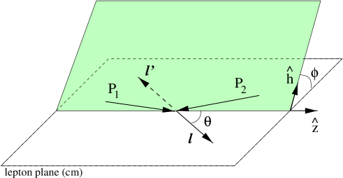
FIG. 3.: Kinematics of the Drell-Yan process in the lepton center of mass frame.

Since we are mainly concerned with the single polarized Drell-Yan process, we have given the double polarized cross section in the appendix for completeness and future reference.

V Quark spin correlations

In order to explain the angular dependence of the unpolarized cross section as measured for the process $\pi^{-}\,N\rightarrow\mu^{+}\,\mu^{-}\,X$, where $N$ is either deuterium or tungsten, using a $\pi^{-}$-beam with energy of 140, 194 and 286 GeV [3] ($-1/2<\cos\theta<1/2$), Brandenburg et al. [22] proposed factorization breaking correlations between the transverse momenta of the incoming quarks and between their transverse spins. This correlation between the transverse momenta is taken to be

$$P(\mathchoice{{\hbox{\boldmath$\displaystyle p$}}}{{\hbox{\boldmath$\textstyle p$}}}{{\hbox{\boldmath$\scriptstyle p$}}}{{\hbox{\boldmath$\scriptscriptstyle p$}}}_{T},\mathchoice{{\hbox{\boldmath$\displaystyle k$}}}{{\hbox{\boldmath$\textstyle k$}}}{{\hbox{\boldmath$\scriptstyle k$}}}{{\hbox{\boldmath$\scriptscriptstyle k$}}}_{T})\,d^{2}\mathchoice{{\hbox{\boldmath$\displaystyle p$}}}{{\hbox{\boldmath$\textstyle p$}}}{{\hbox{\boldmath$\scriptstyle p$}}}{{\hbox{\boldmath$\scriptscriptstyle p$}}}_{T}\,d^{2}\mathchoice{{\hbox{\boldmath$\displaystyle k$}}}{{\hbox{\boldmath$\textstyle k$}}}{{\hbox{\boldmath$\scriptstyle k$}}}{{\hbox{\boldmath$\scriptscriptstyle k$}}}_{T}=\frac{\alpha_{T}(\alpha_{T}+2\beta_{T})}{\pi^{2}}\,\exp\left[-\alpha_{T}(\mathchoice{{\hbox{\boldmath$\displaystyle p$}}}{{\hbox{\boldmath$\textstyle p$}}}{{\hbox{\boldmath$\scriptstyle p$}}}{{\hbox{\boldmath$\scriptscriptstyle p$}}}_{T}^{2}+\mathchoice{{\hbox{\boldmath$\displaystyle k$}}}{{\hbox{\boldmath$\textstyle k$}}}{{\hbox{\boldmath$\scriptstyle k$}}}{{\hbox{\boldmath$\scriptscriptstyle k$}}}_{T}^{2})-\beta_{T}(\mathchoice{{\hbox{\boldmath$\displaystyle p$}}}{{\hbox{\boldmath$\textstyle p$}}}{{\hbox{\boldmath$\scriptstyle p$}}}{{\hbox{\boldmath$\scriptscriptstyle p$}}}_{T}-\mathchoice{{\hbox{\boldmath$\displaystyle k$}}}{{\hbox{\boldmath$\textstyle k$}}}{{\hbox{\boldmath$\scriptstyle k$}}}{{\hbox{\boldmath$\scriptscriptstyle k$}}}_{T})^{2}\right]\,d^{2}\mathchoice{{\hbox{\boldmath$\displaystyle p$}}}{{\hbox{\boldmath$\textstyle p$}}}{{\hbox{\boldmath$\scriptstyle p$}}}{{\hbox{\boldmath$\scriptscriptstyle p$}}}_{T}\,d^{2}\mathchoice{{\hbox{\boldmath$\displaystyle k$}}}{{\hbox{\boldmath$\textstyle k$}}}{{\hbox{\boldmath$\scriptstyle k$}}}{{\hbox{\boldmath$\scriptscriptstyle k$}}}_{T},$$ (50)

which reduces to separate Gaussian transverse momentum dependences, since $\beta_{T}$ is found to be practically zero (and $\alpha_{T}=1\,\text{GeV}^{-2}$ at these energies).

In case the boson $V$ that produces the lepton pair, is a virtual photon ($V=\gamma^{*}$) Brandenburg et al. fit the cross section Eq. (5) using the data for the $\pi^{-}$-beam with energy of 194 GeV and lepton pair mass $m_{\gamma^{*}}=8\,\,\text{GeV}/c^{2}$. They find that $1-\lambda-2\nu\approx-4\kappa$, where they take the following model for $\kappa$, which is a measure of the correlation between the transverse spins of the incoming quarks,

$$\kappa=\kappa_{0}\,\frac{Q_{T}^{4}}{Q_{T}^{4}+m_{T}^{4}}$$ (51)

and the fitted values are $\kappa_{0}=0.17$ and $m_{T}=1.5$ GeV.

We will do a similar analysis based on the assumed presence of T-odd distribution functions with intrinsic transverse momentum dependence. For simplicity we take $\mu=0$, $\lambda=1$ (in accordance with the expectation from next-to-leading order perturbative QCD and the data in the Collins-Soper frame) and define $\nu=2\kappa$. For $V=\gamma^{*}$ we then find the following expression for $\kappa$ (cf. Eqs. (5) and (24)):

$$\kappa=\sum_{a,\bar{a}}e_{a}^{2}\,{\cal F}\left[\left(2\,\mathchoice{{\hbox{\boldmath$\displaystyle\hat{h}$}}}{{\hbox{\boldmath$\textstyle\hat{h}$}}}{{\hbox{\boldmath$\scriptstyle\hat{h}$}}}{{\hbox{\boldmath$\scriptscriptstyle\hat{h}$}}}\!\cdot\!\mathchoice{{\hbox{\boldmath$\displaystyle p$}}}{{\hbox{\boldmath$\textstyle p$}}}{{\hbox{\boldmath$\scriptstyle p$}}}{{\hbox{\boldmath$\scriptscriptstyle p$}}}_{T}\,\,\mathchoice{{\hbox{\boldmath$\displaystyle\hat{h}$}}}{{\hbox{\boldmath$\textstyle\hat{h}$}}}{{\hbox{\boldmath$\scriptstyle\hat{h}$}}}{{\hbox{\boldmath$\scriptscriptstyle\hat{h}$}}}\!\cdot\!\mathchoice{{\hbox{\boldmath$\displaystyle k$}}}{{\hbox{\boldmath$\textstyle k$}}}{{\hbox{\boldmath$\scriptstyle k$}}}{{\hbox{\boldmath$\scriptscriptstyle k$}}}_{T}\,-\,\mathchoice{{\hbox{\boldmath$\displaystyle p$}}}{{\hbox{\boldmath$\textstyle p$}}}{{\hbox{\boldmath$\scriptstyle p$}}}{{\hbox{\boldmath$\scriptscriptstyle p$}}}_{T}\!\cdot\!\mathchoice{{\hbox{\boldmath$\displaystyle k$}}}{{\hbox{\boldmath$\textstyle k$}}}{{\hbox{\boldmath$\scriptstyle k$}}}{{\hbox{\boldmath$\scriptscriptstyle k$}}}_{T}\,\right)\frac{h_{1}^{\perp}\overline{h}_{1}^{\perp}}{M_{1}M_{2}}\right]\Bigg{/}\sum_{a,\bar{a}}e_{a}^{2}\,{\cal F}\left[f_{1}\overline{f}_{1}\right].$$ (52)

A model for the shape of the function $h_{1}^{\perp}$ is needed. Collins’ parametrization [7] for the fragmentation function $H_{1}^{\perp}$ is (note that Collins uses the function $\Delta\hat{D}_{H/a}\sim\epsilon_{T}^{ij}s_{1Ti}k_{Tj}\,H_{1}^{\perp}$)

$$\frac{H_{1}^{\perp}(z,\mathchoice{{\hbox{\boldmath$\displaystyle k$}}}{{\hbox{\boldmath$\textstyle k$}}}{{\hbox{\boldmath$\scriptstyle k$}}}{{\hbox{\boldmath$\scriptscriptstyle k$}}}_{T}^{2})}{D_{1}(z,\mathchoice{{\hbox{\boldmath$\displaystyle k$}}}{{\hbox{\boldmath$\textstyle k$}}}{{\hbox{\boldmath$\scriptstyle k$}}}{{\hbox{\boldmath$\scriptscriptstyle k$}}}_{T}^{2})}=\frac{2M_{C}M_{h}}{\mathchoice{{\hbox{\boldmath$\displaystyle k$}}}{{\hbox{\boldmath$\textstyle k$}}}{{\hbox{\boldmath$\scriptstyle k$}}}{{\hbox{\boldmath$\scriptscriptstyle k$}}}_{T}^{2}+M_{C}^{2}}\,\text{Im}\left[A^{*}(k^{2})B(k^{2})\right]\,\frac{(1-z)}{z},$$ (53)

where $M_{h}$ is the mass of the produced hadron and in his model $M_{C}$ is the quark mass that appears in a dressed fermion propagator $i(A(k^{2})\mbox{$\not\!k$}+B(k^{2})M_{C})/(k^{2}-M_{C}^{2})$, the functions $A$ and $B$ are unity at $k^{2}=M_{C}^{2}$.

We assume a similar form for $h_{1}^{\perp}$ in terms of $f_{1}$ (we assume no flavor dependence of $M_{C}$):

$$\frac{h_{1}^{\perp}{}^{a}(x,\mathchoice{{\hbox{\boldmath$\displaystyle p$}}}{{\hbox{\boldmath$\textstyle p$}}}{{\hbox{\boldmath$\scriptstyle p$}}}{{\hbox{\boldmath$\scriptscriptstyle p$}}}_{T}^{2})}{f_{1}^{a}(x,\mathchoice{{\hbox{\boldmath$\displaystyle p$}}}{{\hbox{\boldmath$\textstyle p$}}}{{\hbox{\boldmath$\scriptstyle p$}}}{{\hbox{\boldmath$\scriptscriptstyle p$}}}_{T}^{2})}=c_{H}^{a}\frac{M_{C}M_{H}}{\mathchoice{{\hbox{\boldmath$\displaystyle p$}}}{{\hbox{\boldmath$\textstyle p$}}}{{\hbox{\boldmath$\scriptstyle p$}}}{{\hbox{\boldmath$\scriptscriptstyle p$}}}_{T}^{2}+M_{C}^{2}},$$ (54)

using the constant $c_{H}^{a}$ (which in principle is a function of $x$) and $M_{C}$ as the fitting parameters now (and similarly for the antiquark distribution functions). We also assume the above given Gaussian transverse momentum dependence for $f_{1}(x,\mathchoice{{\hbox{\boldmath$\displaystyle p$}}}{{\hbox{\boldmath$\textstyle p$}}}{{\hbox{\boldmath$\scriptstyle p$}}}{{\hbox{\boldmath$\scriptscriptstyle p$}}}_{T}^{2})$. After multiplying Eq. (52) by a trivial factor $Q_{T}^{2}/Q_{T}^{2}$, using the $\mathchoice{{\hbox{\boldmath$\displaystyle k$}}}{{\hbox{\boldmath$\textstyle k$}}}{{\hbox{\boldmath$\scriptstyle k$}}}{{\hbox{\boldmath$\scriptscriptstyle k$}}}_{T}$ integration to eliminate the delta function and shifting the integration variable $\mathchoice{{\hbox{\boldmath$\displaystyle p$}}}{{\hbox{\boldmath$\textstyle p$}}}{{\hbox{\boldmath$\scriptstyle p$}}}{{\hbox{\boldmath$\scriptscriptstyle p$}}}_{T}\to\mathchoice{{\hbox{\boldmath$\displaystyle p$}}}{{\hbox{\boldmath$\textstyle p$}}}{{\hbox{\boldmath$\scriptstyle p$}}}{{\hbox{\boldmath$\scriptscriptstyle p$}}}_{T}^{\prime}=\mathchoice{{\hbox{\boldmath$\displaystyle p$}}}{{\hbox{\boldmath$\textstyle p$}}}{{\hbox{\boldmath$\scriptstyle p$}}}{{\hbox{\boldmath$\scriptscriptstyle p$}}}_{T}-{\scriptstyle{1\over 2}}\mathchoice{{\hbox{\boldmath$\displaystyle q$}}}{{\hbox{\boldmath$\textstyle q$}}}{{\hbox{\boldmath$\scriptstyle q$}}}{{\hbox{\boldmath$\scriptscriptstyle q$}}}_{T}$, one arrives at

$$\kappa=\frac{\kappa_{1}\,\alpha_{T}}{\pi}\,M_{C}^{2}\,Q_{T}^{2}\,\int d^{2}\mathchoice{{\hbox{\boldmath$\displaystyle p$}}}{{\hbox{\boldmath$\textstyle p$}}}{{\hbox{\boldmath$\scriptstyle p$}}}{{\hbox{\boldmath$\scriptscriptstyle p$}}}_{T}^{\prime}\,\left[\frac{1}{(\mathchoice{{\hbox{\boldmath$\displaystyle p$}}}{{\hbox{\boldmath$\textstyle p$}}}{{\hbox{\boldmath$\scriptstyle p$}}}{{\hbox{\boldmath$\scriptscriptstyle p$}}}_{T}^{\prime}+{\scriptstyle{1\over 2}}\mathchoice{{\hbox{\boldmath$\displaystyle q$}}}{{\hbox{\boldmath$\textstyle q$}}}{{\hbox{\boldmath$\scriptstyle q$}}}{{\hbox{\boldmath$\scriptscriptstyle q$}}}_{T})^{2}+M_{C}^{2}}\,\frac{1}{(\mathchoice{{\hbox{\boldmath$\displaystyle p$}}}{{\hbox{\boldmath$\textstyle p$}}}{{\hbox{\boldmath$\scriptstyle p$}}}{{\hbox{\boldmath$\scriptscriptstyle p$}}}_{T}^{\prime}-{\scriptstyle{1\over 2}}\mathchoice{{\hbox{\boldmath$\displaystyle q$}}}{{\hbox{\boldmath$\textstyle q$}}}{{\hbox{\boldmath$\scriptstyle q$}}}{{\hbox{\boldmath$\scriptscriptstyle q$}}}_{T})^{2}+M_{C}^{2}}\right]\,e^{-2\alpha_{T}\mathchoice{{\hbox{\boldmath$\displaystyle p$}}}{{\hbox{\boldmath$\textstyle p$}}}{{\hbox{\boldmath$\scriptstyle p$}}}{{\hbox{\boldmath$\scriptscriptstyle p$}}}_{T}^{\prime}{}^{2}},$$ (55)

where $\kappa_{1}=c_{H_{1}}c_{H_{2}}/2$ and for the moment we considered the one flavor case. We approximate this by taking $\mathchoice{{\hbox{\boldmath$\displaystyle p$}}}{{\hbox{\boldmath$\textstyle p$}}}{{\hbox{\boldmath$\scriptstyle p$}}}{{\hbox{\boldmath$\scriptscriptstyle p$}}}_{T}^{\prime}=0$ (where the exponential factor is largest) in the term between square brackets (this is valid for large enough values of $Q_{T}$, but the resulting expression also has the right $Q_{T}^{2}$ behavior as $Q_{T}\to 0$), this results in (reinstalling the flavor summation)

$$\kappa=8\,\frac{Q_{T}^{2}\,M_{C}^{2}}{({Q}_{T}^{2}+4\,M_{C}^{2})^{2}}\,\frac{\sum_{a,\bar{a}}e_{a}^{2}\,\kappa_{1}^{a}\,f_{1}^{a}(x_{1})\,\overline{f}{}_{1}^{a}(x_{2})}{\sum_{a,\bar{a}}e_{a}^{2}\,f_{1}^{a}(x_{1})\,\overline{f}{}_{1}^{a}(x_{2})}.$$ (56)

Let us for simplicity also assume $\kappa_{1}^{a}$ to be independent of the flavor and fit

$$\kappa=8\kappa_{1}\,\frac{Q_{T}^{2}\,M_{C}^{2}}{({Q}_{T}^{2}+4\,M_{C}^{2})^{2}}$$ (57)

to the data at 194 GeV of Ref. [3]. This does not give as good a fit (Fig. 4) as a factor of $Q_{T}^{4}$ in the numerator would give (for this particular set of data), but it can obviously reproduce the tendency. Moreover, it has the desired property that $\kappa$ vanishes in the limit of $Q_{T}\to\infty$, as opposed to Eq. (51). We find for the dressed quark mass $M_{C}$ a rather large value of $2.3\pm 0.5\,\text{GeV}$ compared to the chiral symmetry breaking scale, but one should not take the model too seriously and we have made several approximations.

FIG. 4.: Data from [3] at 194 GeV and fit (using Eq. (57)) to $\nu=2\kappa$ as a function of the transverse momentum $Q_{T}$ of the lepton pair. The fitted parameters are $M_{C}=2.3\pm 0.5\,\text{GeV}$ and $16\,\kappa_{1}=7\pm 2$.

We have chosen the data at 194 GeV of Ref. [3], because it has the smallest errors (the error in $Q_{T}$ is chosen to be the bin size). The fits to the three other available sets of data, namely at 140 and 286 GeV of Ref. [3] and at 252 GeV of Ref. [4], yield lower values of $M_{C}$ and $\kappa_{1}$ (on average a factor 2 smaller), hence, have a lower maximum (at a smaller value of $Q_{T}$) and are less broad. We take the above result as providing a rough upper bound.

Taking for simplicity $c_{\pi}^{a}=c_{N}^{a}=c_{H}^{a}$, we arrive at a (crude) model for the function $h_{1}^{\perp}(x_{1},\mathchoice{{\hbox{\boldmath$\displaystyle p$}}}{{\hbox{\boldmath$\textstyle p$}}}{{\hbox{\boldmath$\scriptstyle p$}}}{{\hbox{\boldmath$\scriptscriptstyle p$}}}_{T}^{2})$:

$$h_{1}^{\perp}{}^{a}(x,\mathchoice{{\hbox{\boldmath$\displaystyle p$}}}{{\hbox{\boldmath$\textstyle p$}}}{{\hbox{\boldmath$\scriptstyle p$}}}{{\hbox{\boldmath$\scriptscriptstyle p$}}}_{T}^{2})=\frac{\alpha_{T}}{\pi}\,c_{H}^{a}\,\frac{M_{C}M_{H}}{\mathchoice{{\hbox{\boldmath$\displaystyle p$}}}{{\hbox{\boldmath$\textstyle p$}}}{{\hbox{\boldmath$\scriptstyle p$}}}{{\hbox{\boldmath$\scriptscriptstyle p$}}}_{T}^{2}+M_{C}^{2}}\,e^{-\alpha_{T}\mathchoice{{\hbox{\boldmath$\displaystyle p$}}}{{\hbox{\boldmath$\textstyle p$}}}{{\hbox{\boldmath$\scriptstyle p$}}}{{\hbox{\boldmath$\scriptscriptstyle p$}}}_{T}^{2}}\,f_{1}(x),$$ (58)

with $M_{C}=2.3\,\text{GeV}$, $c_{H}^{a}=1$ and $\alpha_{T}=1\,\text{GeV}^{-2}$, which can be used to get rough estimates for other asymmetries. The factor $\alpha_{T}/\pi$ comes from the consistency requirement between the definitions of $f_{1}(x)$ and $f_{1}(x,\mathchoice{{\hbox{\boldmath$\displaystyle k$}}}{{\hbox{\boldmath$\textstyle k$}}}{{\hbox{\boldmath$\scriptstyle k$}}}{{\hbox{\boldmath$\scriptscriptstyle k$}}}_{T}^{2})$ with a Gaussian $\mathchoice{{\hbox{\boldmath$\displaystyle k$}}}{{\hbox{\boldmath$\textstyle k$}}}{{\hbox{\boldmath$\scriptstyle k$}}}{{\hbox{\boldmath$\scriptscriptstyle k$}}}_{T}^{2}$ dependence. In the next section we will discuss the relevant asymmetries for RHIC.

VI Implications for RHIC

From Eq. (30) we see that in case $V=\gamma^{*}$ and that when we neglect the “higher harmonic” term containing the $3\phi$ dependence, there are two single transverse spin azimuthal dependences, namely $\sin(\phi-\phi_{S_{1}})$ arising with the Sivers function $f_{1T}^{\perp}$ and $\sin(\phi+\phi_{S_{1}})$ arising with $h_{1}^{\perp}$.

To estimate the size of the $\sin(\phi-\phi_{S_{1}})$ term, one can use for instance one of the usual parametrizations of $f_{1}$ and the parametrization for $f_{1T}^{\perp}$ as found by [6]. To estimate the size of the $\sin(\phi+\phi_{S_{1}})$ term, one can use one of the models for $h_{1}$ [12, 29] or take the upper bound for $h_{1}$ that arises from Soffer’s inequality ($g_{1}$ is also well-known) and one can use a fit for $h_{1}^{\perp}$ from the unpolarized azimuthal $\cos 2\phi$ dependence of the cross section in $p\,p\rightarrow\ell\,\bar{\ell}\,X$, in a similar way as was done in the previous section.

Let us examine the $\sin(\phi+\phi_{S_{1}})$ dependence of the cross section with the above given model for $h_{1}^{\perp}$. The relevant expression for the cross section in the polarized case is given by (cf. Eq. (5) with $\mu=0$ and $\lambda=1$)

$$\frac{1}{\sigma}\frac{d\sigma}{d\Omega\;d\phi_{S_{1}}}\propto\left(1+\cos^{2}\theta+\kappa\;\sin^{2}\theta\cos 2\phi-\rho\;|\mathchoice{{\hbox{\boldmath$\displaystyle S$}}}{{\hbox{\boldmath$\textstyle S$}}}{{\hbox{\boldmath$\scriptstyle S$}}}{{\hbox{\boldmath$\scriptscriptstyle S$}}}_{1T}|\;\sin^{2}\theta\;\sin(\phi+\phi_{S_{1}})+\ldots\right),$$ (59)

where the ellipsis stand for the other angular dependences. The analyzing power $\rho$ is found to be (cf. Eq. (30))

$$\rho=\sum_{a,\bar{a}}e_{a}^{2}\,{\cal F}\left[\mathchoice{{\hbox{\boldmath$\displaystyle\hat{h}$}}}{{\hbox{\boldmath$\textstyle\hat{h}$}}}{{\hbox{\boldmath$\scriptstyle\hat{h}$}}}{{\hbox{\boldmath$\scriptscriptstyle\hat{h}$}}}\!\cdot\!\mathchoice{{\hbox{\boldmath$\displaystyle k$}}}{{\hbox{\boldmath$\textstyle k$}}}{{\hbox{\boldmath$\scriptstyle k$}}}{{\hbox{\boldmath$\scriptscriptstyle k$}}}_{T}\,\frac{h_{1}\overline{h}_{1}^{\perp}}{M_{2}}\right]\Bigg{/}\sum_{a,\bar{a}}e_{a}^{2}\,{\cal F}\left[f_{1}\overline{f}_{1}\right].$$ (60)

Using the above model Eq. (58) for $h_{1}^{\perp}$ and performing similar approximations as before, we arrive at:

$$\rho=\frac{2\,M_{C}\,Q_{T}}{Q_{T}^{2}+4\,M_{C}^{2}}\,\frac{\sum_{a,\bar{a}}e_{a}^{2}\,c_{H_{2}}^{a}\,h_{1}^{a}(x_{1})\,\overline{f}{}_{1}^{a}(x_{2})}{\sum_{a,\bar{a}}e_{a}^{2}\,f_{1}^{a}(x_{1})\,\overline{f}{}_{1}^{a}(x_{2})}=\frac{1}{2}\sqrt{\frac{\kappa}{\kappa_{\text{max}}}}\,\frac{\sum_{a,\bar{a}}e_{a}^{2}\,c_{H_{2}}^{a}\,h_{1}^{a}(x_{1})\,\overline{f}{}_{1}^{a}(x_{2})}{\sum_{a,\bar{a}}e_{a}^{2}\,f_{1}^{a}(x_{1})\,\overline{f}{}_{1}^{a}(x_{2})},$$ (61)

where $\kappa_{\text{max}}$ is the maximum value of $\kappa$, which is at $Q_{T}=2M_{C}$. A determination of $\rho,\kappa,h_{1}$ should be mutually consistent according to the above equation, if the underlying mechanism is indeed the one that is assumed here. The maximum value $\rho$ is also at $Q_{T}=2M_{C}$, which in the case of one flavor corresponds to $\rho_{\text{max}}=c_{H}\,h_{1}(x_{1})/(2f_{1}(x_{1}))\leq c_{H}/2\approx 1/2$. If $h_{1}$ is for instance an order of magnitude smaller than $f_{1}$, this would give an analyzing power for this single transverse spin azimuthal asymmetry at the percent level.

The above scheme entails many extrapolations and assumptions and prevents us from stating accurate estimates for the asymmetries. One problem comes from the fact that the fit in the previous section resulted from data of the process $\pi^{-}\,N\rightarrow\mu^{+}\,\mu^{-}\,X$, where $N$ is either deuterium or tungsten, so extrapolation to $p\,p\rightarrow\ell\,\bar{\ell}\,X$ is unclear. One might expect that the $\cos 2\phi$ dependence of $p\,p\rightarrow\ell\,\bar{\ell}\,X$ as will be measured at RHIC is smaller than for the process $\pi^{-}\,N\rightarrow\mu^{+}\,\mu^{-}\,X$, since in the former there are no valence antiquarks present. In this sense, the cleanest extraction of $h_{1}^{\perp}$ would be from $p\,\bar{p}\rightarrow\ell\,\bar{\ell}\,X$.

Another problem concerns the energy scale. The extrapolations should involve evolving the functions to the relevant energies, however, the evolution equations for $f_{1T}^{\perp}$ and $h_{1}^{\perp}$ are not yet known.

However, the basic idea is clear. One fits the unpolarized azimuthal $\cos 2\phi$ dependence of the cross section in a similar way as was done above, (for instance) by using a Collins’ type of Ansatz to arrive at a model for $h_{1}^{\perp}$, which then can be used to measure or cross-check the function $h_{1}$ by measuring the $\sin(\phi+\phi_{S_{1}})$ dependence.

VII Discussion

A $\cos 2\phi$ term in the hadron tensor is itself a T-even quantity, but in our approach it is factorized into a product of two T-odd functions. From the definition of the correlation function $\Phi(p)$ one can show that time reversal symmetry requires the T-odd functions to be zero [7]. This assumes that the incoming hadrons can be describe as plane waves states. To circumvent this conclusion one could think of initial state interactions between the two incoming hadrons [6] or one could think of effects due to the finite size of a hadron [30].

Initial state interactions between the two incoming hadrons would be a factorization breaking effect (not to be confused with the breakdown of factorization at higher twist [31]) and this implies nonuniversality of the functions involved. The factorization breaking correlations proposed by Brandenburg et al. [22] assuming some nonperturbative gluonic background [32], might be universal in some restricted sense. For instance, one could retain universality among a subset of possible processes, namely the ones with exactly the same initial states. This would mean that functions obtained from the Drell-Yan process can be used to predict asymmetries in the process $p\,p\rightarrow\pi\,X$ successfully. Another type of universality would be that the factorization breaking correlations are the same for different asymmetries in the same process, e.g. the same for $\nu$ and $\rho$ in the case discussed above. These issues can be tested experimentally. We have proposed a concrete way to test some of these issues.

At finite scales $Q_{T}$ and $Q$ one expects the finite size of a hadron to play a role. However, such nonperturbative effects should not conflict with the factorization formula for Drell-Yan at finite $Q_{T}$ and $Q$ ($Q_{T}\ll Q$) [33]. The finite size of hadrons most likely results in higher twist contributions, but maybe it will just prevent the naive application of Eq. (14) as a constraint imposed by time reversal symmetry, which would not conflict with the factorization formula. These issues need to be investigated further theoretically.

Let us just mention that finite size effects have been proposed as origins for the Sivers effect in Ref. [30]. Spin-isospin interactions have also been proposed [34] to obtain a nonzero Sivers function. Liang et al. [35] have proposed a model relating the spin of a hadron to the orbital motion of quarks inside that hadron. This could be viewed as a model for the function $f_{1T}^{\perp}$ and a similar model might be constructed for the function $h_{1}^{\perp}$.

It is worth emphasizing that the functions $f_{1T}^{\perp}$ and $h_{1}^{\perp}$ appear in quite different asymmetries in general, even though they can both account for the single spin asymmetries in $p\,p^{\uparrow}\rightarrow\pi\,X$. For instance, $f_{1T}^{\perp}$ cannot account for the $\cos 2\phi$ asymmetry discussed above and also, it yields a different angular dependence for the single spin asymmetry in the Drell-Yan cross section as was pointed out in the previous section. Also, in contrast to $h_{1}^{\perp}$, the Sivers effect, which is chiral-even, might produce single spin asymmetries in (almost) inclusive DIS [6, 34, 36], unless it originates from initial state interactions between hadrons.

It is good to point out that the Berger-Brodsky higher twist mechanism is not ruled out as a possible explanation for the observable $\nu$, although in the higher twist model of Ref. [23] using a pion distribution amplitude it seems to fall short in explaining the large values found for $\nu$. Of course, it might contribute in addition to the $h_{1}^{\perp}$ mechanism. However, an observed correlation between $\nu$ and $\rho$ will be indicative of the latter.

VIII Conclusions

We have discussed in detail the consequences of T-odd distribution functions with intrinsic transverse momentum dependence for the Drell-Yan process. In particular, we focused on a chiral-odd T-odd distribution function, denoted by $h_{1}^{\perp}$, which despite its conceptual problems, can in principle account for single spin asymmetries in $p\,p^{\uparrow}\rightarrow\pi\,X$ and the Drell-Yan process, and at the same time for the large $\cos 2\phi$ asymmetry in the unpolarized Drell-Yan cross section as found in Refs. [3, 4], which still lacks understanding. We have used the latter data to arrive at a crude model for this function and have shown explicitly how it relates unpolarized and polarized observables that could be studied at RHIC using polarized proton-proton collisions. It would also provide an alternative method of gaining information on the transversity distribution function $h_{1}$.

The distribution function $h_{1}^{\perp}$ would signal a correlation between the transverse spin and the transverse momentum of quarks inside an unpolarized hadron. It is formally the distribution function analog of the Collins effect, which concerns fragmentation, but most likely arises from quite a different physical origin. Further theoretical and experimental study of these issues is required.

We have also listed the complete set of azimuthal asymmetries in the unpolarized and polarized Drell-Yan process at leading order involving T-odd distribution functions with intrinsic transverse momentum dependence.

Appendix

The leading order double polarized Drell-Yan cross section, taking into account both photon and $Z$-boson contributions, is found to be

$$\frac{d\sigma^{(2)}(h_{1}h_{2}\to\ell\bar{\ell}X)}{d\Omega dx_{1}dx_{2}d^{2}{\mathchoice{{\hbox{\boldmath$\displaystyle q$}}}{{\hbox{\boldmath$\textstyle q$}}}{{\hbox{\boldmath$\scriptstyle q$}}}{{\hbox{\boldmath$\scriptscriptstyle q$}}}_{T}}}=\frac{\alpha^{2}}{3Q^{2}}\;\sum_{a,\bar{a}}\;\Bigg{\{}\ldots$$ (68)

$$+\frac{K_{1}(y)}{2}\;|\mathchoice{{\hbox{\boldmath$\displaystyle S$}}}{{\hbox{\boldmath$\textstyle S$}}}{{\hbox{\boldmath$\scriptstyle S$}}}{{\hbox{\boldmath$\scriptscriptstyle S$}}}_{1T}|\;|\mathchoice{{\hbox{\boldmath$\displaystyle S$}}}{{\hbox{\boldmath$\textstyle S$}}}{{\hbox{\boldmath$\scriptstyle S$}}}{{\hbox{\boldmath$\scriptscriptstyle S$}}}_{2T}|\;\cos(2\phi-\phi_{S_{1}}-\phi_{S_{2}})\;{\cal F}\left[\,\mathchoice{{\hbox{\boldmath$\displaystyle\hat{h}$}}}{{\hbox{\boldmath$\textstyle\hat{h}$}}}{{\hbox{\boldmath$\scriptstyle\hat{h}$}}}{{\hbox{\boldmath$\scriptscriptstyle\hat{h}$}}}\!\cdot\!\mathchoice{{\hbox{\boldmath$\displaystyle p$}}}{{\hbox{\boldmath$\textstyle p$}}}{{\hbox{\boldmath$\scriptstyle p$}}}{{\hbox{\boldmath$\scriptscriptstyle p$}}}_{T}\,\,\mathchoice{{\hbox{\boldmath$\displaystyle\hat{h}$}}}{{\hbox{\boldmath$\textstyle\hat{h}$}}}{{\hbox{\boldmath$\scriptstyle\hat{h}$}}}{{\hbox{\boldmath$\scriptscriptstyle\hat{h}$}}}\!\cdot\!\mathchoice{{\hbox{\boldmath$\displaystyle k$}}}{{\hbox{\boldmath$\textstyle k$}}}{{\hbox{\boldmath$\scriptstyle k$}}}{{\hbox{\boldmath$\scriptscriptstyle k$}}}_{T}\,\frac{f_{1T}^{\perp}\overline{f}_{1T}^{\perp}-g_{1T}\overline{g}_{1T}}{M_{1}M_{2}}\right]$$

$$-\frac{K_{1}(y)}{2}\;|\mathchoice{{\hbox{\boldmath$\displaystyle S$}}}{{\hbox{\boldmath$\textstyle S$}}}{{\hbox{\boldmath$\scriptstyle S$}}}{{\hbox{\boldmath$\scriptscriptstyle S$}}}_{1T}|\;|\mathchoice{{\hbox{\boldmath$\displaystyle S$}}}{{\hbox{\boldmath$\textstyle S$}}}{{\hbox{\boldmath$\scriptstyle S$}}}{{\hbox{\boldmath$\scriptscriptstyle S$}}}_{2T}|\;\cos(\phi-\phi_{S_{1}})\;\cos(\phi-\phi_{S_{2}})\;{\cal F}\left[\,\mathchoice{{\hbox{\boldmath$\displaystyle p$}}}{{\hbox{\boldmath$\textstyle p$}}}{{\hbox{\boldmath$\scriptstyle p$}}}{{\hbox{\boldmath$\scriptscriptstyle p$}}}_{T}\!\cdot\!\mathchoice{{\hbox{\boldmath$\displaystyle k$}}}{{\hbox{\boldmath$\textstyle k$}}}{{\hbox{\boldmath$\scriptstyle k$}}}{{\hbox{\boldmath$\scriptscriptstyle k$}}}_{T}\,\frac{f_{1T}^{\perp}\overline{f}_{1T}^{\perp}}{M_{1}M_{2}}\right]$$

$$-\frac{K_{1}(y)}{2}\;|\mathchoice{{\hbox{\boldmath$\displaystyle S$}}}{{\hbox{\boldmath$\textstyle S$}}}{{\hbox{\boldmath$\scriptstyle S$}}}{{\hbox{\boldmath$\scriptscriptstyle S$}}}_{1T}|\;|\mathchoice{{\hbox{\boldmath$\displaystyle S$}}}{{\hbox{\boldmath$\textstyle S$}}}{{\hbox{\boldmath$\scriptstyle S$}}}{{\hbox{\boldmath$\scriptscriptstyle S$}}}_{2T}|\;\sin(\phi-\phi_{S_{1}})\;\sin(\phi-\phi_{S_{2}})\;{\cal F}\left[\,\mathchoice{{\hbox{\boldmath$\displaystyle p$}}}{{\hbox{\boldmath$\textstyle p$}}}{{\hbox{\boldmath$\scriptstyle p$}}}{{\hbox{\boldmath$\scriptscriptstyle p$}}}_{T}\!\cdot\!\mathchoice{{\hbox{\boldmath$\displaystyle k$}}}{{\hbox{\boldmath$\textstyle k$}}}{{\hbox{\boldmath$\scriptstyle k$}}}{{\hbox{\boldmath$\scriptscriptstyle k$}}}_{T}\,\frac{g_{1T}\overline{g}_{1T}}{M_{1}M_{2}}\right]$$

$$+K_{2}(y)\;\lambda_{1}\;|\mathchoice{{\hbox{\boldmath$\displaystyle S$}}}{{\hbox{\boldmath$\textstyle S$}}}{{\hbox{\boldmath$\scriptstyle S$}}}{{\hbox{\boldmath$\scriptscriptstyle S$}}}_{2T}|\;\sin(\phi-\phi_{S_{2}})\;{\cal F}\left[\,\mathchoice{{\hbox{\boldmath$\displaystyle\hat{h}$}}}{{\hbox{\boldmath$\textstyle\hat{h}$}}}{{\hbox{\boldmath$\scriptstyle\hat{h}$}}}{{\hbox{\boldmath$\scriptscriptstyle\hat{h}$}}}\!\cdot\!\mathchoice{{\hbox{\boldmath$\displaystyle k$}}}{{\hbox{\boldmath$\textstyle k$}}}{{\hbox{\boldmath$\scriptstyle k$}}}{{\hbox{\boldmath$\scriptscriptstyle k$}}}_{T}\,\frac{g_{1}\overline{f}_{1T}^{\perp}}{M_{2}}\right]$$

$$+K_{2}(y)\;|\mathchoice{{\hbox{\boldmath$\displaystyle S$}}}{{\hbox{\boldmath$\textstyle S$}}}{{\hbox{\boldmath$\scriptstyle S$}}}{{\hbox{\boldmath$\scriptscriptstyle S$}}}_{1T}|\;|\mathchoice{{\hbox{\boldmath$\displaystyle S$}}}{{\hbox{\boldmath$\textstyle S$}}}{{\hbox{\boldmath$\scriptstyle S$}}}{{\hbox{\boldmath$\scriptscriptstyle S$}}}_{2T}|\;\sin(2\phi-\phi_{S_{1}}-\phi_{S_{2}})\;{\cal F}\left[\,\mathchoice{{\hbox{\boldmath$\displaystyle\hat{h}$}}}{{\hbox{\boldmath$\textstyle\hat{h}$}}}{{\hbox{\boldmath$\scriptstyle\hat{h}$}}}{{\hbox{\boldmath$\scriptscriptstyle\hat{h}$}}}\!\cdot\!\mathchoice{{\hbox{\boldmath$\displaystyle p$}}}{{\hbox{\boldmath$\textstyle p$}}}{{\hbox{\boldmath$\scriptstyle p$}}}{{\hbox{\boldmath$\scriptscriptstyle p$}}}_{T}\,\,\mathchoice{{\hbox{\boldmath$\displaystyle\hat{h}$}}}{{\hbox{\boldmath$\textstyle\hat{h}$}}}{{\hbox{\boldmath$\scriptstyle\hat{h}$}}}{{\hbox{\boldmath$\scriptscriptstyle\hat{h}$}}}\!\cdot\!\mathchoice{{\hbox{\boldmath$\displaystyle k$}}}{{\hbox{\boldmath$\textstyle k$}}}{{\hbox{\boldmath$\scriptstyle k$}}}{{\hbox{\boldmath$\scriptscriptstyle k$}}}_{T}\,\frac{f_{1T}^{\perp}\overline{g}_{1T}}{M_{1}M_{2}}\right]$$

$$-K_{2}(y)\;|\mathchoice{{\hbox{\boldmath$\displaystyle S$}}}{{\hbox{\boldmath$\textstyle S$}}}{{\hbox{\boldmath$\scriptstyle S$}}}{{\hbox{\boldmath$\scriptscriptstyle S$}}}_{1T}|\;|\mathchoice{{\hbox{\boldmath$\displaystyle S$}}}{{\hbox{\boldmath$\textstyle S$}}}{{\hbox{\boldmath$\scriptstyle S$}}}{{\hbox{\boldmath$\scriptscriptstyle S$}}}_{2T}|\;\cos(\phi-\phi_{S_{1}})\sin(\phi-\phi_{S_{2}})\;{\cal F}\left[\,\mathchoice{{\hbox{\boldmath$\displaystyle p$}}}{{\hbox{\boldmath$\textstyle p$}}}{{\hbox{\boldmath$\scriptstyle p$}}}{{\hbox{\boldmath$\scriptscriptstyle p$}}}_{T}\!\cdot\!\mathchoice{{\hbox{\boldmath$\displaystyle k$}}}{{\hbox{\boldmath$\textstyle k$}}}{{\hbox{\boldmath$\scriptstyle k$}}}{{\hbox{\boldmath$\scriptscriptstyle k$}}}_{T}\,\frac{f_{1T}^{\perp}\overline{g}_{1T}}{M_{1}M_{2}}\right]+\quad{\;1\longleftrightarrow 2\;\choose\;\mathchoice{{\hbox{\boldmath$\displaystyle p$}}}{{\hbox{\boldmath$\textstyle p$}}}{{\hbox{\boldmath$\scriptstyle p$}}}{{\hbox{\boldmath$\scriptscriptstyle p$}}}\longleftrightarrow\mathchoice{{\hbox{\boldmath$\displaystyle k$}}}{{\hbox{\boldmath$\textstyle k$}}}{{\hbox{\boldmath$\scriptstyle k$}}}{{\hbox{\boldmath$\scriptscriptstyle k$}}}\;}\quad\Bigg{\}},$$

where the ellipsis stand for the (remaining) T-even–T-even structures (which for the contribution of the virtual photon can be found in Ref. [14]).

REFERENCES

• [1] FNAL E704 Collab., D.L. Adams et al., Phys. Lett. B 261, 201 (1991) ; Phys. Lett. B 264, 462 (1991); Phys. Lett. B 276, 531 (1992); Z. Phys. C 56, 181 (1992); Phys. Rev. D 53, 4747 (1996);
FNAL E704 Collab., A. Bravar et al., Phys. Rev. Lett. 77, 2626 (1996).
• [2] C. Boros, Z. Liang, T. Meng and R. Rittel, J. Phys. G 24, 75 (1998).
• [3] NA10 Collaboration, S. Falciano et al., Z. Phys. C 31, 513 (1986);
NA10 Collaboration, M. Guanziroli et al., Z. Phys. C 37, 545 (1988).
• [4] J.S. Conway et al., Phys. Rev. D 39, 92 (1989).
• [5] D. Sivers, Phys. Rev. D 41, 83 (1990); Phys. Rev. D 43, 261 (1991).
• [6] M. Anselmino, M. Boglione and F. Murgia, Phys. Lett. B 362, 164 (1995); hep-ph/9901442;
M. Anselmino and F. Murgia, Phys. Lett. B 442, 470 (1998).
• [7] J.C. Collins, Nucl. Phys. B 396, 161 (1993).
• [8] J.P. Ralston and D.E. Soper, Nucl. Phys. B 152, 109 (1979).
• [9] G.L. Kane, J. Pumplin and W. Repko, Phys. Rev. Lett. 41, 1689 (1978);
A.V. Efremov and O.V. Teryaev, Sov. J. Nucl. Phys. 36, 140 (1982).
• [10] P.J. Rijken and W.L. van Neerven, Phys. Rev. D 52, 149 (1995).
• [11] W. Vogelsang and A. Weber, Phys. Rev. D 48, 2073 (1993).
• [12] O. Martin and A. Schäfer, Z. Phys. A 358, 429 (1997);
V. Barone, T. Calarco and A. Drago, Phys. Rev. D 56, 527 (1997).
• [13] R.L. Jaffe and X. Ji, Phys. Rev. Lett. 67, 552 (1991); Nucl. Phys. B 375, 527 (1992).
• [14] R.D. Tangerman and P.J. Mulders, Phys. Rev. D 51, 3357 (1995); hep-ph/9408305.
• [15] Y. Kanazawa, Y. Koike and N. Nishiyama, Phys. Lett. B 430, 195 (1998).
• [16] J. Qiu and G. Sterman, Phys. Rev. Lett. 67, 2264 (1991); Nucl. Phys. B 378, 52 (1992).
• [17] D. Boer, P.J. Mulders and O.V. Teryaev, Phys. Rev. D 57, 3057 (1998).
• [18] N. Hammon, O. Teryaev and A. Schäfer, Phys. Lett. B 390, 409 (1997).
• [19] J. Qiu and G. Sterman, Phys. Rev. D 59, 014004 (1999).
• [20] A.V. Efremov, O.G. Smirnova and L.G. Tkatchev, Contribution to the proceedings of the 13th Symposium on High Energy Spin Physics (SPIN98), Protvino, September 8–12, 1998, hep-ph/9812522.
• [21] D. Boer, R. Jakob and P.J. Mulders, Nucl. Phys. B 504, 345 (1997); Phys. Lett. B 424, 143 (1998).
• [22] A. Brandenburg, O. Nachtmann and E. Mirkes, Z. Phys. C 60, 697 (1993).
• [23] A. Brandenburg, S.J. Brodsky, V.V. Khoze and D. Müller, Phys. Rev. Lett. 73, 939 (1994).
• [24] K.J. Eskola, P. Hoyer, M. Väntinnen and R. Vogt, Phys. Lett. B 333, 526 (1994);
J.G. Heinrich et al., Phys. Rev. D 44, 1909 (1991).
• [25] E.L. Berger and S.J. Brodsky, Phys. Rev. Lett. 42, 940 (1979);
E.L. Berger, Z. Phys. C 4 (1980) 289; Phys. Lett. B 89, 241 (1980).
• [26] M. Blazek, M. Biyajima and N. Suzuki, Z. Phys. C 43, 447 (1989).
• [27] D. Boer and P.J. Mulders, Phys. Rev. D 57, 5780 (1998).
• [28] J.C. Collins and D.E. Soper, Phys. Rev. D 16, 2219 (1977).
• [29] R. Jakob, P.J. Mulders and J. Rodrigues, Nucl. Phys. A 626, 937 (1997).
• [30] D. Sivers, Proceedings of the Workshop “Deep Inelastic Scattering off Polarized Targets: Theory meets Experiment”, Eds. J. Blümlein et al., DESY 97-200, Zeuthen (1997), p. 383.
• [31] R. Doria, J. Frenkel and J.C. Taylor, Nucl. Phys. B 168, 93 (1980);
C. Di’Lieto, S. Gendron, I.G. Halliday and C.T. Sachrajda, Nucl. Phys. B 183, 223 (1981);
R. Basu, A.J. Ramalho and G. Sterman, Nucl. Phys. B 244, 221 (1984).
• [32] J. Ellis, M.K. Gaillard and W.J. Zakrzewiski, Phys. Lett. B 81, 224 (1979);
O. Nachtmann and A. Reiter, Z. Phys. C 24, 283 (1984).
• [33] J.C. Collins, D.E. Soper, and G. Sterman, Nucl. Phys. B 250, 199 (1985).
• [34] M. Anselmino, A. Drago and F. Murgia, hep-ph/9703303; A. Drago, hep-ph/9910262.
• [35] Z. Liang and T. Meng, Phys. Rev. D 42, 2380 (1990); Phys. Rev. D 49, 3759 (1994);
C. Boros, Z. Liang and T. Meng, Phys. Rev. Lett. 70, 1751 (1993).
• [36] M. Anselmino, E. Leader and F. Murgia, Phys. Rev. D 56, 6021 (1997).