The gluon field of a fast moving nucleus and the effective langrangian for QCD at high energy

PCAS: 12.38.Bx, 12.38.Aw, 24.85+p

Abstract: Starting from the effective lagrangian for QCD at high energy we calculate the lowest perturbative contributions to the potential of a relativistic nucleus and compare our results to those derived by Kovchegov (see Y.V. Kovchegov, Phys. Rev. D55, 5445 (1997)). The results differ already at order $g^{3}$ which can be traced to the fact that the meaning of the underlying gluon fields is different. (The effective gluon field we use is a gauge invariant object.) Both approaches should therefore be seen as alternatives, the relative merits of which have to be judged by their phenomenological success.

I Introduction

In Ref.[1] McLerran and Venugopalan have proposed a program of computing the gluon distribution function for a very large nucleus at small values of the Bjorken variable $x$. In this approach the ultrarelativistic nucleus looks like a pancake in the transverse directions and it is described by a classical colour potential whose form is characteristic for the shock wave picture of high energy scattering. It was argued that although the colour field of each individual nucleon is so small that perturbation theory can be applied, the total field is strong enough to justify the classical approach. The explicit form of this classical potential was found and studied subsequently by Kovchegov [2], [3] in a special model describing a nucleus as a set of nucleons each of which is a colour singlet dipole built of a quark and an antiquark. He has shown also that this non-abelian Weizsäcker-Williams potential leads to the same correlation functions for the gluon distribution function as the model by McLerran and Venugopalan [2]. We present an alternative approach based on the effective lagrangian for QCD at high energy [4], [5]. As a first step in this direction we study in this contribution the colour potential of an ultrarelativistic nucleus which plays the analogous role as the classical WW-potential in the approach developed in Ref.[1].

The classical potential of a relativistic nucleus as derived in [2] is the sum of the potentials of the individual relativistic nucleons transformed to the light-cone gauge $A_{-}=A_{0}-A_{3}=0$. It has the following form [2]

$$A^{\rho}(x^{\bot},x_{+}) = \frac{g}{2\pi}\sum_{i=1}^{N}\bigg{(}S(x^{\bot},x_{i+})(t^{a}_{i})t^{a}S^{-1}(x^{\bot},x_{i+})\frac{x^{\rho}-x_{i}^{\rho}}{|x^{\bot}-x_{i}^{\bot}|^{2}}\theta(x_{+}-x_{i+})$$ (2)

$$-S(x^{\bot},x_{i+}^{\prime})(t^{a}_{i})t^{a}S^{-1}(x^{\bot},x_{i+}^{\prime})\frac{x^{\rho}-x_{i}^{\prime\rho}}{|x^{\bot}-x_{i}^{\prime\bot}|^{2}}\theta(x_{+}-x_{i+}^{\prime})\bigg{)},$$

where the transformation matrix $S(x)$ is given by

$$S(x^{\bot},x_{+})\!\! = \!\!P\exp\bigg{(}\!\!-ig\int_{-\infty}^{x_{+}}d\tilde{x}_{+}\bigg{\{}\frac{-g}{2\pi}\sum_{i=1}^{N}t^{a}(t^{a}_{i})\big{[}\delta(\tilde{x}_{+}-x_{i+})\ln(\lambda|x^{\bot}-x_{i}^{\bot}|)$$ (4)

$$-\delta(\tilde{x}_{+}-x_{i+}^{\prime})\ln(\lambda|x^{\bot}-x_{i}^{\prime\bot}|)\big{]}\bigg{\}}\bigg{)}.$$

The vectors $x_{i},x_{i}^{\prime}$ are the positions of the quark and antiquark, respectively, in the i-th nucleon, and $\lambda$ is an infrared cutoff. Because the nucleons live in seperated colour-spaces, the ’matrix-products’ like $(t^{a}_{1})(t^{b}_{2})(t^{c}_{1})$ are understood as $(t^{a}_{1}t^{c}_{1})_{i_{1}j_{1}}(t^{b}_{2})_{i_{2}j_{2}}$, where the $t^{a}_{i}$ are the generators in the fundamental reprensentation of SU(3) acting in the colour space of the $i$-th nucleon. We use the following notation for the light-cone coordinates: $x_{-}\equiv x_{0}-x_{3}=x^{0}+x^{3}\equiv x^{+}$, $\partial_{-}x_{+}=\partial_{+}x_{-}=1$. Throughout the paper the index $\rho$ describes the transverse components and always runs from $1$ to $2$. For a given ordering of positions in the variable $x_{+}$ of the $N$ nucleons constituting the nucleus, e.g. for the ordering $x_{N+}>x_{N-1\>+}>\dots x_{2+}>x_{1+}$, the transformation matrix $S$ can be written in the following form [2]

$$S(x)=\prod_{i=1}^{N}\exp\bigg{(}\frac{ig^{2}}{2\pi}t^{a}(t^{a}_{i})\ln\bigg{[}\frac{|x^{\bot}-x^{\bot}_{i}|}{|x^{\bot}-x^{\prime\bot}_{i}|}\bigg{]}\theta(x_{+}-x_{i+})\bigg{)}.$$ (5)

The quantum structure of the Weizsäcker-Williams field (2) was studied by Kovchegov in Ref.[3]. By expanding eq.(2) and eq.(5) in a power series in the coupling constant $g$ it was shown that for two nucleons the terms of eq.(2) up to order $g^{5}$ can be reproduced by calculating the corresponding Feynman diagrams in the light-cone gauge $A_{-}=0$, if some specific assumptions are made. It was necessary to adapt a somewhat peculiar regularization prescription for the spurious pole in the gluon propagator, namely it was assumed that the gluon propagator has the form

$$P_{\mu\nu}(k)=-\frac{i}{k^{2}}\left(g_{\mu\nu}-\frac{\eta_{\mu}k_{\nu}}{k_{-}-i\epsilon}-\frac{\eta_{\nu}k_{\mu}}{k_{-}+i\epsilon}\right)\;,$$ (6)

where colour indices are suppressed and $\eta$ is the light-cone vector $\eta\cdot k=k_{-}$.

Before presenting our calculations let us remind briefly of some basic properties of the effective lagrangian. The effective lagrangian approach for QCD at high-energies was proposed by Lipatov in [4]. In Refs.[5] the effective lagrangian determining the tree amplitudes for scattering in the leading power of the scattering energy was derived from the original QCD lagrangian. This effective lagrangian was subsequently generalized to include the next-to-leading logarithmic corrections [6] and the next-to-leading power corrections in the scattering energy [7]. For the purpose of the present paper it is however sufficient to consider only the effective lagrangian derived in [5]. It is expressed in terms of two types of the effective fields:

a) $s$-channel fields which are almost on mass-shell and which describe physical degrees of freedom of the scattered and produced particles propagating in the $s$-channel

b) $t$-channel fields of Coulomb type which are responsible for the transfer of the interactions and propagate in the $t$-channel.

Also this effective lagrangian involves three types of interaction vertices:

a) the triple scattering vertices describing the interaction of two $s$-channel fields and one $t$-channel Coulomb field,

b) the triple production vertices describing the production of one $s$-channel particle out of two $t$-channel Coulomb fields,

c) the triple vertices describing the interaction of three $t$-channel Coulomb fields.

We want to emphasize that the t-channel fields are gauge invariant objects. This is one of the main differences between the calculation of the gauge-variant WW-potential by Kovchegov and our following analysis. Closer analysis of the calculations done in [3] for the classical potential (2) and in particular a detailed comparison of the contributing Feynman diagrams with the structure of the effective lagrangian derived in [5] suggests that there should be some relation between both approaches which we would like to investigate. As the effective lagrangian is based on the summation of tree-level amplitudes in the Regge kinematics its predictions should be close to those of quasi-classical approaches. Therefore a comparison with Kovchegov’s results is meaningful. As a first step in this direction we performed similar calculations up to order $g^{5}$ using the effective lagrangian. To allow for a direct comparison we use the same regularization conventions for the spurious poles as in [3].

II The colour potential of the nucleus

From the whole set of interaction vertices of the effective lagrangian given in [5] calculations of the potential described by eq.(2) involve only the scattering vertices describing the interaction of a quark current with large momentum component $p_{-}$ with a $t$-channel Coulomb field $A_{+}^{a}$ and the interaction vertex of two $t$-channel Coulomb fields $A_{-}^{a}$ with one Coulomb field $A_{+}^{a}$

$${\cal L}_{int}=\frac{g}{2}\overline{\Psi}_{-}\gamma_{-}t^{a}\Psi_{-}A_{+}^{a}-\frac{gf^{abc}}{8}\bigg{(}\frac{1}{\partial_{-}}A_{-}^{b}\bigg{)}A_{-}^{c}(\partial_{\rho}\partial^{\rho}A_{+}^{a})$$ (7)

where the meaning of the operator $\frac{1}{\partial_{-}}$ is discussed below. The corresponding kinetic terms for the $s$-channel fermions and Coulomb fields are

$${\cal L}_{kin}=i\overline{\Psi}\!\not{\!\partial}\Psi+\frac{1}{2}A_{+}^{a}\partial_{\rho}\partial^{\rho}A_{-}^{a}$$ (8)

The fields $A^{a}_{+}$ and $A^{a}_{-}$ in eqs. (7), (8) describing the gluonic reggeons are related to the $t$-channel modes of the original transverse gluon potential $A^{a\rho}$

$$A^{a}_{+}=-\frac{1}{\partial_{-}}\partial^{\rho}A^{a}_{\rho}\;,\;\;\;A^{a}_{-}=-2\frac{\partial_{-}\partial_{\sigma}}{\partial_{\rho}\partial^{\rho}}A^{a\sigma}$$ (9)

(we remind that the indices $\sigma$, $\rho$ describe the transverse components and take the values $\rho,\sigma=1,2$ ). This has been obtained in the axial gauge with the minus component of the original gluon potential set to zero, $A_{-}=0$, and integrating out over the plus component of the original gluon potential $A_{+}$. Let us emphasize that the form of the kinetic term for the $A_{\pm}$ fields (8) and the interaction vertex (7) reflect an important property of the underlying multi-Regge kinematics: The $k_{-}$ momenta of Coulomb fields in the $t$-channel are strongly ordered and decrease in our case from the left to the right. In order to compare the results of our calculations with those of Ref.[3] we have also to introduce the coupling of the $A^{a}_{-}$ field to an external current with transverse components $J^{a}_{\rho}$. Taking into account the form of the first term in the interaction lagrangian (7) and the definition (9) of the $A_{+}^{a}$ field we use the following form of the coupling

$${\cal L}_{J}=\frac{1}{2}A_{-}^{a}J_{+}^{a}\;.$$ (10)

The sum

$${\cal L}={\cal L}_{kin}+{\cal L}_{int}+{\cal L}_{J}$$ (11)

of the expressions (8), (7) and (10) defines the part of the effective lagrangian relevant for our calculations.

We have still to define the meaning of the operator $\frac{1}{\partial_{-}}$ in eqs. (7) and (10). Unfortunately, the derivation of the effective lagrangian given in [5] does not fix this operator unambigously and we have to make an additional assumption. We understand that the operator $\frac{1}{\partial_{-}}$ is regularized according to the Mandelstam-Leibbrandt-scheme [8] which in our opinion has a sound theoretical foundation. It turns out that this prescription in the case of our calculation of the potential (2) is equivalent to the prescription of the contributing terms in [3] (see discussion below).

Now we are in the position to write down the Feynman rules for our effective lagrangian. They are summarized in Fig 1.

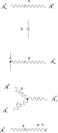
$$-2i/(k^{\rho}k_{\rho})$$ (12)

$$i/\!\!\not{\!p}$$ (13)

$$\frac{1}{2}ig\gamma_{-}t^{a}$$ (15)

$$\frac{1}{4}gf^{abc}\bigg{(}1/(k_{-}+i\epsilon{\textrm{s}gn}(k_{+}))$$ (16)

$$-1/(l_{-}+i\epsilon{\textrm{s}gn}(l_{+}))\bigg{)}(k^{\bot}+l^{\bot})^{2}$$ (17)

$$-ik^{\rho}/(k_{-}+i\epsilon{\textrm{s}gn}(k_{+}))$$ (18)

FIG. 1.: Feynman rules corresponding to the effective lagrangian (11).

Using these Feynman rules we can calculate the contribution of order $g$ to the ${\cal T}$-matrix element (${\cal S}=1+i{\cal T}$) corresponding to the diagram in Fig.2.

FIG. 2.: First order graph.

Demanding that the quark in the final state is on mass-shell we multiply the resulting expression by $2\pi\delta((p-k)^{2})$ and obtain the order $g$ contribution to the potential in the momentum space

$$A^{\rho}_{1}(k)=2gt^{a}(t^{a}_{1})\frac{k^{\rho}}{(k^{\bot})^{2}}\frac{1}{k_{-}-i\epsilon}2\pi\delta(k_{+})$$ (19)

Note that the product of the pole term in $k_{-}$ and $\delta(k_{+})$ appears as the limit of the Mandelstam-Leibbrandt prescription

$$\frac{1}{k_{-}+i\epsilon{\textrm{s}gn(k_{+})}}\delta\bigg{(}k_{+}(1-\frac{k_{-}}{p_{-}}))+\frac{k^{\perp 2}}{p_{-}}\bigg{)}\stackrel{{\scriptstyle{\textrm{f}or}\,\,p_{-}\to\infty\,}}{{\longrightarrow}}\frac{1}{k_{-}-i\epsilon}\delta(k_{+})\;$$ (20)

and it coincides with the regularization used in [3].

Expression (19) of course agrees with the corresponding contribution in [3] (see eq.(5)), so after performing a Fourier transformation

$$A^{\rho}_{1}(x)=\int\frac{d^{4}k}{(2\pi)^{4}}A^{\rho}_{1}(k)e^{ik(x-x_{1})}$$ (21)

and taking into account the interaction with the other lines shown in Fig.2 we reproduce the lowest order contribution to the potential (2), $A(x^{\perp},x_{+})|_{g}$:

$$A^{\rho}(x^{\perp},x_{+})|_{g\,eff.lagr.} = A^{\rho}(x^{\perp},x_{+})|_{g}=$$ (22)

$$= \frac{g}{2\pi}t^{a}\bigg{(}\frac{x^{\rho}-x_{1}^{\rho}}{|x^{\bot}-x_{1}^{\bot}|^{2}}\theta(x_{+}-x_{1+})(t^{a}_{1})+\frac{x^{\rho}-x_{2}^{\rho}}{|x^{\bot}-x_{2}^{\bot}|^{2}}\theta(x_{+}-x_{2+})(t^{a}_{2})\bigg{)}$$ (24)

$$-\frac{g}{2\pi}t^{a}\bigg{(}\frac{x^{\rho}-x_{1}^{\prime\rho}}{|x^{\bot}-x_{1}^{\prime\bot}|^{2}}\theta(x_{+}-x_{1+}^{\prime})(t^{a}_{1})+\frac{x^{\rho}-x_{2}^{\prime\rho}}{|x^{\bot}-x_{2}^{\prime\bot}|^{2}}\theta(x_{+}-x_{2+}^{\prime})(t^{a}_{2})\bigg{)}$$

Passing to the $g^{3}$-contribution let us note that contrary to the calculations done in [3], in the case of the effective lagrangian approach we have to calculate only one diagram shown in Fig.3.

FIG. 3.: Third order graph.

Its contribution to the ${\cal T}$-matrix multiplied by the corresponding factors and putting two lines in the final state on the mass-shell has the form

$$A^{\rho}_{3}(k,l) = -2ig^{3}t^{c}f^{bac}(t^{a}_{2})(t^{b}_{1})\frac{(k+l)^{\rho}}{(l^{\bot})^{2}(k^{\bot})^{2}}\frac{1}{(k+l)_{-}-i\epsilon}\bigg{(}\frac{1}{l_{-}-i\epsilon}-\frac{1}{k_{-}-i\epsilon}\bigg{)}(2\pi)^{2}\delta(k_{+})\delta(l_{+})$$ (25)

which has a similar but not identical structure as the final result given in [3] in eq.(10). By perfoming a double Fourier transform of expression (25)

$$A^{\rho}_{3}(x^{\perp},x_{-})=\int\frac{d^{4}k}{(2\pi)^{4}}\frac{d^{4}l}{(2\pi)^{4}}A^{\rho}_{3}(k,l)e^{il(x-x_{1})+ik(x-x_{2})}$$ (26)

and imposing the condition $x_{2+}>x_{1+}$ we see that only the term with the pole in $l_{-}$ gives a contribution for such ordering. Next, taking into account the remaining three contributions corresponding to the interaction of the gluons $k$ and $l$ with the lines $1\;2^{\prime}$, $1^{\prime}\;2$ and $1^{\prime}\;2^{\prime}$ we obtain the formula

$$A^{\rho}(x^{\perp},x_{-})|_{g^{3},eff.lagr.} = -\frac{g^{3}}{2(2\pi)^{2}}t^{a}f^{abc}(t^{b}_{1})(t^{c}_{2})\bigg{\{}\theta(x_{+}-x_{2+})\partial^{\rho}\bigg{[}\ln(\lambda|x^{\bot}-x_{2}^{\bot}|)\ln\frac{|x^{\bot}-x_{1}^{\bot}|}{|x^{\bot}-x^{\prime\bot}_{1}|}\bigg{]}$$ (28)

$$-\theta(x_{+}-x_{2+}^{\prime})\partial^{\rho}\bigg{[}\ln(\lambda|x^{\bot}-x_{2}^{\prime\bot}|)\ln\frac{|x^{\bot}-x_{1}^{\bot}|}{|x^{\bot}-x^{\prime\bot}_{1}|}\bigg{]}\bigg{\}}\;,$$

where the transverse gradient $\partial^{\rho}$ always acts on $x^{\perp}$. This result has to be compared with the $g^{3}$ contribution to the potential (2)

$$A^{\rho}(x^{\perp},x_{-})|_{g^{3}}\!\! = \!\!-\frac{g^{3}}{(2\pi)^{2}}t^{a}f^{abc}(t^{b}_{1})(t^{c}_{2})\ln\bigg{[}\frac{|x^{\bot}-x^{\bot}_{1}|}{|x^{\bot}-x^{\prime\bot}_{1}|}\bigg{]}\bigg{(}\frac{x^{\rho}-x_{2}^{\rho}}{|x^{\bot}-x_{2}^{\bot}|^{2}}\theta(x_{+}-x_{2+})$$ (30)

$$-\frac{x^{\rho}-x_{2}^{\prime\rho}}{|x^{\bot}-x_{2}^{\prime\bot}|^{2}}\theta(x_{+}-x_{2+}^{\prime})\bigg{)}.$$

We see that although both expressions (28) and (30) have a similar structure they differ substantially. The main difference apart of an overall coefficient lies in the fact that in the effective lagragian result the transverse gradient acts on both logarithms (which correspond to the propagators of the gluons with momenta $k$ and $l$), whereas in eq.(30) it acts only on one of them. Let us remark that the $\lambda$-dependence of eq. (28) drops out in the limit $x_{+}>>x_{2+},x^{\prime}_{2+}$.

In order to calculate the contribution of order $g^{5}$ averaged in the colour space of nucleon 1 in our effective theory we have to take into account only two diagrams shown in Fig. 4 (the analogous calculations of Feynman diagrams in the light-cone gauge involve 13 diagrams).

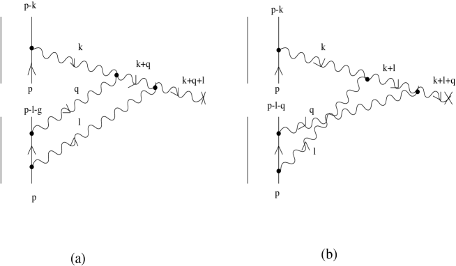
FIG. 4.: Fifth order graphs.

Calculating these diagrams we introduce two delta function factors which put two external lines in the final state on mass shell. Let us note that we are only interested in the classical contribution of the diagrams and therefore do not perform the loop-momentum integration but symmetrize the contributions with respect to $l$ and $q$ and use the following substitution

$$\frac{1}{l_{+}-i\epsilon}\delta(q_{+}+l_{+})\to\frac{1}{2}\left(\frac{1}{l_{+}-i\epsilon}+\frac{1}{q_{+}-i\epsilon}\right)\delta(q_{+}+l_{+})=i\pi\delta(l_{+})\delta(q_{+})\;.$$ (31)

The resulting expression is

$$<A^{\rho}_{5}(k,l,q)>_{1} = \!g^{5}t^{a}(t_{2}^{a})\frac{(k+l+q)^{\rho}}{(k^{\bot})^{2}(l^{\bot})^{2}(q^{\bot})^{2}}\frac{1}{(k+l+q)_{-}-i\epsilon}$$ (34)

$$\!\times\bigg{(}\frac{1}{(q_{-}-i\epsilon)(l_{-}-i\epsilon)}-\frac{1}{(q_{-}-i\epsilon)((k+q)_{-}-i\epsilon)}$$

$$\!-\frac{1}{(l_{-}-i\epsilon)((k+l)_{-}-i\epsilon)}\bigg{)}(2\pi)^{3}\delta(k_{+})\delta(l_{+})\delta(q_{+}).$$

We obtain the same answer if we put directly the fermionic line with momentum $p-l$ in the nucleon 1 on the mass-shell, i.e. if we take only the contribution of the delta function $i\pi\delta(l_{+})$ from the propagator into account.

By calculating now the triple Fourier transform of (34)

$\displaystyle<A^{\rho}_{5}(x^{\perp},x_{-})>_{1}=\int\frac{d^{4}k}{(2\pi)^{4}}\frac{d^{4}l}{(2\pi)^{4}}\frac{d^{4}q}{(2\pi)^{4}}<A^{\rho}_{5}(k,l,q)>_{1}e^{il(x-x_{1})+iq(x-x_{1})+ik(x-x_{2})}$

we obtain the expression

$$<A^{\rho}_{5}(x^{\perp},x_{-})>_{1}|_{eff.lagr.} = -\frac{g^{5}}{8(2\pi)^{3}}t^{a}(t_{2}^{a})\theta(x_{+}-x_{2+})\partial^{\rho}\bigg{(}\ln^{2}(\lambda|x^{\bot}-x_{1}^{\bot}|)\ln(\lambda|x^{\bot}-x_{2}^{\bot}|)\bigg{)}$$ (35)

which we can compare with the corresponding term obtained from the expansion of the classical potential (2) (see eq.(15) in [3]), being reproduced by the sum of the Feynman diagrams shown in Fig.5 in [3]

$$<A^{\rho}_{5}(x^{\perp},x_{-})>_{1}=-\frac{g^{5}}{4(2\pi)^{3}}t^{a}(t_{2}^{a})\theta(x_{+}-x_{2+})\ln^{2}(\lambda|x^{\bot}-x_{1}^{\bot}|)\frac{x^{\rho}-x_{2}^{\rho}}{|x^{\bot}-x_{2}^{\bot}|^{2}}.$$ (36)

Again we see that the main difference between both expressions (apart from a numerical factor of 2) is related to the fact that in (35) the transverse gradient acts on all propagators of the gluons with momenta $k$, $l$ and $q$ whereas in (36) it acts only on the propagator of the gluon with momentum $k$. Let us note that this feature of our result will persist in higher orders. The reason for this lies in the factorized form of the vertices in the longitudinal and transverse parts and in the fact that the transverse gradient is directly related to the coupling of the external current $J^{a}_{\rho}$. As a consequence it will always act on the whole expression of each diagram.

III Discussion

On the basis of our calculations we conclude that the potential obtained with the use of the effective lagrangian for high energy QCD differs from the classical potential of the ultrarelativistic nucleus on which the approach developed in [1] is based. This fact by itself should not be very surprising since as we already mentioned the classical and the effective potential correspond to different types of fields (our effective Gluon is a Reggeon). Taking into account that in both methods only classical contributions are calculated, it is suprising that the differences appear already in the lowest orders of perturbation theory. We expect these differences to persist in calculations for physical observables. As the effective lagrangian is derived from QCD with controlled, systematic and relatively mild assumptions we hope that our method will prove to be more successful in phenomenological applications. Presently our approach and that of Ref.[1] should simply be seen as alternatives. We want to stress also that our calculations along the line of [3] for the $g^{5}$-terms are very efficient because they build on the work invested in the derivation of the effective lagrangian.

Acknowledgements

We acknowledge stimulating discussions with Y. Kovchegov about the connection between both approaches.

L.Sz. would like to thank Lev Lipatov for discussion.

This work was supported by GSI and DFG. R.K. and L.Sz. would like to acknowledge the support from the German-Polish agreement on scientific and technological cooperation N-115-95.

REFERENCES

- [1] L. McLerran and R. Venugopalan, Phys. Rev. D 49, 2233 (1994), ibid D 49, 3352 (1994), ibid D 50, 2225 (1994)
- [2] Y.V. Kovchegov, Phys. Rev. D54, 5463 (1996)
- [3] Y.V. Kovchegov, Phys. Rev. D55, 5445 (1997)
- [4] L.N. Lipatov, Nucl. Phys. B 365, 614 (1991)
-
[5]
R. Kirschner, L.N. Lipatov and L. Szymanowski,
Nucl. Phys. B 425, 579 (1994)
R. Kirschner, L.N. Lipatov and L. Szymanowski, Phys. Rev. D 51, 838 (1995) - [6] L.N. Lipatov, Nucl. Phys. B 452, 369 (1995)
- [7] R. Kirschner and L. Szymanowski, Phys. Rev. D 58, 014004 (1998)
-
[8]
S. Mandelstam, Nucl. Phys. B 213, 140 (1983)
G. Leibbrandt, Phys. Rev. D 29, 1699 (1984)