SU-4240-693

$\eta^{\prime}\rightarrow\eta\pi\pi$ Decay as a Probe of
a Possible Lowest-Lying Scalar Nonet

Amir H. Fariborz and Joseph Schechter

Department of Physics, Syracuse University, Syracuse, NY 13244-1130, USA.

Abstract

We study the $\eta^{\prime}\rightarrow\eta\pi\pi$ decay within an effective chiral Lagrangian approach in which the lowest lying scalar meson candidates $\sigma(560)$ and $\kappa(900)$ together with the $f_{0}(980)$ and $a_{0}(980)$ are combined into a possible nonet. We show that there exists a unique choice of the free parameters of this model which, in addition to fitting the $\pi\pi$ and $\pi K$ scattering amplitudes, well describes the experimental measurements for the partial decay width of $\eta^{\prime}\rightarrow\eta\pi\pi$ and the energy dependence of this decay. As a by-product, we estimate the $a_{0}(980)$ width to be 70 MeV, in agreement with a new experimental analysis.

PACS number(s): 13.75.Lb, 11.15.Pg, 11.80.Et, 12.39.Fe

I Introduction

Understanding the status, in general, and the quark content, in particular, of the lowest lying scalar mesons is an issue of great current interest. In the cases of the $\sigma$ and the $\kappa$ mesons, even their existence has been the subject of many different investigations. One may consult refs.[1]-[16] for a variety of different recent works.

In the approach upon which this paper is based, a need for a $\sigma$ with a mass around 560 MeV was found in the analysis of $\pi\pi$ scattering [17, 18] and a need for a $\kappa$ with a mass around 900 MeV was required in order to describe the experimental data on the $\pi K$ scattering amplitude [19]. These investigations were carried out in an effective Lagrangian framework motivated by the $1/N_{c}$ approximation to QCD. In this approach, one incorporates the contribution of tree Feynman diagrams, computed from a chiral Lagrangian, including all possible intermediate states within the energy region of interest. Furthermore, crossing symmetry is automatic, while the unknown parameters characterizing the scalars are adjusted to satisfy the unitarity bounds. Approximate amplitudes satisfying both crossing and unitarity are then obtained. For the case of $\pi K$ scattering in the $I={1\over 2}$ channel the analysis of ref.[19] may be seen to be consistent with the experimental work of ref.[20]. The experimental analysis characterizes the data by an effective range approximation below 1 GeV; in the treatment of [19] it is resolved into the sum of a “current-algebra” piece, vector meson exchange pieces and scalar meson exchange pieces. In particular, the presence of a $\kappa$-meson is needed to ensure unitarity.

Motivated by the evidence for a $\sigma$ and a $\kappa$, and taking into account other experimentally well-established scalars – the $f_{0}(980)$ and the $a_{0}(980)$ – a possible classification of these scalars (all below 1 GeV) into a nonet,

$$N=\left[\begin{array}[]{c c c}N_{1}^{1}&a_{0}^{+}&\kappa^{+}\\ a_{0}^{-}&N_{2}^{2}&\kappa^{0}\\ \kappa^{-}&{\bar{\kappa}}^{0}&N_{3}^{3}\end{array}\right],$$ (1)

was studied in [21]. Since the properties of this scalar nonet are expected to be less standard than those of a conventional nonet (like the vectors), the mass piece of the effective Lagrangian is allowed to contain extra terms:

$${\cal L}_{mass}=-a{\rm Tr}(NN)-b{\rm Tr}(NN{\cal M})-c{\rm Tr}(N){\rm Tr}(N)-d{\rm Tr}(N){\rm Tr}(N{\cal M}),$$ (2)

where ${\cal M}$ is the usual quark mass spurion. Retaining just the $a$ and $b$ terms yields “ideal mixing” [22]. The physical particles $\sigma$ and $f_{0}$ which diagonalize the mass matrix are related to the basis states $N_{3}^{3}$ and $(N_{1}^{1}+N_{2}^{2})/{\sqrt{2}}$ by

$$\left(\begin{array}[]{c}\sigma\\ f_{0}\end{array}\right)=\left(\begin{array}[]{c c}{\rm cos}\theta_{s}&-{\rm sin}\theta_{s}\\ {\rm sin}\theta_{s}&{\rm cos}\theta_{s}\end{array}\right)\left(\begin{array}[]{c}N_{3}^{3}\\ \frac{N_{1}^{1}+N_{2}^{2}}{\sqrt{2}}\end{array}\right),$$ (3)

where $\theta_{s}$ is the scalar mixing angle. The coefficients $a,b,c,$ and $d$ are determined in terms of $m_{\sigma}$, $m_{f0}$, $m_{a0}$ and $m_{\kappa}$, and for a given input set of these masses there are two scalar mixing angles. Typical values of the input masses ($m_{\sigma}=550$ MeV, $m_{f0}=980$ MeV, $m_{a0}=983.5$ MeV and $m_{\kappa}=897$ MeV) yield the two possibilities:

$$\left(a\right)\quad {\theta}_{s} \>\approx\>-21^{\circ},$$ (4)

$$\left(b\right)\quad {\theta}_{s} \>\approx\>-89^{\circ}.$$ (5)

In order to determine which of these two possibilities is the correct one, it is necessary to study the pattern of scalar-pseudoscalar-pseudoscalar interactions, which are correlated with each other by the proposed nonet structure. In this picture, the general form of the SU(3) flavor invariant scalar-pseudoscalar-pseudoscalar interaction is:

$${\cal L}_{N\phi\phi} = A{\epsilon}^{abc}{\epsilon}_{def}N_{a}^{d}{\partial_{\mu}}{\phi}_{b}^{e}{\partial_{\mu}}{\phi}_{c}^{f}+B{\rm Tr}\left(N\right){\rm Tr}\left({\partial_{\mu}}\phi{\partial_{\mu}}\phi\right)+C{\rm Tr}\left(N{\partial_{\mu}}\phi\right){\rm Tr}\left({\partial_{\mu}}\phi\right)$$ (6)

$$+ D{\rm Tr}\left(N\right){\rm Tr}\left({\partial_{\mu}}\phi\right){\rm Tr}\left({\partial_{\mu}}\phi\right),$$ (7)

where $\phi_{a}^{b}\left(x\right)$ is the matrix of the pseudoscalar nonet fields, and $A,B,C,D$ are real parameters. Derivative coupling to the two pseudoscalars is used to ensure that Eq. (7) represents the leading term of a chiral invariant expression (see Appendix B of [21]). It is easy to see that all the coupling constants relevant for the study of $\pi\pi$ and $\pi K$ scattering depend only on the parameters $A$ and $B$. The analysis of [21] then shows that possibility (a) in (5) for the scalar mixing angle is selected as the correct one in the present scheme. The parameters $C$ and $D$ were left undetermined in the analysis of [21], as no scalar-pseudoscalar-pseudoscalar coupling involving an $\eta$ or $\eta^{\prime}$ was present in the $\pi\pi$ and $\pi K$ scattering discussed there.

In this work we explore the parameter space of $C$ and $D$ in detail by studying the $\eta^{\prime}\rightarrow\eta\pi\pi$ decay, for which there are relatively recent and precise experimental measurements. As we will see, the scalar couplings to $\eta$ and $\eta^{\prime}$ play a dominant role in the amplitude for this decay.

All the discussion in the present paper will use the same methods and parameters as in the previous $\pi\pi$ and $\pi K$ scattering papers [18, 19]. Thus, this work can be thought of as a check of that method as well as a test of the basic assumption that the low lying scalars are related to each other by belonging to a (broken) flavor SU(3) nonet. In the sense that the effective Lagrangian method makes no explicit reference to the quark structure of these scalars, the present work may be considered model independent. Note also that only the SU(3) flavor structure of the scalars is required to construct non-linear chiral Lagrangians describing these interactions [23].

“Microscopic” models of low lying scalars have been suggested in which they are variously $qq{\bar{q}}{\bar{q}}$ states in the MIT bag [24], meson-meson molecules [25] or unitarity corrections due to strong meson meson interactions [1, 12]. All these models involve four quarks and so may be related to each other. A “model-independent” effective Lagrangian might be an appropriate vehicle for summarizing the common feature of different microscopic models.

The process $\eta^{\prime}\rightarrow\eta\pi\pi$ has been studied by many authors in chiral symmetric frameworks since the early days of “Current-Algebra”. Treatments have used exclusively contact terms [26, 27, 28, 29] or contact terms plus scalar meson exchanges [30, 31, 32, 33]. Ordinarily in the chiral perturbation theory approach [34] all effects of resonance exchanges are assumed to be “integrated out” and summarized in the complete set of contact terms. However, in the case of the $\eta^{\prime}(958)$ decay, the masses of the intermediate $\sigma$, $f_{0}$ and $a_{0}$ resonances are either less than or comparable to 958 MeV. Thus, kinematical dependences due to the propagators could be important. The new features of the present treatment include the use of Eq.(2) to describe the scalar mesons and mixing angle, the use of Eq.(7) to describe the scalar coupling constants and a procedure uniform with the discussion of $\pi\pi$ and $\pi K$ scattering in [17, 18, 19]. Furthermore, comparison is being made with more recent data.

This paper is organized as follows. Section II gives our theoretical prediction of the $\eta^{\prime}\rightarrow\eta\pi\pi$ process as well as the experimental parameterization. The fit to the experiment, taking into account the experimental uncertainties, is treated in detail in Section III. Finally, Section IV continue a brief summary and discussion.

II $\eta^{\prime}\rightarrow\eta\pi\pi$ decay

Here, we will predict the amplitude for this process in the present model and display the experimental data to which it will be compared.

We assume exact iso-spin invariance which seems consistent with the present experimental accuracy. The four momenta of the particles are labeled according to the scheme $\eta^{\prime}(p)\rightarrow\eta(k)+\pi_{1}(q_{1})+\pi_{2}(q_{2})$, wherein ($\pi_{1},\pi_{2}$) can stand for either ($\pi^{+},\pi^{-}$) or ($\pi^{0},\pi^{0}$). The partial widths are related to the invariant matrix element $M(p\rightarrow k+q_{1}+q_{2})$ by

$$\Gamma(\eta^{\prime}\rightarrow\eta\pi^{+}\pi^{-})=2\Gamma(\eta^{\prime}\rightarrow\eta\pi^{0}\pi^{0})={1\over{2m_{\eta^{\prime}}}}\int|M|^{2}d\Phi,$$ (8)

where the phase space volume element $d\Phi$ is

$$d\Phi=(2\pi)^{4}\delta^{4}(p-k-q_{1}-q_{2}){{d{\bf k}}\over{2\omega(2\pi)^{3}}}{{d{\bf q_{1}}}\over{2\omega_{1}(2\pi)^{3}}}{{d{\bf q_{2}}}\over{2\omega_{2}(2\pi)^{3}}},$$ (9)

with $\omega=\sqrt{m_{\eta}^{2}+{\bf k}^{2}}$ and $\omega_{i}=\sqrt{m_{\pi}^{2}+{\bf q_{i}}^{2}}$. After performing the usual phase space integration we have

$$\Gamma_{\eta^{\prime}\rightarrow\eta\pi\pi}={1\over{64\pi^{3}m_{\eta}^{\prime}}}\int d{\omega_{1}}d{\omega_{2}}\left|M\right|^{2}.$$ (10)

The boundary of integration in the $\omega_{1}\omega_{2}$ plane for our choice of $m_{\pi}=137$ MeV, $m_{\eta}=547$ MeV and $m_{\eta^{\prime}}=958$ MeV [35] is shown in Fig.1.

FIG. 1.: The boundary of integration in Eq.(10).

In the treatment of $\pi\pi$ [17, 18] and $\pi K$ [19] scattering according to the present approach it was found that a reasonable approximation up to the 1 GeV energy range consisted of including i) the “current algebra” contact term ii) vector meson tree diagrams and iii) light scalar ($f_{0}(980),\sigma,\kappa$) meson tree diagrams. These were all calculated from a chiral Lagrangian with the minimum number of derivatives. For $\eta^{\prime}\rightarrow\eta\pi\pi$ there is a big simplification since G-parity conservation shows that no vector meson exchanges are possible at tree level. Similarly, the derivative part of the contact term vanishes.

The individual contributions shown in Fig.2 are then

$$M_{C.A.} = {{m_{\pi}^{2}}\over{F_{\pi}^{2}}}{\rm sin}2\theta_{p},$$ (11)

$$M_{\sigma} = -\sqrt{2}\gamma_{\sigma\eta\eta^{\prime}}\gamma_{\sigma\pi\pi}{{(p.k)(q_{1}.q_{2})}\over{m_{\sigma}^{2}+(p-k)^{2}-im_{\sigma}G^{\prime}_{\sigma}}},$$ (12)

$$M_{f_{0}} = -\sqrt{2}\gamma_{f\eta\eta^{\prime}}\gamma_{f\pi\pi}{{(p.k)(q_{1}.q_{2})}\over{m_{f_{0}}^{2}+(p-k)^{2}-im_{f0}G^{\prime}_{f0}}},$$ (13)

$$M_{a_{0}} = -\gamma_{a\pi\eta^{\prime}}\gamma_{a\pi\eta}\left[{{(p.q_{2})(k.q_{1})}\over{m_{a_{0}}^{2}+(p-q_{2})^{2}-im_{a0}G^{\prime}_{a0}}}+{{(p.q_{1})(k.q_{2})}\over{m_{a_{0}}^{2}+(p-q_{1})^{2}-im_{a0}G^{\prime}_{a0}}}\right].$$ (14)

FIG. 2.: Tree Feynman diagrams representing the contributions of (a) the current algebra, (b) the $\sigma$ and the $f_{0}(980)$, and (c) the $a_{0}(980)$ terms to the decay $\eta^{\prime}\rightarrow\eta\pi\pi$ in our model.

The total decay amplitude $M$ is the sum of these pieces. The current algebra contribution $M_{C.A.}$ is obtained from the “quark mass” term in the effective Lagrangian (proportional to ${\rm Tr}\left[(U+U^{\dagger}){\cal M}\right]$, where $U={\rm exp}\left[2i\phi/F_{\pi}\right]$). Definitions of the various scalar-pseudoscalar-pseudoscalar coupling constants which appear in the $\sigma,f_{0}(980)$ and $a_{0}(980)$ exchange diagrams are given in Appendix A. These involve the coefficients $A,B,C,D$ of Eq. (2);$A$ and $B$ were previously found from $\pi\pi$ and $\pi K$ scattering while $C$ and $D$ remain to be determined here. The scalar masses are taken as mentioned before Eq.(5). Even though there is no kinematical possibility for any of the intermediate scalars to be on the “mass shell” we include “total width” terms in the propagator denominators in order to agree with the previous work [17, 18, 19]. The $f_{0}$ and $a_{0}$ exchange terms will be essentially taken to be of Breit-Wigner form so $G^{\prime}_{f0}$ and $G^{\prime}_{a0}$ are related to the coupling constants. We take $G^{\prime}_{f0}=64.6$ MeV from [18] ([35] allows 40–100 MeV) and $G^{\prime}_{a0}=50-100$ MeV [35]. The exact value of $G^{\prime}_{a0}$ will be found from our analysis since it depends on the parameter $C$. Finally we take $G^{\prime}_{\sigma}=370$ MeV [35]; this is related to a pole position rather than a total Breit-Wigner width, a prescription which enables the construction of a $\pi\pi$ amplitude satisfying both the unitarity bounds and crossing symmetry.

The theoretical expressions in Eq. (8)-(14) will be compared with the experimental data on partial decay rates and energy dependence of $|M^{2}|$. The experimental results for the rates are listed [35] as:

$$\Gamma^{exp}_{\eta^{\prime}\rightarrow\eta\pi^{+}\pi^{-}} = 0.089\pm 0.010\hskip 4.26773pt{\rm MeV}$$ (15)

$$2\Gamma^{exp}_{\eta^{\prime}\rightarrow\eta\pi^{0}\pi^{0}} = 0.084\pm 0.012\hskip 4.26773pt{\rm MeV}$$ (16)

in agreement with iso-spin invariance. Since we are working in the iso-spin invariant limit we will average these to obtain:

$$\Gamma^{exp}_{\eta^{\prime}\rightarrow\eta\pi\pi}=0.0872\pm 0.008\hskip 4.26773pt{\rm MeV},$$ (17)

with which the theoretical results will be compared.

For describing the energy dependence, experimentalists use the Dalitz-like variables[36]:

$$x = {\sqrt{3}\over Q}(\omega_{1}-\omega_{2})$$ (18)

$$y = -{{2+m_{\eta}/m_{\pi}}\over Q}(\omega_{1}+\omega_{2})-1+{{2+m_{\eta}/m_{\pi}}\over Q}(m_{\eta^{\prime}}-m_{\eta})$$ (19)

with $Q=m_{\eta^{\prime}}-m_{\eta}-2m_{\pi}$. As $\omega_{1}$ and $\omega_{2}$ vary over the physical region in Fig.1, $x$ ranges from about -1.4 to 1.4 and $y$ ranges from -1 to about 1.2. One may expand the matrix element, up to an irrelevant overall phase, as

$$M={\cal A}^{1/2}\left[1+\beta_{1}y+\beta_{2}y^{2}+\gamma_{2}x^{2}\right]+\cdots$$ (20)

where ${\cal A}$ is real while $\beta_{1}$, $\beta_{2}$ and $\gamma_{2}$ are complex. The expansion begins with $x^{2}$ since $M$ (see for example Eq.(14)) must be invariant on the interchange $q_{1}\leftrightarrow q_{2}$, which implies $x\leftrightarrow-x$. It is found [36] that this form yields an $M^{2}$ which fits the experimental data when the $yx^{2}$, $y^{3}$, $x^{4}$ and $y^{2}x^{2}$ terms are negligible:

$$|M|^{2}={\cal A}\left[\left|1+\alpha y\right|^{2}+{\tilde{c}}x^{2}\right]+\cdots$$ (21)

Here $\alpha$ is complex and ${\tilde{c}}$ is real. For the decay $\eta^{\prime}\rightarrow\eta\pi^{0}\pi^{0}$, the experimental values are [36]

$${\rm Re}\hskip 4.26773pt\alpha = -0.058\pm 0.013$$ (22)

$${\rm Im}\hskip 4.26773pt\alpha = 0.00\pm 0.13$$ (23)

$${\tilde{c}} = 0.00\pm 0.03,$$ (24)

and for the decay $\eta^{\prime}\rightarrow\eta\pi^{+}\pi^{-}$

$${\rm Re}\hskip 4.26773pt\alpha=-0.08\pm 0.03.$$ (25)

As explained before, we compare our results with the average of the experimental data for charged and neutral pions. This means we should match our results to

$${\rm Re}\hskip 4.26773pt\alpha = -0.062\pm 0.012$$ (26)

$${\rm Im}\hskip 4.26773pt\alpha = 0.00\pm 0.13$$ (27)

$${\tilde{c}} = 0.00\pm 0.03.$$ (28)

The parameter ${\cal A}$ in Eq.(21) is determined using Eq. (17).

Altogether, the experimental data are fit with the four real quantities ${\cal A}$, Re $\alpha$, Im $\alpha$ and ${\tilde{c}}$. On the other hand the theoretical expression in Eq.(14) is completely fixed if we specify just the two real constants $C$ and $D$ in Eq. (2), since everything else is already specified. Clearly there is no a priori guarantee that we can fit the data using the present model. Furthermore, it is necessary for the expansion of Eq.(14) to also yield negligible higher order terms in Eq.(21). We will see in the next section that there in fact exists a unique choice of $C$ and $D$ which can fit the experimental data.

III Fit to Experiment

Our job is to find the parameters $C$ and $D$ so that $|M|^{2}$ computed from Eq.(14) agree with the experimental form given in Eqs. (21) , (17) and (28) up to the stated uncertainties.

As a preliminary we note that restrictions on the allowed values of $C$ may be obtained from experimental information on $a_{0}(980)\rightarrow\pi\eta$ decay. This partial width is given by

$$\Gamma(a_{0}\rightarrow\pi\eta)={\gamma_{a\pi\eta}^{2}q\over{32\pi m_{a0}^{2}}}\left(m_{a0}^{2}-m_{\pi}^{2}-m_{\eta}^{2}\right)$$ (29)

where $q$ is the center of mass momentum of the final state mesons. Now Eq.(A23) of Appendix A shows that $\gamma_{a\pi\eta}$ depends on the known values of $A$ and $\theta_{p}$ as well as the unknown value of $C$. The Review of Particle Properties [35] lists the total $a_{0}$ width as 50–100 MeV and the $\pi\eta$ mode as “dominant”. It was estimated in the present model (section IV of [21]) that $\Gamma(a_{0}\rightarrow K{\bar{K}})$ is only about 5 MeV so we expect $G^{\prime}_{a0}\approx\Gamma(a_{0}\rightarrow\pi\eta)$ + 5 MeV. We conservatively expect $\Gamma(a_{0}\rightarrow\pi\eta)$ to lie in the range 25–100 MeV. This restricts $C$ to the two intervals [-21, -13] GeV^-1 and [2, 10.5] GeV^-1.

For initial orientation we shall neglect the imaginary terms in the denominators of Eq.(14). We start by numerically scanning the above two intervals of $C$ and searching for the acceptable regions in the $CD$ plane that are consistent with the averaged experimental partial decay width (17). The result of this search is shown in Fig. 3 which also shows the analogous intervals when the imaginary terms in Eq.(14) are retained. For $C$ in the interval [-13, -21] GeV^-1 there is a small acceptable region, whereas for $C$ in [2, 10.5] GeV^-1 there are two acceptable regions in the form of strips along the $C$ axis. In both intervals the thickness of these regions is related to the error in the averaged experimental partial decay width in (17), and therefore, is the main source of our error estimation in the final evaluation of $C$ and $D$. It turns out that it is a reasonable approximation to neglect the additional uncertainty associated with the stated error in Re $\alpha$. In order to further restrict the acceptable values of $C$ and $D$, we compare our predicted energy dependence, ${\left|M(x,y)\right|^{2}}/{\left|M(0,0)\right|^{2}}$, with the experimental result (21) and (28) taking Im $\alpha\equiv 0$ for now and ${\tilde{c}}$ as a fitting parameter. We find that only the region around $C=7$ with negative $D$ has the required property and therefore we are left with the lower strip in Fig.3. In Fig.4 this region is enlarged; also shown is the line representing a set of “least squared” minima on which $\alpha$ is fixed. For a given $C$, the corresponding minimum is obtained by varying $D$ and ${\tilde{c}}$. The intersection of this line with the previous region yields the desired $C$ and $D$ estimates. Note that the fit improves in the direction of increasing $C$. The values of $C$ and $D$ are displayed in the first column of Table I.

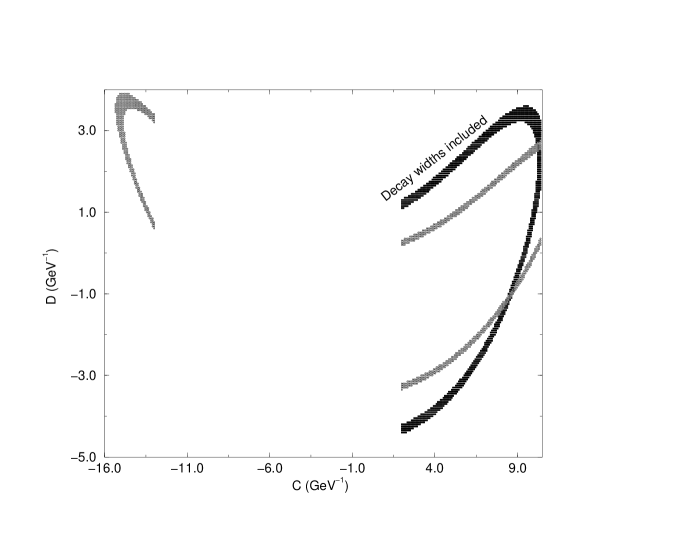
FIG. 3.: Regions consistent with the partial decay width of $\eta^{\prime}\rightarrow\eta\pi\pi$ and $a_{0}(980)\rightarrow\pi\eta$. The semi-closed region on the right is obtained by inclusion of the decay widths in the propagators of the intermediate scalars. $G^{\prime}_{\sigma}=370$ MeV, $G^{\prime}_{f0}=64.4$ MeV and $G^{\prime}_{a0}=100$ MeV. The other regions correspond to neglecting the decay widths.

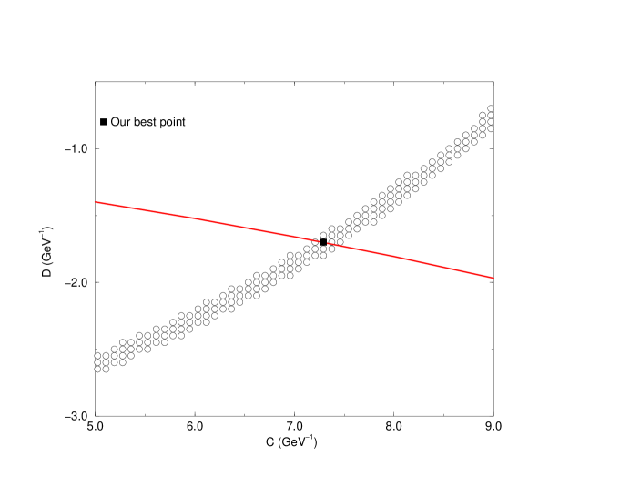
FIG. 4.: Extracting $C$ and $D$ from two different experimental measurements on $\eta^{\prime}$ decay. Circles represent the region consistent with the partial decay width of $\eta^{\prime}$, and the solid line represents the least squared fits of the normalized magnitude squared of the decay matrix element to the form $(1+\alpha y)^{2}+{\tilde{c}}x^{2}$ with $\alpha=-0.0615$.

$\begin{array}[]{|c||c|c|c|}\hline\cr A({\rm GeV}^{-1})&2.51&2.51&2.87\\ \hline\cr B({\rm GeV}^{-1})&-1.95&-1.95&-2.34\\ \hline\cr C({\rm GeV}^{-1})&7.29\pm 0.08&7.16\pm 0.13&7.25\pm 0.10\\ \hline\cr D({\rm GeV}^{-1})&-1.70\pm 0.08&-2.26\pm 0.13&-2.09\pm 0.10\\ \hline\cr{\rm Im}\hskip 4.26773pt\alpha&0&-0.12\pm 0.27&-0.16\pm 0.20\\ \hline\cr{\tilde{c}}&-0.004\pm 0.031&-0.014\pm 0.033&-0.013\pm 0.033\\ \hline\cr\Sigma&1.49&0.0032&0.0045\\ \hline\cr\end{array}$

TABLE I.: Extracted parameters from a fit of the normalized magnitude of the $\eta^{\prime}$ decay matrix element to the form $(1+\alpha y)^{2}+cx^{2}$, with Re $\alpha=-0.0615$. In the first and second columns $m_{\kappa}=897$ MeV while in the last column $m_{\kappa}=875$ MeV. The imaginary terms in the propagator denominators were not included for column 1. $\Sigma$ is the least square deviation with 1701 data points measuring the goodness of fit.

Now let us include the imaginary terms in the denominators of Eq.(14). In our computation we choose $G^{\prime}_{\sigma}=370$ MeV and $G^{\prime}_{f0}=64.6$ MeV as were obtained in [18], and the two extreme possibilities $G^{\prime}_{a0}=50,100$ MeV. We rescan the $CD$ plane for regions that are consistent with the partial decay width (17). The result is shown in Fig.3 and is also compared with the previous case where no widths were included. This figure shows that in the new case, there is no available region for $C$ in the interval [-21, -13] GeV^-1. For $C$ in the interval [2, 10.5] GeV^-1, we have shown in Fig.5 that the main effect of the inclusion of the decay widths is driven by the $\sigma$ width. In Fig.6, we have shown that the uncertainty in $G^{\prime}_{a0}$ does not make a substantial difference, in particular in the physical region where $C\approx 7$.

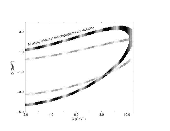
FIG. 5.: The effect of including the widths in the propagators is dominated by $G^{\prime}_{\sigma}$. In the two parallel regions in the middle, $G^{\prime}_{\sigma}$ is removed from its propagator.

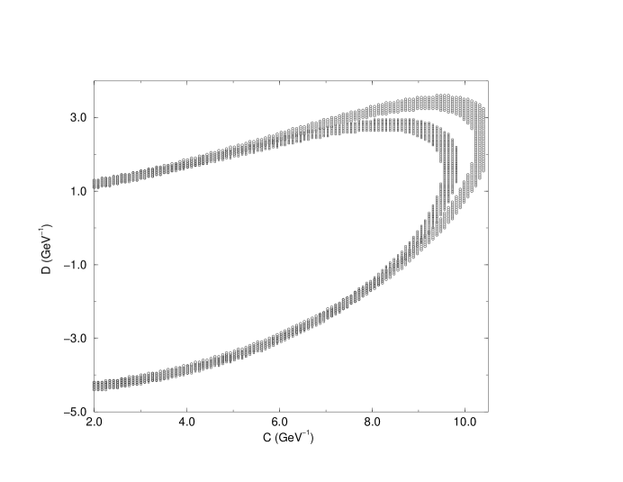
FIG. 6.: The available region consistent with the partial decay width of $\eta^{\prime}\rightarrow\eta\pi\pi$ is not sensitive to $G^{\prime}_{a0}$ in the physical region of $C\approx 7$. The outer/inner regions are obtained with $G^{\prime}_{a0}$=100/50 MeV.

We proceed as before, further restricting the available regions in the $CD$ plane by fitting the normalized magnitude of the decay matrix element $M$ to the form (21) with complex $\alpha$. We set ${\rm Re}\alpha=-0.0615$ and fit for ${\rm Im}\alpha$ and ${\tilde{c}}$ in this region. We find that the acceptable region in this case is very close to the previous region in Fig.4. The result is shown in Fig.7. The two lines correspond to two values of $G^{\prime}_{a0}$, and their intersections with the acceptable region for $\eta^{\prime}$ partial decay width provide our best points in this plane. We however notice that $C$ and $D$ for the value of $G^{\prime}_{a0}=50$ MeV correspond to a value of $\Gamma(a_{0}(980)\rightarrow\pi\eta)\approx 64$ MeV which is greater than the total decay width itself and cannot be correct. This consistency check within our computation further restricts the experimentally unknown value of $G^{\prime}_{a0}$. On the other hand, the intersection of the line corresponding to $G^{\prime}_{a0}=100$ MeV with the acceptable region of $\eta^{\prime}$ partial decay width gives $\Gamma_{a0(980)\rightarrow\pi\eta}\approx 65$ MeV. Therefore we conclude that our computation provides a stable estimate of the partial decay width of $a0(980)\rightarrow\pi\eta$ to be approximately 65 MeV.

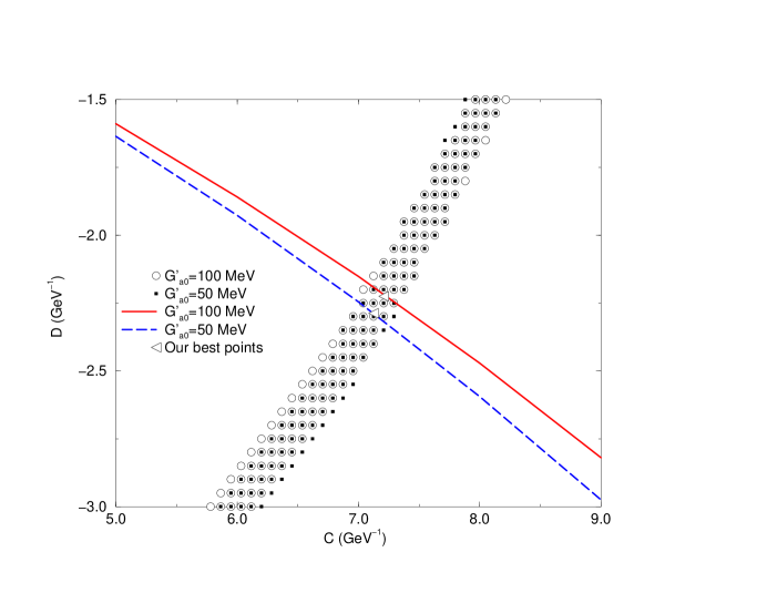
FIG. 7.: Extracting $C$ and $D$ from two different experimental measurements on $\eta^{\prime}$ decay. Circles represent the region which is consistent with the partial decay width of $\eta^{\prime}$, and lines represent the least squared fits of the normalized magnitude of decay matrix element to the form $\left|1+\alpha y\right|^{2}+{\tilde{c}}x^{2}$ with Re $\alpha=-0.0615$, $G^{\prime}_{\sigma}=370$ MeV and $G^{\prime}_{f0}=64.6$ MeV.

The only other hadronic $a_{0}$ decay mode which has been observed [35] is $K{\bar{K}}$; using $\Gamma(a_{0}\rightarrow K{\bar{K}})\approx 5$ MeV [21] we get an estimate $\Gamma_{tot}(a_{0})\approx 70$ MeV. The extracted values of $C$ and $D$ and other fitting parameters are listed in the second column of Table I. Note that the goodness of fit improves appreciably when we allow for non-zero widths.

It is perhaps interesting to display the $x$ and $y$ dependences of our normalized matrix element squared $|{\hat{M}}|^{2}={{|M(x,y)|^{2}}/{|M(0,0)|^{2}}}$. In Fig.8 we show the projections of this two dimensional surface onto the $y-|{\hat{M}}|^{2}$ and $x-|{\hat{M}}|^{2}$ planes. It is clear from the $y-|{\hat{M}}|^{2}$ projection that $|{\hat{M}}|^{2}$ has very little dependence on $x$.

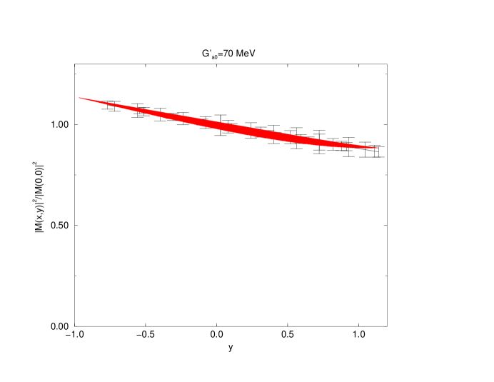
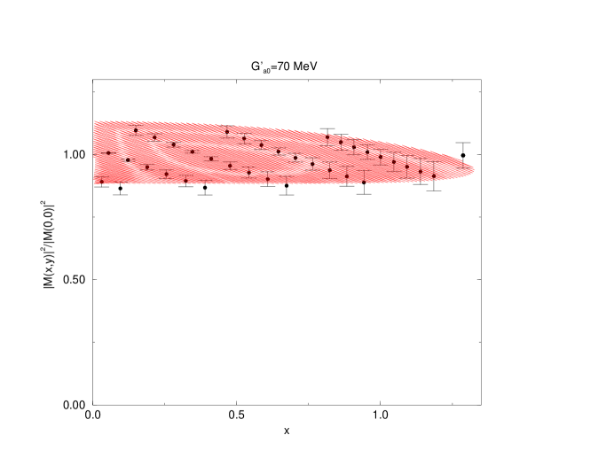
FIG. 8.: Projections of $|{\hat{M}}|^{2}=|M(x,y)|^{2}/|M(0,0)|^{2}$ onto the $y-|{\hat{M}}^{2}|$ and $x-|{\hat{M}}^{2}|$ planes. Parameters as in the second column of Table I.

The value of the scalar mixing angle $\theta_{s}\approx-21^{\circ}$ affects the entire calculation by its presence in the formulas[(A16)-(A36)] relating the scalar coupling constants to the parameters $A$, $B$, $C$ and $D$. Now $\theta_{s}$ is itself determined by diagonalizing the isoscalar mass squared matrix obtained from Eq.(2). In this way, $\theta_{s}$ depends on the input value of $m_{\kappa}$. The value $\theta_{s}\approx-20.33^{o}$ corresponds to $m_{\kappa}=897$ MeV but it was shown in [21] that a range $865MeV<m_{\kappa}<900$ MeV gave an acceptable description of $\pi K$ scattering. Furthermore, reducing $m_{\kappa}$ to 800 MeV results in the “ideal” case where $\theta_{s}=0^{o}$. In order to judge the sensitivity of our results to changing $m_{\kappa}$ we repeat the present computation for two lower values $m_{\kappa}=875$ and 800 MeV. As before we scan the $CD$ plane for the acceptable regions consistent with the $\eta^{\prime}\rightarrow\eta\pi\pi$ decay width (17). We display the results in Fig.9 which shows that the main effect of lowering $m_{\kappa}$ is in the $D>-1$ GeV^-1 region , far from the physical region in which we extract $C$ and $D$. We see in the same figure that for $C\approx 4\rightarrow 8$ the effect of changing $m_{\kappa}$ is negligible. In Fig.10 we have displayed these regions together with the corresponding least squared fits of the normalized magnitude of the decay matrix element of the form (21). As we see clearly in this figure, the value of $C$ extracted at the intersection of the lines with the strips changes by a very small amount as we go from $m_{\kappa}$=897 to 875 MeV. On the other hand, when we go to the lower value of $m_{\kappa}$=800 MeV, the the goodness of fit decreases and in particular for $C<7$GeV^-1 we get unacceptable fits. Furthermore, for $m_{\kappa}=800$ MeV we get the partial decay width of $a_{0}(980)\rightarrow\pi\eta$ to be 124 MeV which is greater than the total decay width and is inconsistent. This agrees with the observation in [21] that the values $m_{\kappa}<875$ MeV are not favored. For the value $m_{\kappa}=$875 MeV the details of the fit are given in the third column of Table I.

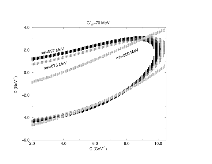
FIG. 9.: The effect of $m_{\kappa}$ on the acceptable regions consistent with the $\eta^{\prime}$ partial decay width. $G^{\prime}_{\sigma}=370$ MeV and $G^{\prime}_{f0}=64.6$ MeV.

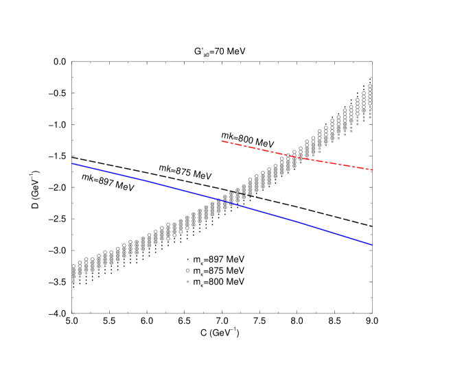
FIG. 10.: Sensitivity of our computation to $m_{\kappa}$. Strips represent regions consistent with the partial decay width of $\eta^{\prime}$, and lines represents the best least squared fits of the normalized magnitudes of decay matrix element to the form $\left|1+\alpha y\right|^{2}+cx^{2}$ with ${\rm Re}\alpha=-0.0615$. $G^{\prime}_{\sigma}=370$ MeV and $G^{\prime}_{f0}=64.6$ MeV.

IV Summary and Discussion

In this work, we studied in detail the $\eta^{\prime}\rightarrow\eta 2\pi$ decay mode within the framework of a model in which the scalar meson candidates $\sigma(560)$ (discussed in [18]) and $\kappa(900)$ (discussed in [19]) are combined into a nonet together with the $f_{0}(980)$ and the $a_{0}(980)$. The scalar mixing angle was calculated [21] in terms of these masses using Eq.(2) and the various scalar-pseudoscalar-pseudoscalar coupling constants were calculated in terms of the parameters $A$, $B$, $C$ and $D$ in Eq.(7). In the analysis of ref.[21] the parameters $A$, $B$ and $\theta_{s}$ were found, but parameters $C$ and $D$ were left undetermined. As $\eta^{\prime}$ decay probes these parameters, we have numerically searched this parameter space and found a unique $C$ and $D$ which describes the experimental measurements on the partial decay width of the $\eta^{\prime}\rightarrow\eta\pi\pi$ as well as its energy dependence.

Taking into account both the uncertainties in the scalar mixing angle $\theta_{s}$ (as reflected in the value of $m_{\kappa}$) and in the $\eta^{\prime}\rightarrow\eta\pi\pi$ decay width we get for the scalar coupling parameters

$$A = 2.51\rightarrow 2.87\hskip 4.26773pt{\rm GeV}^{-1}$$ (30)

$$B = -1.95\rightarrow-2.34\hskip 4.26773pt{\rm GeV}^{-1}$$ (31)

$$C = 7.03\rightarrow 7.39\hskip 4.26773pt{\rm GeV}^{-1}$$ (32)

$$D = -2.39\rightarrow-1.95\hskip 4.26773pt{\rm GeV}^{-1}$$ (33)

These numbers are based on combining the second and third columns of Table I. The coupling constants relevant here are listed in Table II.

As a by-product of the present calculation we obtain an estimate of the $a_{0}(980)$ width

$$\Gamma\left(a_{0}(980)\right)\approx 70{\rm MeV}$$ (34)

as discussed in Section III. After this work was completed we found a very new experimental analysis [37] of the $\pi^{-}p\rightarrow\eta\pi^{+}\pi^{-}$ and $\pi^{-}p\rightarrow\eta\pi^{0}n$ reactions which yields the same result we have obtained from analysis of the $\eta^{\prime}\rightarrow\eta\pi\pi$ decay.

It seems useful to “dissect” our model in order to get a qualitative understanding of the $\eta^{\prime}\rightarrow\eta\pi\pi$ process. Thus we have plotted, in Fig.11, the real and imaginary parts of the individual contributions of the terms in Eq.(14) to the total decay matrix element. These figures again represent projections of the Re $M(x,y)$ and Im $M(x,y)$ surfaces onto the Re $M-y$ and Im $M-y$ planes; the small $x$ dependences are thus visible as thickening of the curves. First, we observe that the “current-algebra” part of the amplitude, which corresponds to the use of the minimal non-linear chiral Lagrangian of pseudoscalar fields, is an order of magnitude too small to explain the experimental result by itself. On the other hand, the $a_{0}(980)$ exchange contribution is clearly the main one for explaining the dominant real part of the amplitude. Nevertheless the other contributions are not negligible. For example the cross term 2 [Re $M(\sigma)$] [Re $M(a_{0})$] is of the same order as [Re $M(a_{0})$]². Furthermore the $\sigma$ meson exchange is seen to give the largest contribution to Im $M$ for most of the kinematical range.

FIG. 11.: Projections onto the Re $(M_{i})-y$ and Im $(M_{i})-y$ planes of the individual scalar contributions  to the decay matrix element corresponding to the result given in the second column of Table I.

Note that we have used just the two input numbers, $C$ and $D$ (over and above the ones previously found) to satisfactorily fit the rate and energy distribution of $\eta^{\prime}\rightarrow\eta\pi\pi$. Thus in the same framework, with the same parameters, we are explaining $\pi\pi$ [18] and $\pi K$ [19] scattering up to the 1 GeV range as well as $\eta^{\prime}\rightarrow\eta\pi\pi$. Our results may then be regarded as support for the correctness of both the large $N_{c}$ approximation motivated approach to low energy dynamics being employed as well as the effective Lagrangian model [21] for the low lying scalar nonet outlined in the Introduction. Of course, the “microscopic” structure of low lying scalars is an interesting puzzle of present day particle physics which seems to require a great deal of further experimental and theoretical work for its clarification. For example, the study of radiative decays of the $\phi(1020)$ is expected [38] to yield useful information. As discussed in more detail in [21], the value of the mixing angle $\theta_{s}$, about $-21^{\circ}$ and the mass spectrum used here are what one would expect with a somewhat distorted form of the $qq{\bar{q}}{\bar{q}}$ model [24]. A priori, however, our effective Lagrangian approach can accommodate any microscopic model which yields a flavor nonet.

A

Here we give, for convenience, the explicit form of the scalar-pseudoscalar-pseudoscalar interaction [21]. Using isotopic spin invariance, the trilinear $N\phi\phi$ interaction from Eq. (7) must have the form:

$$-{\cal L}_{N\phi\phi} = \frac{\gamma_{\kappa K\pi}}{\sqrt{2}}\left(\partial_{\mu}{\bar{K}}\mbox{\boldmath${\tau}$}\cdot\partial_{\mu}{\mbox{\boldmath${\pi}$}}\kappa+h.c.\right)+\frac{\gamma_{\sigma\pi\pi}}{\sqrt{2}}\sigma\partial_{\mu}\mbox{\boldmath${\pi}$}\cdot\partial_{\mu}{\mbox{\boldmath${\pi}$}}$$ (A1)

$$+ \frac{\gamma_{\sigma KK}}{\sqrt{2}}\sigma\partial_{\mu}{\bar{K}}\partial_{\mu}{K}+\frac{\gamma_{f_{0}\pi\pi}}{\sqrt{2}}f_{0}\partial_{\mu}\mbox{\boldmath${\pi}$}\cdot\partial_{\mu}\mbox{\boldmath${\pi}$}+\frac{\gamma_{f_{0}KK}}{\sqrt{2}}f_{0}\partial_{\mu}{\bar{K}}\partial_{\mu}{K}$$ (A2)

$$+ \frac{\gamma_{a_{0}KK}}{\sqrt{2}}\partial_{\mu}{\bar{K}}\mbox{\boldmath${\tau}$}\cdot{\bf a_{0}}\partial_{\mu}{K}+\gamma_{\kappa{K}\eta}\left({\bar{\kappa}}\partial_{\mu}K\partial_{\mu}{\eta}+h.c.\right)+\gamma_{\kappa{K}\eta^{\prime}}\left({\bar{\kappa}}\partial_{\mu}K\partial_{\mu}{\eta^{\prime}}+h.c.\right)$$ (A3)

$$+ \gamma_{a_{0}\pi\eta}{\bf a_{0}}\cdot\partial_{\mu}\mbox{\boldmath${\pi}$}\partial_{\mu}\eta+\gamma_{a_{0}\pi\eta^{\prime}}{\bf a_{0}}\cdot\partial_{\mu}\mbox{\boldmath${\pi}$}\partial_{\mu}\eta^{\prime}$$ (A4)

$$+ \gamma_{\sigma\eta\eta}\sigma\partial_{\mu}\eta\partial_{\mu}\eta+\gamma_{\sigma\eta\eta^{\prime}}\sigma\partial_{\mu}\eta\partial_{\mu}\eta^{\prime}+\gamma_{\sigma\eta^{\prime}\eta^{\prime}}\sigma\partial_{\mu}\eta^{\prime}\partial_{\mu}\eta^{\prime}$$ (A5)

$$+ \gamma_{f_{0}\eta\eta}f_{0}\partial_{\mu}\eta\partial_{\mu}\eta+\gamma_{f_{0}\eta\eta^{\prime}}f_{0}\partial_{\mu}\eta\partial_{\mu}\eta^{\prime}+\gamma_{f_{0}\eta^{\prime}\eta^{\prime}}f_{0}\partial_{\mu}\eta^{\prime}\partial_{\mu}\eta^{\prime},$$ (A6)

where the $\gamma$’s are the coupling constants. The fields which appear in this expression are the isomultiplets:

$$K=\left(\begin{array}[]{c}K^{+}\\ K^{0}\end{array}\right),\quad{\bar{K}}=\left(\begin{array}[]{cc}K^{-}&{\bar{K}^{0}}\end{array}\right) \quad\kappa=\left(\begin{array}[]{c}\kappa^{+}\\ \kappa^{0}\end{array}\right),\quad{\bar{\kappa}}=\left(\begin{array}[]{cc}{\kappa}^{-}&{\bar{\kappa}^{0}}\end{array}\right),$$ , (A13)

$$\pi^{\pm}=\frac{1}{\sqrt{2}}\left(\pi_{1}\mp i\pi_{2}\right) \quad\pi^{0}=\pi_{3},$$ , (A14)

$$a_{0}^{\pm}=\frac{1}{\sqrt{2}}\left(a_{01}\mp ia_{02}\right) \quad a_{0}^{0}=a_{03},$$ , (A15)

in addition to the isosinglets $\sigma$, $f_{0}$, $\eta$ and $\eta^{\prime}$. The $\gamma$’s are related to parameters $A$, $B$, $C$, $D$ of Eq. (7) by

$$\gamma_{\kappa K\pi} = \gamma_{a_{0}KK}=-2A$$ (A16)

$$\gamma_{\sigma\pi\pi} = 2B{\rm sin}\theta_{s}-\sqrt{2}(B-A){\rm cos}\theta_{s}$$ (A17)

$$\gamma_{\sigma K{K}} = 2(2B-A){\rm sin}\theta_{s}-2\sqrt{2}B{\rm cos}\theta_{s}$$ (A18)

$$\gamma_{f_{0}\pi\pi} = \sqrt{2}(A-B){\rm sin}\theta_{s}-2B{\rm cos}\theta_{s}$$ (A19)

$$\gamma_{f_{0}K{K}} = 2(A-2B){\rm cos}\theta_{s}-2\sqrt{2}B{\rm sin}\theta_{s}$$ (A20)

$$\gamma_{\kappa{K}\eta} = C{\rm sin}\theta_{p}-\sqrt{2}(C-A){\rm cos}\theta_{p}$$ (A21)

$$\gamma_{\kappa{K}\eta^{\prime}} = \sqrt{2}(A-C){\rm sin}\theta_{p}-C{\rm cos}\theta_{p}$$ (A22)

$$\gamma_{a_{0}\pi\eta} = (C-2A){\rm sin}\theta_{p}-\sqrt{2}C{\rm cos}\theta_{p}$$ (A23)

$$\gamma_{a_{0}\pi\eta^{\prime}} = (2A-C){\rm cos}\theta_{p}-\sqrt{2}C{\rm sin}\theta_{p}$$ (A24)

$$\gamma_{\sigma\eta\eta} = \left[\sqrt{2}(B+D)-{1\over 2}(C+2A+4D){\rm sin}2\theta_{p}+\sqrt{2}(C+D){\rm cos}^{2}\theta_{p}\right]{\rm sin}\theta_{s}$$ (A26)

$$-\left[(B+D)-{1\over\sqrt{2}}(C+2D){\rm sin}2\theta_{p}+(A+D){\rm cos}^{2}\theta_{p}+C{\rm sin}^{2}\theta_{p}\right]{\rm cos}\theta_{s}$$

$$\gamma_{\sigma\eta^{\prime}\eta^{\prime}} = \left[\sqrt{2}(B+D)+{1\over 2}(C+2A+4D){\rm sin}2\theta_{p}+\sqrt{2}(C+D){\rm sin}^{2}\theta_{p}\right]{\rm sin}\theta_{s}$$ (A28)

$$-\left[(B+D)+{1\over\sqrt{2}}(C+2D){\rm sin}2\theta_{p}+(A+D){\rm sin}^{2}\theta_{p}+C{\rm cos}^{2}\theta_{p}\right]{\rm cos}\theta_{s}$$

$$\gamma_{\sigma\eta\eta^{\prime}} = \left[\sqrt{2}(C+D){\rm sin}2\theta_{p}+(C+2A+4D){\rm cos}2\theta_{p}\right]{\rm sin}\theta_{s}$$ (A30)

$$-\left[\sqrt{2}(C+2D){\rm cos}2\theta_{p}+(A-C+D){\rm sin}2\theta_{p}\right]{\rm cos}\theta_{s}$$

$$\gamma_{f_{0}\eta\eta} = \left[-\sqrt{2}(B+D)+{1\over 2}(C+2A+4D){\rm sin}2\theta_{p}-\sqrt{2}(C+D){\rm cos}^{2}\theta_{p}\right]{\rm cos}\theta_{s}$$ (A32)

$$-\left[(B+D)-{1\over\sqrt{2}}(C+2D){\rm sin}2\theta_{p}+(A+D){\rm cos}^{2}\theta_{p}+C{\rm sin}^{2}\theta_{p}\right]{\rm sin}\theta_{s}$$

$$\gamma_{f_{0}\eta^{\prime}\eta^{\prime}} = -\left[\sqrt{2}(B+D)+{1\over 2}(C+2A+4D){\rm sin}2\theta_{p}+\sqrt{2}(C+D){\rm sin}^{2}\theta_{p}\right]{\rm cos}\theta_{s}$$ (A34)

$$-\left[(B+D)+{1\over\sqrt{2}}(C+2D){\rm sin}2\theta_{p}+(A+D){\rm sin}^{2}\theta_{p}+C{\rm cos}^{2}\theta_{p}\right]{\rm sin}\theta_{s}$$

$$\gamma_{f_{0}\eta\eta^{\prime}} = -\left[\sqrt{2}(C+D){\rm sin}2\theta_{p}+(C+2A+4D){\rm cos}2\theta_{p}\right]{\rm cos}\theta_{s}$$ (A36)

$$-\left[\sqrt{2}(C+2D){\rm cos}2\theta_{p}+(A-C+D){\rm sin}2\theta_{p}\right]{\rm sin}\theta_{s}$$

where $\theta_{s}$ is the scalar mixing angle defined in Eq.(3) while $\theta_{p}$ is the pseudoscalar mixing angle defined by

$$\left(\begin{array}[]{c}\eta\\ \eta^{\prime}\end{array}\right)=\left(\begin{array}[]{c c}{\rm cos}\theta_{p}&-{\rm sin}\theta_{p}\\ {\rm sin}\theta_{p}&{\rm cos}\theta_{p}\end{array}\right)\left(\begin{array}[]{c}(\phi^{1}_{1}+\phi^{2}_{2})/\sqrt{2}\\ \phi^{3}_{3}\end{array}\right),$$ (A37)

where $\eta$ and $\eta^{\prime}$ are the fields which diagonalize the pseudoscalar squared mass matrix. We adopt here the conventional value $\theta_{p}\approx 37^{o}$. (see [21] for additional discussion.)

$\begin{array}[]{|c|c|c|c|}\hline\cr\gamma_{\sigma\pi\pi}&7.27&7.27&8.36\\ \hline\cr\gamma_{\sigma KK}&9.63&9.63&10.44\\ \hline\cr\gamma_{\sigma\eta\eta}&3.90&4.11&4.30\\ \hline\cr\gamma_{\sigma\eta\eta^{\prime}}&1.25&2.65&2.61\\ \hline\cr\gamma_{\sigma\eta^{\prime}\eta^{\prime}}&-3.82&-1.43&-2.09\\ \hline\cr\gamma_{f\pi\pi}&1.47&1.47&2.53\\ \hline\cr\gamma_{fKK}&10.11&10.11&12.76\\ \hline\cr\gamma_{f\eta\eta}&1.50&1.72&2.78\\ \hline\cr\gamma_{f\eta\eta^{\prime}}&-10.19&-9.01&-9.34\\ \hline\cr\gamma_{f\eta^{\prime}\eta^{\prime}}&1.04&2.60&2.04\\ \hline\cr\gamma_{a\pi\eta}&-6.87&-6.80&-7.28\\ \hline\cr\gamma_{a\pi\eta^{\prime}}&-8.02&-7.80&-7.38\\ \hline\cr\end{array}$

TABLE II.: Predicted coupling constants corresponding to the columns in Table I. All units are in GeV^-1.

REFERENCES

[1] See, for example, N.A. Törnqvist, Z. Phys.
C68, 647 (1995) and references therein. In addition see
N.A. Törnqvist and M. Roos, Phys. Rev. Lett. 76, 1575
(1996).
[2] S. Ishida, M.Y. Ishida, H. Takahashi, T. Ishida,
K. Takamatsu and T Tsuru, Prog. Theor. Phys. 95, 745 (1996).
[3]
D. Morgan and M. Pennington, Phys. Rev. D48, 1185 (1993).
[4]
G. Janssen, B.C. Pearce, K. Holinde and J. Speth, Phys. Rev. D52, 2690 (1995).
[5] A.A. Bolokhov, A.N. Manashov, M.V. Polyakov and
V.V. Vereshagin, Phys. Rev. D48, 3090 (1993). See also
V.A. Andrianov and A.N. Manashov, Mod. Phys. Lett. A8, 2199
(1993). Extension of this string-like approach to the case
has been made in V.V. Vereshagin, Phys. Rev. D55, 5349 (1997)
and very recently in A.V. Vereshagin and V.V. Vereshagin hep-ph/9807399,
which is consistent with a light state.
[7]R. Kamínski, L. Leśniak and J. P. Maillet,
Phys. Rev. D50, 3145 (1994).
[8] M. Svec, Phys. Rev. D53, 2343 (1996).
[9] E. van Beveren, T.A. Rijken, K. Metzger,
C. Dullemond, G. Rupp and J.E. Ribeiro, Z. Phys. C30, 615
(1986). E. van Beveren and G. Rupp, hep-ph/9806246, 248. See also
J.J. de Swart, P.M.M. Maessen and T.A. Rijken, U.S./Japan Seminar on the
YN Interaction, Maui, 1993 [Nijmegen report THEF-NYM 9403].
[10] R. Delbourgo and M.D. Scadron, Mod. Phys. Lett. A10, 251 (1995). See also D. Atkinson, M. Harada and A.I. Sanda,
Phys. Rev. D46, 3884 (1992).
[11] J.A. Oller, E. Oset and J.R. Pelaez, hep-ph/9804209
[12]
S. Ishida, M. Ishida, T. Ishida, K. Takamatsu and T. Tsuru,
Prog. Theor. Phys. 98, 621 (1997). See also M. Ishida and S. Ishida,
Talk given at 7th International Conference on Hadron Spectroscopy (Hadron
97), Upton, NY, 25-30 Aug. 1997, hep-ph/9712231.
[14]A.V. Anisovich and A.V. Sarantsev, Phys. Lett. B413,
137 (1997).
[15]V. Elias, A.H. Fariborz, Fang Shi and T.G. Steele,
Nucl. Phys. A633, 279 (1998).
[16] V. Dmitrasinović, Phys. Rev. C53, 1383 (1996).
[17]
F. Sannino and J. Schechter, Phys. Rev. D52, 96 (1995).
[18]
M. Harada, F. Sannino and J. Schechter, Phys. Rev. D54,
1991 (1996), Phys. Rev. Lett. 78, 1603 (1997).
[19]D. Black, A.H. Fariborz, F. Sannino, and J. Schechter,
Phys. Rev. D58, 054012 (1998).
[20]D. Aston et al, Nucl. Phys B296, 493 (1988).
[21]D. Black, A.H. Fariborz, F. Sannino, and J. Schechter,
hep-ph/9808415; Phys. Rev. D, to be published.
[22]S. Okubo, Phys. Lett. 5, 165 (1963). See also
G. Zweig, CERN report 8182/TH 40/ and 8419/TH 412 (1964); J. Iizuka,
Prog. Theor. Phys. Suppl 37-8, 21 (1966).
[23]C. Callan, S. Coleman, J. Wess and B. Zumino,
Phys. Rev. 177, 2247 (1969).
[25]N. Isgur and J. Weinstein, Phys. Rev. D41, 2236
(1990).
[26] J. Cronin, Phys. Rev. 161, 1483 (1967).
[27]J. Schwinger, Phys. Rev. 167, 1432 (1968).
[28] D. Majumdar, Phys. Rev. Lett.21, 502 (1968).
[29] P. DiVecchia, F. Nicodemi, R. Pettorino and G.Veneziano,
Nucl. Phys. B181, 318 (1981).
[30] J. Schechter and Y.Ueda, Phys. Rev. D3, 2874 (1971);
see also E.D8, 987 (1973).
[31]C.Singh and J.Pasupathy, Phys. Rev. Lett. 35, 1193
(1975).
[32] N. Deshpande and T.Truong , Phys. Rev. Lett. 41,
1579
(1978).
[33] A. Braman and E. Masso, Phys. Lett. 93B, 65 (1980).
[34] S. Weinberg, Physica 96A, 327 (1979). J. Gasser
and H. Leutwyler, Ann. of Phys. 158, 142 (1984); J. Gasser and
H. Leutwyler, Nucl. Phys. B250, 465 (1985). A recent review is
given by Ulf-G. Meißner, Rept. Prog. Phys. 56, 903 (1993).
[35]Review of Particle Physics, Euro. Phys. J C3 (1999).
[36] D. Alde, et.al., Phys. Lett. B177, 115 (1986).
[37]S. Teige et al, Phys. Rev. D54, 012001 (1999).
[38]
N. Achasov and V. Ivanchenko, Nucl. Phys. B315, 465 (1989);
R. Akhmetshin et al, Phys. Lett. B415, 452 (1997);
M. Achasov et al, hep-ex/9807016;
F. Close, N. Isgur and S. Kumano, Nucl. Phys. B389, 513 (1993).