Sudakov Logarithm Resummation in Transverse Momentum Space for Electroweak Boson Production at Hadron Colliders
Anna Kulesza¹ and W. James Stirling^1,2
1) Department of Physics, University of Durham, Durham DH1 3LE, U.K.

2) Department of Mathematical Sciences, University of Durham, Durham DH1 3LE, U.K.

Abstract

A complete description of $W$ and $Z$ boson production at high-energy hadron colliders requires the resummation of large Sudakov double logarithms which dominate the transverse momentum ($q_{T}$) distribution at small $q_{T}$. We compare different prescriptions for performing this resummation, in particular implicit impact parameter space resummation versus explicit transverse momentum space resummation. We argue that the latter method can be formulated so as to retain the advantages of the former, while at the same time allowing a smooth transition to finite order dominance at high $q_{T}$.

1 Introduction

The production of $W$ and $Z$ bosons at hadron collliders provides several fundamental tests of perturbative QCD. A problem of particular topical interest is the calculation of the transverse momentum ($q_{T}$) distribution of the produced vector boson. Data from the Tevatron $p\bar{p}$ collider experiments now cover the regions of both small and large $q_{T}$ [1]. For large $q_{T}$, fixed-order perturbative calculations should be sufficient, and indeed the current ${\cal{O}}(\alpha^{2}_{S})$ predictions agree well with experiment. However, it is the small $q_{T}$ region which is more theoretically challenging as here one encounters the infrared structure of the theory in the form of large logarithms of $Q/q_{T}$, where $Q$ is of the order of the weak boson mass [2]. The presence of higher-order contributions of order $\alpha_{S}^{n}\ln^{2n-1}(Q^{2}/q_{T}^{2})$ leads to a breakdown of fixed-order perturbation theory as $q_{T}\to 0$. Although there is much data available, a completely consistent theoretical treatment in agreement with experiment has not yet been developed. Furthermore the most sophisticated treatments [3], involving the resummation of the large logarithms in impact parameter space, lead to results that are in practice difficult to merge with the large $q_{T}$ fixed-order expressions. The form of the low $q_{T}$ distribution is not only of theoretical interest – for example, a proper description is needed for an accurate determination of the $W$ boson mass. The formalism also applies directly to the production of any massive colour-neutral particle, including the Higgs boson.

The purpose of this paper is to investigate the resummation of large $\ln(\frac{Q}{q_{T}^{2}})$ logarithms directly in momentum space. The question has been addressed recently in Refs. [4] and [5], and our analysis can be considered an extension of these studies.

We begin with a simple formulation of the problem. The large logarithms in the $W$ transverse momentum distribution at small $q_{T}$ arise from soft gluon emission from the incoming (massless) quarks in the basic $q\bar{q}^{\prime}\to W$ process. The logarithmic dependence enters the differential cross section formula through terms proportional to (for ${d\sigma\over dq_{T}^{2}}$)

$$\alpha_{S}^{n}\ln^{2n-m}\left(\frac{Q^{2}}{q_{T}^{2}}\right)\qquad m=1,...,2n\ .$$ (1)

In practice, the coefficients of the terms represented by the expressions in (1) are known only for $m=1,2,3,4$; the rest remain unknown. In the simplest case, the cross section at small $q_{T}$ is approximated by summing only the leading logarithm terms in (1) (i.e. $m=1$), which gives a Sudakov form factor (for the $q\bar{q}^{\prime}\to W$ subprocess cross section):

$${1\over\sigma_{0}}{d\sigma\over dq_{T}^{2}}_{(DLLA)}={\alpha_{S}C_{F}\over\pi q_{T}^{2}}\ln\left({Q^{2}\over q_{T}^{2}}\right)\exp\left({-\alpha_{S}C_{F}\over 2\pi}\ln^{2}\left({Q^{2}\over q_{T}^{2}}\right)\right)\ .$$ (2)

This double leading logarithm approximation (DLLA) corresponds to the situation when only the contributions of soft and collinear gluons are included and the strong ordering of the gluons’ momenta is additionally imposed [7]. The fact that the Sudakov form factor in (2) results in a suppression of the cross section as $q_{T}\to 0$ indicates that sub-leading logarithms (i.e. $m\geq 2$ in (1)) have to be taken into account in the resummation. Two methods of doing this have been proposed.

• Resummation in impact parameter $b$ space (where $\vec{b}$ is a two-dimensional Fourier conjugate of $\vec{q}_{T}$). This method correctly takes into account the known logarithmic terms and also certain kinematic features of the gluon emission. However it suffers from several drawbacks, see [4, 5], in particular it leads to an unphysical extrapolation to large $q_{T}$, as will be illustrated below.

• Resummation in $q_{T}$-space (proposed recently in Ref. [5]). This method includes exactly the same logarithms as the $b$-space formalism up to and including $\alpha_{S}^{n}\ln^{2n-3}(\frac{Q^{2}}{q_{T}^{2}})$ terms, but omits sub-leading ‘kinematic’ logarithms, i.e. sub-leading logarithms which arise when the strong ordering assumption is relaxed and which are automatically included in $b$-space. These terms start to contribute from the fourth ‘tower’ of logarithms down onwards. The question is whether it is possible to include sufficient kinematic logarithms using this technique that the $b$-space cross section can be adequately approximated by resummation in $q_{T}$ space in the region of $q_{T}$ relevant to the comparison with data. Furthermore, in this approach the problems with merging the resummed and fixed-order results in the ‘medium’ $q_{T}$ region can be more easily circumvented.

In this paper we explore further the $q_{T}$-space resummation approach. We extend the work of [5] by including all NNNL logarithms and higher ‘towers’ of known kinematic logarithms. The effect on the cross section of systematically adding sub-leading terms is quantified. The goal is to achieve a momentum-space-resummed cross section which reproduces the impact-parameter-resummed cross section in the regions of $q_{T}$ relevant to the experimental measurements and which includes all known calculated coefficients.

The paper is organized as follows. In the following section we present the basic theoretical expressions for the resummed cross section in both $b$ and $q_{T}$ spaces. In Section 3 we consider in turn the quantitative effect of the various sub-leading logarithm contributions, in particular those from higher-order coefficients, kinematics, and the running of $\alpha_{S}$. Section 4 contains a summary and some conclusions.

2 Theoretical description of the small $q_{T}$ distribution: resummation in $q_{T}$ space

The general $b$-space expression for the differential cross section for vector boson production at small $q_{T}$ has been given in [4] (and see references therein). For simplicity, throughout this study we shall restrict our attention to the parton-level subprocess cross section: parton distribution functions can in principle be incorporated to yield the hadron level cross section without changing any of our conclusions on resummation. Using the $b$-space formalism, at the purely perturbative level, one obtains for the differential cross section [4]

$${d\sigma\over dq_{T}^{2}}={\sigma_{0}\over 2}\int_{0}^{\infty}bdb\,J_{0}(q_{\tiny T}b)e^{S(b,Q^{2})}\,,$$ (3)

where

$$S(b,Q^{2})=-\int_{b_{0}^{2}\over b^{2}}^{Q^{2}}\frac{d\bar{\mu}^{2}}{\bar{\mu}^{2}}\bigg{[}\ln\bigg{(}{Q^{2}\over\bar{\mu}^{2}}\bigg{)}A(\alpha_{S}(\bar{\mu}^{2}))+B(\alpha_{S}(\bar{\mu}^{2}))\bigg{]}\,,$$ (4)

$$A(\alpha_{S})=\sum^{\infty}_{i=1}\left(\frac{\alpha_{S}}{2\pi}\right)^{i}A^{(i)}\ ,\quad B(\alpha_{S})=\sum^{\infty}_{i=1}\left(\frac{\alpha_{S}}{2\pi}\right)^{i}B^{(i)}\ ,$$

$$b_{0}=2\exp(-\gamma_{E})\,,\quad\sigma_{0}={4\pi\alpha^{2}\over 9s}\,.$$

and $Q=M_{W}$ in the present context.

The first two coefficients in each of the series in (4), i.e. $A^{(1)},\ A^{(2)},\ B^{(1)},\ B^{(2)}$, are well known [8]. They can be obtained from the exact LO $+$ NLO perturbative calculations in the high $q_{T}$ region by comparing the logarithmic terms therein with the corresponding logarithms generated by the first three terms of the expansion of $\exp(S(b,Q^{2}))$ in (3). Explicitly,

$$A^{(1)} = 2C_{F}\ ,$$

$$A^{(2)} = 2C_{F}\Big{(}N(\frac{67}{18}-\frac{\pi^{2}}{6})-\frac{10}{9}T_{R}n_{f}\Big{)}\ ,$$

$$B^{(1)} = -3C_{F}\ ,$$

$$B^{(2)} = C_{F}^{2}\Big{(}\pi^{2}-\frac{3}{4}-12\zeta(3)\Big{)}+C_{F}N\Big{(}\frac{11}{9}\pi^{2}-\frac{193}{12}+6\zeta(3)\Big{)}$$ (5)

$$+ C_{F}T_{R}n_{f}\Big{(}\frac{17}{3}-\frac{4}{9}\pi^{2}\Big{)}\ ,$$

with $C_{F}=4/3$, $T_{R}=1/2$ and $N=3$. It is instructive to see how the logarithms in $b$-space generate logarithms in $q_{T}$-space. For illustration, we take only the leading coefficient $A^{(1)}=2C_{F}$ to be non-zero in $e^{S(b,Q^{2})}$, and assume a fixed coupling $\alpha_{S}$. This corresponds to

$${d\sigma\over dq_{T}^{2}}={\sigma_{0}\over 2}\int_{0}^{\infty}bdb\,J_{0}(q_{\tiny T}b)\exp\bigg{(}-\frac{\alpha_{s}C_{F}}{2\pi}\ln^{2}\bigg{(}\frac{Q^{2}b^{2}}{b_{0}^{2}}\bigg{)}\bigg{)}\ .$$ (6)

The expressions are made more compact by defining new variables $\eta={q_{T}^{2}\over Q^{2}}$, $z=b^{2}Q^{2}$, $\lambda={\alpha_{S}C_{F}\over\pi}$, $z_{0}=4\exp(-2\gamma_{E})=b_{0}^{2}$. Then

$${1\over\sigma_{0}}{d\sigma\over d\eta}={1\over 4}\int_{0}^{\infty}dzJ_{0}(\sqrt{z\eta})e^{-{\lambda\over 2}\ln^{2}\big{(}{z\over z_{0}}\big{)}}$$ (7)

and we encounter the same expression as in [6], which describes the emission of soft and collinear gluons with transverse momentum conservation taken into account. The result of numerically integrating (7) and its comparison with the DLLA approximation (2) is shown in Fig. 1. The cross sections are similar over a broad range in $\eta$: the main differences occur at (i) small $\eta$, where the DLLA curve is suppressed to zero and the $b$-space curve tends to a finite value, and (ii) at large $\eta$ (strictly, outside the domain of validity of either expression). In the latter case, the $q_{T}$-space cross section vanishes at $\eta=1$ by virtue of the overall factor of $\ln(1/\eta)$. This is a crude approximation to the (formally correct) vanishing of the leading-order cross section at the kinematic limit $\sim M_{W}$. In contrast, the $b$-space cross section has no information about this kinematic limit, and is non-zero at $\eta=1$. Furthermore, at large $q_{T}$ the $b$-space cross section oscillates about 0. This can be seen in Fig. 2, which extends the cross section of Fig. 1 to large $\eta$ on a linear scale. The first zero of the oscillation is clearly evident. Now since this occurs far outside the physical region it might be argued that it is not a problem in practice. However, when the first sub-leading logarithm $B^{(1)}$ is included, the first zero moves inside the physical region, as shown in the figure. It is this behaviour which causes problems in merging the large $q_{T}$ fixed-order result with the resummed expression, since the compensating terms have also to be given an unphysical oscillating form.

After performing a partial integration and expanding terms under the integral in  (7), one obtains

$${1\over\sigma_{0}}{d\sigma\over d\eta}={1\over\eta}\sum_{N=1}^{\infty}\lambda^{N}{(-1/2)^{N-1}\over(N-1)!}\sum_{m=0}^{2N-1}{2^{m}\bar{b}_{m}(\infty)}{\left(\begin{array}[]{c}2N-1\\ m\end{array}\right)}\ln^{2N-1-m}\bigg{(}{1\over\eta}\bigg{)}$$ (10)

which is now a perturbation series in $q_{T}$ space. Here the numbers $\bar{b}_{m}(\infty)$ are defined by

$$\bar{b}_{m}(\infty)\equiv\int_{0}^{\infty}dyJ_{1}(y)\ln^{m}({y\over\sqrt{z_{0}}})$$ (11)

and can be calculated explicitly from the generating function

$$\sum_{m=0}^{\infty}{1\over m!}t^{m}\bar{b}_{m}({\infty})=\exp\bigg{[}-2\sum_{k=1}^{\infty}{\zeta(2k+1)\over 2k+1}{\left(t\over 2\right)}^{2k+1}\bigg{]}\,,$$ (12)

so that e.g. $\bar{b}_{0}({\infty})=1,\ \bar{b}_{1}({\infty})=\bar{b}_{2}({\infty})=0,\ \bar{b}_{3}({\infty})=-{1\over 2}\zeta(3)$ etc.

Before studying the various approximations to the cross section in detail, it is worthwhile comparing the two expressions for the differential cross section (7) and (10). The first, in $b$ space, calculates the cross section in terms of a one-dimensional integral. The cross section is well defined at all values of $q_{T}$, and in particular at $q_{T}=0$. In practice, however, non-perturbative (e.g. intrinsic $k_{T}$ smearing) effects dominate in this region. These can be modelled by introducing an additional large-$b$ suppressing piece in the integrand, for example $\exp(-\sigma^{2}b^{2})$ where $\sigma$ is a measure of the $k_{T}$ smearing. In practice, since the argument of the running coupling in $b$-space is proportional to $1/b$, some form of large-$b$ cut-off or freezing must also be performed.

As already mentioned, however, the large $q_{T}$ behaviour of (7) is not physical: the integral has no knowledge of the exact kinematic upper limit on $q_{T}$, although numerically it becomes small when $q_{T}\sim Q$. More problematically, as $q_{T}$ is increased the distribution starts to oscillate, and it is this feature (built-in via the Bessel function) which makes it difficult to merge with the finite-order large $q_{T}$ cross section.

In contrast, the $q_{T}$-space cross section (10) is an asymptotic series. The logarithms are singular at $q_{T}=0$, although as argued above this is in any case the region where non-perturbative effects dominate. As with any asymptotic series, care must be taken with the number of terms retained. Merging with the fixed-order large $q_{T}$ cross section is in principle straightforward, since the $q_{T}$ logarithms of (10) can simply be removed from the finite-order pieces to avoid double counting.

3 Quantitative study of resummed cross sections

The sub-leading corrections to (2) have three origins. First, there are sub-leading terms arising from the matrix elements that are associated with the coefficients $A^{(2)},B^{(1)}$, etc. Secondly, there are sub-leading effects resulting from the running of the strong coupling $\alpha_{S}$. Finally, there are also sub-leading terms in the form of kinematic logarithms, always appearing with $\bar{b}_{m}(\infty)$ ($m\geq 1$) coefficients. In the following subsection we focus on this particular type of sub-leading effect and assess its importance. We isolate the effects induced by kinematic logarithms by fixing the coupling and taking only leading terms arising from the matrix element. Then, in the following subsections, we subsequently switch on running coupling effects and sub-leading logarithms from the matrix element.

3.1 Fixed coupling analysis

We begin our study of (10) by performing the resummation for the simple case $m=0$. This is the DLLA of Eq. (2), i.e. all radiated gluons are soft and collinear with strong transverse momentum and energy ordering, and no account taken of transverse momentum conservation:

$${1\over\sigma_{0}}{d\sigma\over d\eta}={1\over\eta}\sum_{N=1}^{\infty}\lambda^{N}{(-1/2)^{N-1}\over(N-1)!}\bar{b}_{0}(\infty)\ln^{2N-1}\bigg{(}{1\over\eta}\bigg{)}\,.$$ (13)

Next we investigate the effect of including all the $m\geq 0$ terms in (10). (To be approximated numerically the series has to be truncated at some $N_{\rm max}$. Thus full evaluation of (10) up to the $N_{\rm max}$-th term requires knowledge of the first $2N_{\rm max}-1$ coefficients $\bar{b}_{m}(\infty)$.) The first 20 coefficients, calculated according to (12), are listed in Table 1. We find (see Fig. 3) that for large $m$ the coefficients behave as $\bar{b}_{m}(\infty)\approx C\,(-1)^{m}m!2^{-m}$, where $C$ is a constant.

Taking more terms into account, i.e. $m\geq 1$, we find that, as expected, the sum (10) exhibits behaviour consistent with an asymptotic series. A single $(N,m)$ contribution to (10) is of the form

$${1\over\eta}\lambda^{N}{(-1/2)^{N-1}\over(N-1)!}{2^{m}\bar{b}_{m}(\infty)}{\left(\begin{array}[]{c}2N-1\\ m\end{array}\right)}\ln^{2N-1-m}\bigg{(}{1\over\eta}\bigg{)}\;,$$ (14)

and to show the complexity of the resummation (10) we display these individual contributions in Fig. 4. For all $\eta$ the biggest contributions arise when $m\sim 2N-1$, since the coefficients $\bar{b}_{m}(\infty)$ are largest there. As $\eta$ decreases, contributions with smaller $m$ become more significant due to the terms $\ln^{2N-m-1}\left({1\over\eta}\right)$.

Our first task is to investigate numerically the dependence of (10) on the point of truncation $N_{\rm max}$, i.e. the order of the perturbative expansion, and the number of terms included in the internal summation (10) – the ‘cut-off’ value $m_{\rm max}$, equivalent to the number of known ‘towers’ of logs down from leading. Obviously for different pairs ($N_{\rm max},m_{\rm max}$) different contributions (14) are summed, see Fig. 5. In Fig. 6 we show a 3D cumulative plot of (10) which illustrates some of the features discussed below. Each plotted value for a given point $(N_{\rm max},m_{\rm max})$ represents the sum (10), truncated at $N_{\rm max}$ and calculated with $\bar{b}_{m}(\infty)=0$ for $m>m_{\rm max}$. The distinctive plateau present for large values of $N_{\rm max}$ and small $m_{\rm max}$ is equivalent to recovering the $b$-space result for various $\eta$. Notice how for smaller $\eta$ this plateau has a tendency to contract. If all $2N_{\rm max}-1=m_{\rm max}$ coefficients $\bar{b}_{m}(\infty)$ are taken into account (see Fig. 5a), it seems that the $b$-space result cannot be approximated for any value of $N_{\rm max}$, except for the region of large $\eta$. This should not be surprising, considering that the ‘towers’ of logarithms have been truncated. Conversely, if only the first few coefficients ($m_{\rm max}<2N_{\rm max}-1$) are known (Fig. 5b) and the rest of them are set to zero, then in some sense one is closer to the DLLA situation and it is possible to find $N_{\rm max}$ such that the cross section (10) approaches the $b$-space result, at least for the range of $\eta$ considered here. Moreover, it can be seen from Fig. 6 that it is necessary to consider the first few coefficients to achieve the best approximation of the $b$-space result.

So far we have not attempted any analytic resummation of the series for the $q_{T}$-space cross section given in (10). It is interesting to see whether factorizing out the resummed DLLA piece from (10) leads to an improvement in the approximation of the $b$-space result. We again start from (10) but now we extract the Sudakov factor $\exp\left(-{\lambda\over 2}\ln^{2}\left({1\over\eta}\right)\right)$ from the sum to get

$${1\over\sigma_{0}}{d\sigma\over d\eta} = {\lambda\over\eta}e^{{-\lambda\over 2}\ln^{2}\big{(}{1\over\eta}\big{)}}\sum_{N=1}^{\infty}{(-2\lambda)^{(N-1)}\over(N-1)!}\sum_{m=0}^{N-1}{\left(\begin{array}[]{c}N-1\\ m\end{array}\right)}\ln^{N-1-m}\bigg{(}{1\over\eta}\bigg{)}$$ (17)

$$\times \bigg{[}2\bar{b}_{N+m}(\infty)+\ln\bigg{(}{1\over\eta}\bigg{)}\bar{b}_{N+m-1}(\infty)\bigg{]}\ .$$ (18)

A key feature of (18) is that after extracting the Sudakov factor, the residual perturbation series has at most $N+1$ logarithms of $1/\eta$ at $N$th order in perturbation theory, i.e. the leading terms are now $\lambda^{N}\ln^{N+1}\left({1\over\eta}\right)$. However we know that these terms must sum to give a large contribution as $\eta\to 0$ in order to compensate the overall suppression from the Sudakov factor.

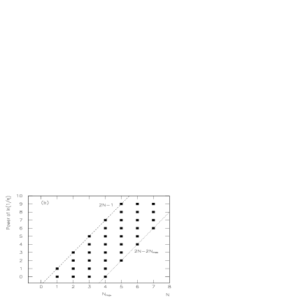
Figure 8: Resummation of Eq. (19). Each point corresponds to a contribution (19). The points along the straight line ‘power of $\ln\big{(}{1\over\eta}\big{)}=2N$’ represent terms coming from the Sudakov factor. Figures (b) and (d) illustrate contributions summed when this factor is expanded. In particular, here $N_{\rm max}=4$ and $m_{\rm max}=7$ for the case (a),(b) and $m_{\rm max}=1$ in (c), (d). Note that only the $N_{\rm max}$, min$(N_{\rm max},2+2m_{\rm max})$ first ‘towers’ are fully summed in (b), (d), respectively.

The terms which contribute to the new series (18) are illustrated schematically in Fig. 8. Notice that the extraction of the Sudakov factor results in an ability to sum an infinite subseries of logarithms. This observation constitutes a basis for our further analysis. However, there is a shortcoming: in order to sum the first $m$ ‘towers’ fully we need to take $N_{\rm max}=m$ which leads us to include extra sub-leading contributions from more than the first $m$ ‘towers’, cf. Fig. 8b.

The individual contributions to the summation (18),

$${1\over\eta}e^{-{\lambda\over 2}\ln^{2}\big{(}{1\over\eta}\big{)}}{(-2)^{(N-1)}\lambda^{N}\over m!(N-1-m)!}\ln^{N-1-m}\bigg{(}{1\over\eta}\bigg{)}\bigg{[}2\bar{b}_{N+m}(\infty)+\ln\bigg{(}{1\over\eta}\bigg{)}\bar{b}_{N+m-1}(\infty)\bigg{]}\ ,$$ (19)

are presented in Fig. 7. As was the case for (14), the importance of the $\ln\left({1\over\eta}\right)$ factors diminishes for small $m$ and large $\eta$. Note that for small $\eta$ the sizes of the contributions are much smaller here than for (10).

Next we perform the same analysis as for (10), i.e. we study the dependence of (18) on $N_{\rm max}$ and on the ‘cut-off’ value $m_{\rm max}$. Comparing the cumulative plot for (18), Fig. 9, with Fig. 6, we note that the $b$-space result is now better approached close to the line $m_{\rm max}=N_{\rm max}-1$ (such an effect can be observed in the case of (10) only for large $\eta$). When $m_{\rm max}<N_{\rm max}-1$ the balance between different contributions is apparently spoiled until $m_{\rm max}$ becomes considerably small. Again, it turns out that it is necessary to incorporate the first few sub-leading kinematic logarithmic terms (i.e. some moderate $N_{\rm max}$) to obtain the best approximation of the $b$-space result.

The asymptotic properties of (18) can be most easily seen for large values of $\eta$ and large $N_{\rm max}$. The apparent discrepancy between the $b$-space result and the summation (18) is caused here by contributions with $m=N-1$, i.e. terms proportional to $\bar{b}_{2N-1}(\infty)$. The other terms are negligible as they contain powers of $\ln\left({1\over\eta}\right)$ which for these $\eta$ are very small. The dominant contribution is then proportional to $(-1)^{N_{\rm max}-1}2^{N_{\rm max}}\bar{b}_{2N_{\rm max}-1}(\infty)/(N_{\rm max}-1)!$, i.e. the sign varies as $(-1)^{N_{\rm max}}$. Fortunately, the range of $\eta$ for which the discrepancy occurs is outside the region of interest for the present discussion. Also, in practice we never take $N_{\rm max}$ so large as to make this effect substantial. Nevertheless, it emphasises the necessity of performing a careful matching with the fixed-order perturbative result.

We may therefore conclude that the expression (18), with the Sudakov factor resummed and factored out, enables us to resum infinite series of logarithms while at the same time allows for the inclusion of kinematical sub-leading logarithms. Moreover, it has very good convergence properties over a large range of $\eta$, while summing leading and sub-leading logarithmic terms. It is thus well suited for the purposes of this analysis, i.e. reproducing the $b$-space result by explicit resummation in $q_{T}$ space, and we will continue to use it for the rest of this study.

3.2 Running coupling analysis

The ultimate goal of the work presented here is to obtain a more accurate description, if possible, of the $W$ production distribution. To this end, one has to incorporate various other sub-leading effects in addition to the kinematic logarithms discussed in the previous subsection. One example is the incorporation of the running of the strong coupling $\alpha_{S}$ into the cross section expression. This is achieved by substituting

$$\alpha_{S}(\bar{\mu}^{2})=\alpha_{S}(\mu^{2}) \bigg{\{} \!\!1-{\alpha_{S}(\mu^{2})\over\pi}\beta_{0}\ln({\bar{\mu}^{2}\over\mu^{2}})$$ (20)

$$+{\alpha_{S}(\mu^{2})^{2}\over\pi^{2}}\ln({\bar{\mu}^{2}\over\mu^{2}})\left(\beta_{0}^{2}\ln({\bar{\mu}^{2}\over\mu^{2}})-\beta_{1}\right)\bigg{\}}+{\cal O}(\alpha_{S}^{3}(\mu^{2}))\,,$$

with

$$\beta_{0}={1\over 4}\left(11-{2\over 3}n_{f}\right)\,,\qquad\beta_{1}={1\over 16}\left(102-{38\over 3}n_{f}\right)\,,$$ (21)

in (18). The effect on the DLLA form factor is to introduce a sequence of sub-leading logarithms whose coefficients depend on the $\beta$–function coefficients defined in (20). If only the 1-loop running of $\alpha_{S}$ is introduced then the cross section expression (18) reads

$${1\over\sigma_{0}}{d\sigma\over d\eta} ={\alpha_{S}(\mu^{2})A^{(1)}\over 2\pi\eta}e^{-{\alpha_{S}(\mu^{2})A^{(1)}\over 4\pi}\ln^{2}\big{(}{1\over\eta}\big{)}\big{[}1+{1\over 3\pi}\beta_{0}\alpha_{S}(\mu^{2})\big{(}2\ln\big{(}{1\over\eta}\big{)}-3\ln\big{(}{Q^{2}\over\mu^{2}}\big{)}\big{)}\big{]}}$$ (27)

$$\times\sum_{N=1}^{\infty}\Bigg{(}-{\alpha_{S}(\mu^{2})A^{(1)}\over\pi}\Bigg{)}^{N-1}{1\over(N-1)!}\sum_{m=0}^{N-1}{\left(\begin{array}[]{c}N-1\\ m\end{array}\right)}\sum_{k=0}^{N-m-1}{\left(\begin{array}[]{c}N-m-1\\ k\end{array}\right)}$$

$$c_{2}^{m}c_{3}^{k}c_{1}^{N-m-k-1}\times\bigg{[}3c_{3}\bar{b}_{N+m+2k+1}(\infty)+2c_{2}\bar{b}_{N+m+2k}(\infty)+c_{1}\bar{b}_{N+m+2k-1}(\infty)\bigg{]}\,,\qquad$$

with

$$c_{3}={4\over 3\pi}\beta_{0}\alpha_{S}(\mu^{2})\,,$$

$$c_{2}={1\over\pi}\bigg{[}\pi+\beta_{0}\alpha_{S}(\mu^{2})\bigg{(}2\ln\bigg{(}{1\over\eta}\bigg{)}-\ln\bigg{(}{Q^{2}\over\mu^{2}}\bigg{)}\bigg{)}\bigg{]}\,,$$

$$c_{1}={1\over\pi}\ln\bigg{(}{1\over\eta}\bigg{)}\bigg{[}\pi+\beta_{0}\alpha_{S}(\mu^{2})\bigg{(}\ln\bigg{(}{1\over\eta}\bigg{)}-\ln\bigg{(}{Q^{2}\over\mu^{2}}\bigg{)}\bigg{)}\bigg{]}\,.$$ (28)

Notice the appearance in (27) of sub-leading ${\cal O}(\alpha_{S}^{2}\ln^{3}(1/\eta))$ terms in the exponent of the Sudakov form factor. Interestingly, these logarithms can be eliminated by a particular scale choice: $\mu^{2}=Q^{2}\,\eta^{2/3}$. This restores the same form as in (18) i.e. $\exp{\big{(}-{\alpha_{S}A^{(1)}\over\pi}\ln^{2}\big{(}{1\over\eta}\big{)}\big{)}}$, but now with a coupling which also depends on $\eta$. However not all $\beta_{0}$–dependent logarithms are eliminated. For example, we can see from (28) that corrections of order $\beta_{0}\alpha_{S}\ln\big{(}{1\over\eta}\big{)}$ remain. Of course in a complete calculation the dependence on the scale choice should disappear. To illustrate the residual dependence on the scale of the cross section (27) we show (Fig. 10) results for two different choices: $\mu^{2}=\eta\,Q^{2}=q_{T}^{2}$ and $\mu^{2}=Q^{2}\,\eta^{2/3}$. Also shown is the effect of truncating the sum in (27) at first, second and third order.

We see that with $\mu^{2}=Q^{2}\,\eta^{2/3}$ there is slightly less stability with respect to the truncation point than there is with the choice $\mu^{2}=q_{T}^{2}$. Note also that now the plots of ${1\over\sigma_{0}}{d\sigma\over d\eta}$ are no longer explicitly independent of $Q$, as was the case when $\alpha_{S}$ was taken to be constant. The additional dependence on $Q$ enters into (27) via the coupling $\alpha_{S}(\mu^{2})=\alpha_{S}(Q^{2/3}q_{T}^{4/3})$. For values of $q_{T}$ where perturbative QCD can safely be applied (e.g. $q_{T}\geq 3$ GeV) and the energies considered here, the resulting scale $\mu$ is bigger than the $b$ quark mass, and we therefore avoid evolving the coupling through any quark mass thresholds.

An extension of this analysis for the case of the two-loop running coupling is straightforward and gives

$${1\over\sigma_{0}}{d\sigma\over d\eta} ={\alpha_{S}(\mu^{2})A^{(1)}\over 2\pi\eta}e^{S_{\eta}}\sum_{N=1}^{\infty}\Bigg{(}-{\alpha_{S}(\mu^{2})A^{(1)}\over\pi}\Bigg{)}^{N-1}{1\over(N-1)!}\sum_{m=0}^{N-1}{\left(\begin{array}[]{c}N-1\\ m\end{array}\right)}$$ (37)

$$\times\sum_{k=0}^{N-m-1}{\left(\begin{array}[]{c}N-m-1\\ k\end{array}\right)}\sum_{l=0}^{N-m-k-1}{\left(\begin{array}[]{c}N-m-k-1\\ l\end{array}\right)}c_{2}^{m}c_{3}^{k}c_{4}^{l}c_{1}^{N-m-k-l-1}$$

$$\times\bigg{[}4c_{4}\bar{b}_{N+m+2k+3l+2}(\infty)+3c_{3}\bar{b}_{N+m+2k+3l+1}(\infty)+2c_{2}\bar{b}_{N+m+2k+3l}(\infty)$$

$$\ +c_{1}\bar{b}_{N+m+2k+3l-1}(\infty)\bigg{]}\,.$$

Here

$$S_{\eta} = -{\alpha_{S}(\mu^{2})A^{(1)}\over 4\pi}\ln^{2}\bigg{(}{1\over\eta}\bigg{)}\bigg{[}1+{1\over 3\pi}\bigg{(}\beta_{0}\alpha_{S}(\mu^{2})+{1\over\pi}\beta_{1}\alpha_{S}^{2}(\mu^{2})\bigg{)}\bigg{(}2\ln\bigg{(}{1\over\eta}\bigg{)}-3\ln\bigg{(}{Q^{2}\over\mu^{2}}\bigg{)}\bigg{)}$$

$$+{1\over 6\pi^{2}}\alpha_{S}^{2}(\mu^{2})\beta_{0}^{2}\bigg{(}3\ln^{2}\bigg{(}{1\over\eta}\bigg{)}-8\ln\bigg{(}{1\over\eta}\bigg{)}\ln\bigg{(}{Q^{2}\over\mu^{2}}\bigg{)}+6\ln^{2}\bigg{(}{Q^{2}\over\mu^{2}}\bigg{)}\bigg{)}\bigg{]}\,,$$

$$c_{4} = {2\over\pi^{2}}\alpha_{S}^{2}(\mu^{2})\beta_{0}^{2}\,,$$

$$c_{3} = {4\over 3\pi^{2}}\bigg{[}\beta_{0}\alpha_{S}(\mu^{2})\pi+\beta_{1}\alpha_{S}^{2}(\mu^{2})+\beta_{0}^{2}\alpha_{S}^{2}(\mu^{2})\bigg{(}3\ln\bigg{(}{1\over\eta}\bigg{)}-2\ln\bigg{(}{Q^{2}\over\mu^{2}}\bigg{)}\bigg{)}\bigg{]}\,,$$

$$c_{2} = {1\over\pi^{2}}\bigg{[}\pi^{2}+\bigg{(}\beta_{0}\alpha_{S}(\mu^{2})\pi+\beta_{1}\alpha_{S}^{2}(\mu^{2})\bigg{)}\bigg{(}2\ln\bigg{(}{1\over\eta}\bigg{)}-\ln\bigg{(}{Q^{2}\over\mu^{2}}\bigg{)}\bigg{)}$$

$$+\beta_{0}^{2}\alpha_{S}^{2}(\mu^{2})\bigg{(}3\ln^{2}\bigg{(}{1\over\eta}\bigg{)}-4\ln\bigg{(}{1\over\eta}\bigg{)}\ln\bigg{(}{Q^{2}\over\mu^{2}}\bigg{)}+\ln^{2}\bigg{(}{Q^{2}\over\mu^{2}}\bigg{)}\bigg{)}\bigg{]}\,,$$

$$c_{1} = {1\over\pi^{2}}\ln\bigg{(}{1\over\eta}\bigg{)}\bigg{[}\pi^{2}+\bigg{(}\beta_{0}\alpha_{S}(\mu^{2})\pi+\beta_{1}\alpha_{S}^{2}(\mu^{2})\bigg{)}\bigg{(}\ln\bigg{(}{1\over\eta}\bigg{)}-\ln\bigg{(}{Q^{2}\over\mu^{2}}\bigg{)}\bigg{)}$$

$$+\beta_{0}^{2}\alpha_{S}^{2}(\mu^{2})\bigg{(}\ln^{2}\bigg{(}{1\over\eta}\bigg{)}-2\ln\bigg{(}{1\over\eta}\bigg{)}\ln\bigg{(}{Q^{2}\over\mu^{2}}\bigg{)}+\ln^{2}\bigg{(}{Q^{2}\over\mu^{2}}\bigg{)}\bigg{)}\bigg{]}\,.$$

Now, after fixing the choice of scale as described above, a new term proportional to $\beta_{0}^{2}\alpha_{S}^{3}(\mu^{2})\ln^{4}\big{(}{1\over\eta}\big{)}$ appears in the exponential. As a result, the line of points corresponding to terms of the form $\alpha_{S}^{N}\ln^{2N-1}\big{(}{1\over\eta}\big{)}$ in Fig. 8a will now change to the set of points corresponding to $\alpha_{S}^{3N}\ln^{4N}\big{(}{1\over\eta}\big{)}$ or higher powers of $\ln\big{(}{1\over\eta}\big{)}$. Unlike the $\ln^{3}\big{(}{1\over\eta}\big{)}$ terms, those with $\ln^{4}\big{(}{1\over\eta}\big{)}$ do not cancel when $\mu^{2}=Q^{2/3}q_{T}^{4/3}$ is chosen. It is impossible to cancel these terms by any choice of the renormalization scale. On the other hand, the choice which eliminates those terms with $\ln^{3}\big{(}{1\over\eta}\big{)}$ is also the one that minimizes the coefficient of the $\ln^{4}\big{(}{1\over\eta}\big{)}$ terms.

3.3 Resummation including all types of sub-leading logarithms

A derivation of the expression for the cross section for the case when all known leading and sub-leading coefficients, i.e. $A^{(1)},B^{(1)},A^{(2)},B^{(2)}$, are taken into account follows the method introduced above and gives (fixed coupling to begin with)

$${1\over\sigma_{0}}{d\sigma\over d\eta} ={\alpha_{S}A^{(1)}\over 2\pi\eta}e^{S_{\eta}}\sum_{N=1}^{\infty}{\Bigg{(}-{\alpha_{S}A^{(1)}\over\pi}\Bigg{)}^{N-1}}{1\over(N-1)!}\sum_{m=0}^{N-1}{\left(\begin{array}[]{c}N-1\\ m\end{array}\right)}$$ (41)

$$\times c_{2}^{m}c_{1}^{N-m-1}\bigg{[}2c_{2}\bar{b}_{N+m}(\infty)+c_{1}\bar{b}_{N+m-1}(\infty)\bigg{]}\,,$$

with

$$S_{\eta} = -{\alpha_{S}A^{(1)}\over 4\pi}\bigg{[}\ln^{2}\bigg{(}{1\over\eta}\bigg{)}\bigg{(}1+{\alpha_{S}\over 2\pi}{A^{(2)}\over A^{(1)}}\bigg{)}+\ln\bigg{(}{1\over\eta}\bigg{)}\bigg{(}2{B^{(1)}\over A^{(1)}}+{\alpha_{S}\over\pi}{B^{(2)}\over A^{(1)}}\bigg{)}\bigg{]}\,,$$

$$c_{1} = \bigg{(}1+{\alpha_{S}\over 2\pi}{A^{(2)}\over A^{(1)}}\bigg{)}\ln\bigg{(}{1\over\eta}\bigg{)}+{B^{(1)}\over A^{(1)}}+{\alpha_{S}\over 2\pi}{B^{(2)}\over A^{(1)}}\,,$$

$$c_{2} = 1+{\alpha_{S}\over 2\pi}{A^{(2)}\over A^{(1)}}\,.$$

Now each logarithmic term in the sum (41) acquires a factor which is a combination of the $A$s, $B$s and $\bar{b}(\infty)$’s. Notice that although the various sub-leading logarithms are mixed together, they have a distinctive origin. We have mentioned already that the DLLA (i.e. retaining only terms of the form $A^{(1)}\alpha_{S}^{N}\ln^{2N-1}\big{(}{1\over\eta}\big{)}$ ) corresponds to the situation where all gluons are soft and collinear and where strong ordering of the transverse momenta and energies is imposed. We also know that other terms with $A^{(1)}$ multiplied by the $\bar{b}_{m}(\infty)$ arise from using the soft and collinear approximation for the matrix element but relaxing the strong-ordering condition. The sub-leading terms with $B^{(1)}$ etc. correspond to the situation where at least one gluon is either non-collinear or energetic.

In addition, extracting a Sudakov form factor from the sum (41) ‘squeezes’ it down to a summation over $m$ from 0 to $N-1$, thereby reducing the number of fully known ‘towers’ of logarithms: from the first four to the first two. This can be appreciated by comparing the logarithmic coefficients appearing in the expansion of the cross section up to and including the first three orders in $\alpha_{S}$ with (Table 3) and without (Table 2) the Sudakov form factor extracted.

These tables also reveal another relevant property: sub-leading coefficients like $A^{(2)}$ are associated with $\bar{b}(\infty)$ factors whose indices are not as high as those which accompany $A^{(1)}$. Both $\ln{\big{(}{1\over\eta}\big{)}}$ terms and $\bar{b}(\infty)$ factors originate from the same $\ln\big{(}{Q^{2}b^{2}\over b_{0}^{2}}\big{)}$ terms appearing at the very early stage of the derivation. In particular, let us focus on a term with a particular power of $\alpha_{S}$ and $\ln{\big{(}{1\over\eta}\big{)}}$. To reproduce such a term one has to take $\ln\big{(}{Q^{2}b^{2}\over b_{0}^{2}}\big{)}$ up to the appropriate power, depending on its associated coefficient (i.e. $A$ or $B$). For sub-leading coefficients this power will be obviously lower than for more leading ones. Hence the indices of the corresponding $\bar{b}(\infty)$ factors are lower for more sub-leading coefficients. For example, the index of $\bar{b}(\infty)$ accompanying the first sub-leading unknown coefficient $A^{(3)}$ would be at least four less than the index of a corresponding $\bar{b}(\infty)$ for the $A^{(1)}$ coefficient, for given powers of $\alpha_{S}$ and $\ln{\big{(}{1\over\eta}\big{)}}$. This observation provides us with a strong argument for justifying the inclusion of known parts of logarithmic terms from sub-leading ‘towers’ lower than NNNL. Physically, the $\bar{b}(\infty)$ factors are of kinematic origin and as such they are much more relevant to the cross section than perturbative lower order coefficients in the expansion of $A(\alpha_{S}(\mu^{2}))$ and $B(\alpha_{S}(\mu^{2}))$. While, as we have shown earlier, resummation of the terms containing $\bar{b}(\infty)$ factors with higher indices can still be of numerical importance for the final result, terms with unknown higher-order perturbative coefficients seem to contribute corrections of much smaller size.

A comparison of effects induced by the inclusion of successive sub-leading coefficients in (41) is demonstrated in Fig. 11. Also shown are the results of an exact integration in $b$-space. The agreement for low values of $\eta$ is excellent. At high $\eta$ we encounter a discrepancy of the same nature as that discussed for the case of the leading coefficient $A^{(1)}$, i.e. for large $N_{\rm max}$ the expression (41) either grows significantly or acquires negative values, depending on the number of terms at which the expression is truncated. For the values of $N_{\rm max}$ we use in our calculations this behaviour does not occur.

With the above prescriptions for the sub-leading logarithmic terms, kinematic effects and running coupling, we finally obtain a ‘complete’ expression for the cross section:

$${1\over\sigma_{0}}{d\sigma\over d\eta} ={\alpha_{S}(\mu^{2})A^{(1)}\over 2\eta\pi}e^{S_{\eta}}\sum_{N=1}^{\infty}\Bigg{(}{-\alpha_{S}(\mu^{2})A^{(1)}\over\pi}\Bigg{)}^{N-1}{1\over(N-1)!}\sum_{m=0}^{N-1}{\left(\begin{array}[]{c}N-1\\ m\end{array}\right)}$$ (44)

$$\times \sum_{k=0}^{N-m-1}{\left(\begin{array}[]{c}N-m-1\\ k\end{array}\right)}\sum_{l=0}^{N-m-k-1}{\left(\begin{array}[]{c}N-m-k-1\\ l\end{array}\right)}$$ (49)

$$\times \sum_{j=0}^{N-m-k-l-1}{\left(\begin{array}[]{c}N-m-k-l-1\\ j\end{array}\right)}\sum_{i=0}^{N-m-k-l-j-1}{\left(\begin{array}[]{c}N-m-k-l-j-1\\ i\end{array}\right)}$$ (54)

$$\times c_{2}^{m}c_{3}^{k}c_{4}^{l}c_{5}^{j}c_{6}^{i}c_{1}^{N-m-k-l-j-i-1}\sum_{n=1}^{6}nc_{n}\bar{b}_{N+m+2k+3l+4j+5i+n-2}(\infty)\,.$$ (55)

The expressions for $S_{\eta}$ and the $c_{i}$ are now of course much more complicated. Explicit expressions up to fifth order in the coupling constant $\alpha_{S}(\mu^{2})$ are presented in the Appendix. The fifth order appears here as a consequence of using the two-loop expansion of the running coupling and including the first four terms in the expansion of $S_{\eta}$ (4).

Numerical results based on the complete expression are displayed in Figs. 12-13, for the scale choice $\mu^{2}=Q^{2/3}q_{T}^{4/3}$. First, Fig. 12 shows the cross section with all four $A_{i},\;B_{i}$ coefficients included, together with the first three orders in $\alpha_{S}(\mu^{2})$ in the entire sum over $N$ in (55). Notice the rapid convergence when the higher-orders are included. Fig. 13 shows how the first-order cross section is influenced by the various $A_{i},\;B_{i}$ coefficients. Notice how the relative impact on the leading-order $A_{1}$ result is essentially $B_{1}>A_{2}>B_{2}$, as might be expected. The effect of including $B_{2}$ is numerically small, indicating a reasonable degree of convergence from the higher-order coefficients.

The result (55) is valid in general for any choice of the renormalization scale $\mu$. However, the expressions for $S_{\eta}$ and the $c$’s will change depending on the particular scale choice. For $\mu^{2}=Q^{2}$ the expression for the cross section ${1\over\sigma_{0}}{d\sigma\over d\eta}$ corresponds to $F^{(q_{T})}(q_{T})$ in Ref. [5]. More precisely, $F^{(q_{T})}(q_{T})$ as defined in [5] can be obtained from (55) by choosing an upper limit of summation $N=5$ and putting $\bar{b}_{i}(\infty)=0$ for $i\geq 1$. This recipe comes from the observation that the only coefficient appearing together with $\bar{b}_{0}(\infty)$ is $c_{1}$, which contains terms up to ${\cal{O}}(\alpha_{S}^{5}(Q^{2}))$. Moreover, the expression (55), when calculated for $\mu^{2}=Q^{2}$ and expanded in powers of $\alpha_{S}(Q^{2})$ gives the ${\cal{O}}(\alpha_{S}^{2}(Q^{2}))$ ‘perturbation theory’ result $F^{(p)}(q_{T})$ from [5]. In Fig. 14 we show $F^{(p)}(q_{T})$ and $F^{(q_{T})}(q_{T})$ as functions of $q_{T}$, analogous to Fig. 3 in [5].

The $q_{T}$-space formalism as presented in [5] does not take account of non-zero $\bar{b}_{i}(\infty)$ with $i\geq 1$, and therefore does not include known contributions from sub-leading NNNL ‘towers’ of (kinematic) logarithms. This is partially compensated for in [5] by a redefinition of $B^{(2)}$,

$$\tilde{B}^{(2)}=B^{(2)}+2A^{(1)}\zeta(3)$$ (56)

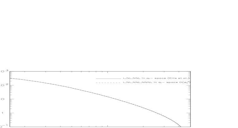
Figure 16: Resummation of the first three (L,NL,NNL) ‘towers’ according to [5] and the first four (L,NL,NNL,NNNL) towers of logarithms (55) for $\mu^{2}=Q^{2}$, $Q=M_{Z}=91.187$ GeV, $\alpha_{S}(M_{Z}^{2})=0.113$.

which, although it does correctly account for a ${\cal{O}}(\alpha_{S}^{2}(Q^{2}))$ term from the NNNL ‘tower’ (see Table 2), distorts other terms from this ‘tower’. With the help of our expression (55) we can obtain the first four ‘towers’ fully resummed. It should however be remembered that the result is not ‘pure’, in the sense that it contains additional sub-leading terms. On the other hand, an effect induced by the redefinition of $B^{(2)}$ seems to be comparable with that caused by summing these sub-leading terms in (55) (with non-zero $\bar{b}_{3}(\infty)$, $\bar{b}_{5}(\infty))$, see Fig. 15. A difference obviously arises when the fourth tower is also resummed (cf. Fig. 16) — numerically we encounter an increase in the cross section of approximately 3% for all values of $q_{T}$, when the scale equals $\mu^{2}=Q^{2}$. Furthermore, Fig. 17 shows the effect of including 3,5,6,7,8 ‘towers’, normalised to the 4th-tower result, now for the scale choice $\mu^{2}=Q^{2/3}q_{T}^{4/3}$. The figure clearly shows the numerical importance of the kinematical logarithms of the higher towers, and also the stability over a broad range of relevant $q_{T}$ as more towers are included. However, this change is approximately of the same magnitude as the one observed for the change of the renormalization scale. In particular, for the 4 towers of logarithms, changing the scale from our default $\mu^{2}=Q^{2/3}q_{T}^{4/3}$ to the (lower) scale $\mu^{2}=q_{T}^{2}$ and the (higher) scale $\mu^{2}=Q^{2}$ changes the $q_{T}$ distribution by less than $\pm 3\%$ over the complete low-$q_{T}$ range.

4 Summary and conclusions

The $q_{T}$-space formalism for describing vector boson production in hadron collisions is known to overcome many of the problems faced by the $b$-space method. In this paper we have further investigated the $q_{T}$-space approach. For the parton-level subprocess cross section we have modified the existing approach in order to incorporate sub-leading ‘kinematic’ logarithms. We have carefully studied the effect of various sub-leading contributions: higher-order perturbative coefficients, the running coupling, and the ‘kinematic’ logarithms. We have confirmed that the ‘kinematic’ logarithms are particularly important at small $q_{T}$, where they serve to cancel the suppressing effect of the Sudakov form factor.

Our technique enables us to resum the first four logarithmic ‘towers’ including the NNNL series, together with the first few sub-leading ‘kinematic’ logarithms. We have shown that that the most significant quantitative change in the predictions for the cross section is caused by resumming the NNNL ‘tower’. The fact that the fourth ‘tower’ only changes the cross section by about $3\%$ shows that the convergence of our expansion is certainly adequate for phenomenological applications. We note that a drawback of this method is an inability to select a particular numbers of ‘towers’ to be fully resummed.

In this paper we have concentrated only on the perturbative contributions to the cross section. It is well known that in practice non-perturbative effects (‘$k_{T}$ smearing’) are also important, and affect the $W$ $q_{T}$ distribution in the very low $q_{T}$ region, see for example Ref. [4]. These must be taken into account before assessing the impact of the sub-leading logarithmic contributions on the physical cross section. We will address these issues in a forthcoming study.

Note added: As this paper was nearing completion we became aware of an interesting new study of soft gluon resummation, Ref. [10], which addresses the same problem. In Ref. [10], resummation in $b$-space is studied, in particular the impact of factorially growing terms in the $\alpha_{s}$ expansion therein. A closed expression is subsequently obtained for the corresponding $q_{T}$ space result, which resums logarithms at the NLL level in the Sudakov exponent. The kinematic logarithms are also treated differently, such that a singularity is encountered as $q_{T}\to q_{T}^{\rm crit}>0$. We will compare the phenomenological implications of the two approaches in a forthcoming study.

Acknowledgments
This work was supported in part by the EU Fourth Framework Programme ‘Training and Mobility of Researchers’, Network ‘Quantum Chromodynamics and the Deep Structure of Elementary Particles’, contract FMRX-CT98-0194 (DG 12 - MIHT). A.K. gratefully acknowledges financial support received from the Overseas Research Students Award Scheme and the University of Durham.

Appendix

In this appendix we list the expressions for $S_{\eta}$ and the $c_{i}$ coefficients in (55), for the choice of the renormalization scale $\mu^{2}=Q^{2}\eta^{2/3}$.

$$S_{\eta}=-{\frac{1}{2}}\lambda\Bigg{[}{\frac{1}{270}}\,{\frac{\alpha_{S}(\mu^{2})^{5}\,{\beta_{0}}^{4}\,A^{(2)}\,{\rm ln}\bigg{(}{\frac{1}{\eta}}\bigg{)}^{6}\,}{\pi^{5}\,A^{(1)}}}+\bigg{(}-{\frac{1}{135}}\,{\frac{{\beta_{0}}^{3}\,\alpha_{S}(\mu^{2})^{4}\,A^{(2)}}{\pi^{4}\,A^{(1)}}}$$

$$-4\,\pi\,\bigg{(}{\frac{1}{540}}\,{\frac{{\beta_{0}}^{2}\,{\beta_{1}}\,A^{(2)}}{\pi^{6}\,A^{(1)}}}-{\frac{11}{1620}}\,{\frac{{\beta_{0}}^{4}\,B^{(2)}}{\pi^{6}\,A^{(1)}}}\bigg{)}\,\alpha_{S}(\mu^{2})^{5}\bigg{)}\,{\rm ln}\bigg{(}{\frac{1}{\eta}}\bigg{)}^{5}$$

$$+\bigg{(}{\frac{1}{12}}\,{\frac{{\beta_{0}}^{2}\,\alpha_{S}(\mu^{2})^{3}\,A^{(2)}}{\pi^{3}\,A^{(1)}}}-4\,\pi\,\bigg{(}-{\frac{1}{144}}\,{\frac{{\beta_{1}}^{2}\,A^{(2)}}{\pi^{6}\,A^{(1)}}}+{\frac{5}{216}}\,{\frac{{\beta_{0}}^{2}\,{\beta_{1}}\,B^{(2)}}{\pi^{6}\,A^{(1)}}}\bigg{)}\,\alpha_{S}(\mu^{2})^{5}$$

$$\mbox{}-4\,\pi\,\bigg{(}-{\frac{1}{72}}\,{\frac{{\beta_{0}}\,{\beta_{1}}\,A^{(2)}}{\pi^{5}\,A^{(1)}}}+{\frac{5}{216}}\,{\frac{{\beta_{0}}^{3}\,B^{(2)}}{\pi^{5}\,A^{(1)}}}\bigg{)}\,\alpha_{S}(\mu^{2})^{4}+{\frac{1}{18}}\,{\frac{{\beta_{0}}^{2}\,\alpha_{S}(\mu^{2})^{2}}{\pi^{2}}}\bigg{)}{\rm ln}\bigg{(}{\frac{1}{\eta}}\bigg{)}^{4}$$

$$\mbox{}+\bigg{(}{\frac{1}{9}}\,{\frac{{\beta_{1}}^{2}\,\alpha_{S}(\mu^{2})^{5}\,B^{(2)}}{\pi^{5}\,A^{(1)}}}+{\frac{2}{9}}\,{\frac{{\beta_{0}}\,{\beta_{1}}\,\alpha_{S}(\mu^{2})^{4}\,B^{(2)}}{\pi^{4}\,A^{(1)}}}+{\frac{1}{3}}\,{\frac{{\beta_{0}}^{2}\,\alpha_{S}(\mu^{2})^{3}\,B^{(2)}}{\pi^{3}\,A^{(1)}}}+{\frac{2}{9}}\,{\frac{\alpha_{S}(\mu^{2})^{2}\,{\beta_{0}}^{2}\,B^{(1)}}{\pi^{2}\,A^{(1)}}}\bigg{)}$$

$$\times\,{\rm ln}\bigg{(}{\frac{1}{\eta}}\bigg{)}^{3}+\bigg{(}-{\frac{1}{3}}\,{\frac{{\beta_{1}}\,\alpha_{S}(\mu^{2})^{3}\,B^{(2)}}{\pi^{3}\,A^{(1)}}}-4\,\pi\,\bigg{(}{\frac{1}{12}}\,{\frac{{\beta_{0}}\,B^{(2)}}{\pi^{3}\,A^{(1)}}}+{\frac{1}{12}}\,{\frac{{\beta_{1}}\,B^{(1)}}{\pi^{3}\,A^{(1)}}}\bigg{)}\,\alpha_{S}(\mu^{2})^{2}$$

$$-4\,\pi\,\bigg{(}-{\frac{1}{8}}\,{\frac{A^{(2)}}{\pi^{2}\,A^{(1)}}}+{\frac{1}{12}}\,{\frac{{\beta_{0}}\,B^{(1)}}{\pi^{2}\,A^{(1)}}}\bigg{)}\,\alpha_{S}(\mu^{2})\mbox{}+1\bigg{)}{\rm ln}\bigg{(}{\frac{1}{\eta}}\bigg{)}^{2}\mbox{}+\bigg{(}{\frac{\alpha_{S}(\mu^{2})\,B^{(2)}}{\pi\,A^{(1)}}}+2\,{\frac{B^{(1)}}{A^{(1)}}}\bigg{)}\,{\rm ln}\bigg{(}{\frac{1}{\eta}}\bigg{)}\bigg{]}\,,$$

$${c_{1}}=\left({\vrule height=13.60002pt,width=0.0pt,depth=13.60002pt}\right.\!\!{\frac{1}{18}}\,{\frac{\beta_{1}^{2}\,B^{(2)}\,{\rm ln}\bigg{(}{\frac{1}{\eta}}\bigg{)}^{2}}{\pi^{5}\,A^{(1)}}}+{\frac{1}{30}}\,{\frac{\bigg{(}{\frac{10}{9}}\,{\frac{\beta_{0}^{2}\,\beta_{1}\,B^{(2)}}{A^{(1)}}}+{\frac{5}{3}}\,{\frac{\beta_{1}^{2}\,A^{(2)}}{A1^{(1)}}}\bigg{)}\,{\rm ln}\bigg{(}{\frac{1}{\eta}}\bigg{)}^{3}}{\pi^{5}}}$$

$$\mbox{}+{\frac{1}{30}}\,{\frac{\bigg{(}{\frac{5}{27}}\,{\frac{\beta_{0}^{4}\,B^{(2)}}{A^{(1)}}}+{\frac{10}{9}}\,{\frac{\beta_{0}^{2}\,\beta_{1}\,A^{(2)}}{A^{(1)}}}\bigg{)}\,{\rm ln}\bigg{(}{\frac{1}{\eta}}\bigg{)}^{4}}{\pi^{5}}}+{\frac{1}{162}}\,{\frac{{\rm ln}({\frac{1}{\eta}})^{5}\,\beta_{0}^{4}\,A^{(2)}}{\pi^{5}\,A^{(1)}}}\!\!\left.{\vrule height=13.60002pt,width=0.0pt,depth=13.60002pt}\right)\alpha_{S}(\mu^{2})^{5}\mbox{}$$

$$+\left(\!{\frac{1}{9}}\,{\frac{\beta_{0}\,\beta_{1}\,B^{(2)}\,{\rm ln}\bigg{(}{\frac{1}{\eta}}\bigg{)}^{2}}{\pi^{4}\,A^{(1)}}}+{\frac{1}{27}}\,{\frac{\beta_{0}^{3}\,A^{(2)}\,{\rm ln}\bigg{(}{\frac{1}{\eta}}\bigg{)}^{4}}{\pi^{4}\,{\it A^{(1)}}}}+{\frac{1}{30}}\,{\frac{\bigg{(}{\frac{10}{9}}\,{\frac{\pi\,\beta 0^{3}\,B^{(2)}}{A^{(1)}}}+{\frac{10}{3}}\,{\frac{\pi\,\beta_{0}\,\beta_{1}\,A^{(2)}}{A^{(1)}}}\bigg{)}\,{\rm ln}\bigg{(}{\frac{1}{\eta}}\bigg{)}^{3}}{\pi^{5}}}\!\right)\alpha_{S}(\mu^{2})^{4}$$

$$\mbox{}+\left(\!{\frac{1}{3}}\,{\frac{\beta_{1}\,B^{(2)}\,{\rm ln}\bigg{(}{\frac{1}{\eta}}\bigg{)}}{\pi^{3}\,A^{(1)}}}+{\frac{1}{30}}\,{\frac{\bigg{(}5\,{\frac{\pi^{2}\,\beta_{0}^{2}\,B^{(2)}}{A^{(1)}}}+10\,{\frac{\pi^{2}\,\beta_{1}\,A^{(2)}}{A^{(1)}}}\bigg{)}\,{\rm ln}\bigg{(}{\frac{1}{\eta}}\bigg{)}^{2}}{\pi^{5}}}+{\frac{1}{6}}\,{\frac{\beta_{0}^{2}\,A^{(2)}\,{\rm ln}\bigg{(}{\frac{1}{\eta}}\bigg{)}^{3}}{\pi^{3}\,A^{(1)}}}\!\right)\,\alpha_{S}(\mu^{2})^{3}$$

$$+\left({\vrule height=13.60002pt,width=0.0pt,depth=13.60002pt}\right.\!\!{\frac{1}{30}}\,{\frac{\bigg{(}10\,{\frac{\pi^{3}\,\beta_{0}\,B^{(2)}}{A^{(1)}}}+10\,{\frac{\pi^{3}\,\beta_{1}\,B^{(1)}}{A^{(1)}}}\bigg{)}\,{\rm ln}\bigg{(}{\frac{1}{\eta}}\bigg{)}}{\pi^{5}}}$$

$$\mbox{}+{\frac{1}{30}}\,{\frac{\bigg{(}{\frac{10}{3}}\,{\frac{\pi^{3}\,\beta_{0}^{2}\,B^{(1)}}{A^{(1)}}}+10\,{\frac{\pi^{3}\,\beta_{0}\,A^{(2)}}{A^{(1)}}}+10\,\pi^{3}\,\beta_{1}\bigg{)}\,{\rm ln}\bigg{(}{\frac{1}{\eta}}\bigg{)}^{2}}{\pi^{5}}}+{\frac{1}{9}}\,{\frac{\beta_{0}^{2}\,{\rm ln}\bigg{(}{\frac{1}{\eta}}\bigg{)}^{3}}{\pi^{2}}}\!\!\left.{\vrule height=13.60002pt,width=0.0pt,depth=13.60002pt}\right)\alpha_{S}(\mu^{2})^{2}$$

$$\mbox{}+\left(\!{\frac{1}{30}}\,{\frac{\bigg{(}10\,{\frac{\pi^{4}\,\beta 0\,B^{(1)}}{A^{(1)}}}+15\,{\frac{\pi^{4}\,A^{(2)}}{A^{(1)}}}\bigg{)}\,{\rm ln}\bigg{(}{\frac{1}{\eta}}\bigg{)}}{\pi^{5}}}+{\frac{1}{3}}\,{\frac{\beta_{0}\,{\rm ln}\bigg{(}{\frac{1}{\eta}}\bigg{)}^{2}}{\pi}}+{\frac{1}{2}}\,{\frac{B^{(2)}}{\pi\,A^{(1)}}}\!\right)\,\alpha_{S}(\mu^{2})+{\rm ln}\bigg{(}{\frac{1}{\eta}}\bigg{)}+{\frac{B^{(1)}}{A^{(1)}}}\,,$$

$${c_{2}}=\left({\vrule height=13.60002pt,width=0.0pt,depth=13.60002pt}\right.\!\!{\frac{1}{3}}\,{\frac{\beta_{1}^{2}\,B^{(2)}\,{\rm ln}\bigg{(}{\frac{1}{\eta}}\bigg{)}}{\pi^{5}\,A^{(1)}}}+{\frac{13}{162}}\,{\frac{\beta_{0}^{4}\,A^{(2)}\,{\rm ln}\bigg{(}{\frac{1}{\eta}}\bigg{)}^{4}}{\pi^{5}\,A^{(1)}}}+{\frac{1}{30}}\,{\frac{\bigg{(}10\,{\frac{\beta_{0}^{2}\,\beta_{1}\,B^{(2)}}{A^{(1)}}}+{\frac{35}{3}}\,{\frac{\beta_{1}^{2}\,A^{(2)}}{A^{(1)}}}\bigg{)}\,{\rm ln}\bigg{(}{\frac{1}{\eta}}\bigg{)}^{2}}{\pi^{5}}}$$

$$\mbox{}+{\frac{1}{30}}\,{\frac{\bigg{(}{\frac{20}{9}}\,{\frac{\beta_{0}^{4}\,B^{(2)}}{A^{(1)}}}+{\frac{100}{9}}\,{\frac{\beta_{0}^{2}\,\beta_{1}\,A^{(2)}}{A^{(1)}}}\bigg{)}\,{\rm ln}\bigg{(}{\frac{1}{\eta}}\bigg{)}^{3}}{\pi^{5}}}\!\!\left.{\vrule height=13.60002pt,width=0.0pt,depth=13.60002pt}\right)\alpha_{S}(\mu^{2})^{5}\mbox{}$$

$$+\left(\!{\frac{2}{3}}\,{\frac{\beta_{0}\,\beta_{1}\,B^{(2)}\,{\rm ln}\bigg{(}{\frac{1}{\eta}}\bigg{)}}{\pi^{4}\,A^{(1)}}}+{\frac{1}{30}}\,{\frac{\bigg{(}10\,{\frac{\pi\,\beta_{0}^{3}\,B^{(2)}}{A^{(1)}}}+{\frac{70}{3}}\,{\frac{\pi\,\beta_{0}\,\beta_{1}\,A^{(2)}}{A^{(1)}}}\bigg{)}\,{\rm ln}\bigg{(}{\frac{1}{\eta}}\bigg{)}^{2}}{\pi^{5}}}+{\frac{10}{27}}\,{\frac{\beta_{0}^{3}\,A^{(2)}\,{\rm ln}\bigg{(}{\frac{1}{\eta}}\bigg{)}^{3}}{\pi^{4}\,A^{(1)}}}\!\right)$$

$$\alpha_{S}(\mu^{2})^{4}\mbox{}+\left(\!{\frac{\beta_{1}\,B^{(2)}}{\pi^{3}\,A^{(1)}}}+{\bigg{(}\frac{1}{30}}\,{\frac{\bigg{(}30\,{\frac{\pi^{2}\,\beta_{0}^{2}\,B^{(2)}}{A^{(1)}}}+40\,{\frac{\pi^{2}\,\beta_{1}\,A^{(2)}}{A^{(1)}}}\bigg{)}\,{\rm ln}\bigg{(}{\frac{1}{\eta}}\bigg{)}}{\pi^{5}}}+{\frac{7}{6}}\,{\frac{\beta_{0}^{2}\,A^{(2)}\,{\rm ln}\bigg{(}{\frac{1}{\eta}}\bigg{)}^{2}}{\pi^{3}\,A^{(1)}}}\!\right)\,\alpha_{S}(\mu^{2})^{3}$$

$$+\left({\vrule height=13.60002pt,width=0.0pt,depth=13.60002pt}\right.\!\!{\frac{1}{30}}\,{\frac{30\,{\frac{\pi^{3}\,\beta_{0}\,B^{(2)}}{A^{(1)}}}+30\,{\frac{\pi^{3}\,\beta_{1}\,B^{(1)}}{A^{(1)}}}}{\pi^{5}}}+{\frac{7}{9}}\,{\frac{\beta_{0}^{2}\,{\rm ln}\bigg{(}{\frac{1}{\eta}}\bigg{)}^{2}}{\pi^{2}}}$$

$$\mbox{}+{\frac{1}{30}}\,{\frac{\bigg{(}20\,{\frac{\pi^{3}\,\beta_{0}^{2}\,B^{(1)}}{A^{(1)}}}+40\,{\frac{\pi^{3}\,\beta_{0}\,A^{(2)}}{A^{(1)}}}+40\,\pi^{3}\,\beta_{1}\bigg{)}\,{\rm ln}\bigg{(}{\frac{1}{\eta}}\bigg{)}}{\pi^{5}}}\!\!\left.{\vrule height=13.60002pt,width=0.0pt,depth=13.60002pt}\right)\alpha_{S}(\mu^{2})^{2}$$

$$\mbox{}+\left(\!{\frac{1}{30}}\,{\frac{30\,{\frac{\pi^{4}\,\beta_{0}\,B^{(1)}}{A^{(1)}}}+15\,{\frac{\pi^{4}\,A^{(2)}}{A^{(1)}}}}{\pi^{5}}}+{\frac{4}{3}}\,{\frac{\beta_{0}\,{\rm ln}\bigg{(}{\frac{1}{\eta}}\bigg{)}}{\pi}}\!\right)\,\alpha_{S}(\mu^{2})+1\,,$$

$${c_{3}}=\left({\vrule height=13.60002pt,width=0.0pt,depth=13.60002pt}\right.\!\!{\frac{1}{30}}\,{\frac{\bigg{(}{\frac{40}{3}}\,{\frac{\beta_{0}^{4}\,B^{(2)}}{A^{(1)}}}+{\frac{160}{3}}\,{\frac{\beta_{0}^{2}\,\beta_{1}\,A^{(2)}}{A^{(1)}}}\bigg{)}\,{\rm ln}\bigg{(}{\frac{1}{\eta}}\bigg{)}^{2}}{\pi^{5}}}+{\frac{44}{81}}\,{\frac{\beta_{0}^{4}\,A^{(2)}\,{\rm ln}\bigg{(}{\frac{1}{\eta}}\bigg{)}^{3}}{\pi^{5}\,A^{(1)}}}$$

$$\mbox{}+{\frac{1}{30}}\,{\frac{\bigg{(}40\,{\frac{\beta_{0}^{2}\,\beta_{1}\,B^{(2)}}{A^{(1)}}}+{\frac{100}{3}}\,{\frac{\beta_{1}^{2}\,A^{(2)}}{A^{(1)}}}\bigg{)}\,{\rm ln}\bigg{(}{\frac{1}{\eta}}\bigg{)}}{\pi^{5}}}+{\frac{2}{3}}\,{\frac{\beta_{1}^{2}\,B^{(2)}}{\pi^{5}\,A^{(1)}}}\!\!\left.{\vrule height=13.60002pt,width=0.0pt,depth=13.60002pt}\right)\alpha_{S}(\mu^{2})^{5}$$

$$\mbox{}+\left(\!{\frac{4}{3}}\,{\frac{\beta_{0}\,\beta_{1}\,B^{(2)}}{\pi^{4}\,{\it A^{(1)}}}}+{\frac{16}{9}}\,{\frac{\beta_{0}^{3}\,A^{(2)}\,{\rm ln}\bigg{(}{\frac{1}{\eta}}\bigg{)}^{2}}{\pi^{4}\,A^{(1)}}}+{\frac{1}{30}}\,{\frac{\bigg{(}40\,{\frac{\pi\,\beta_{0}^{3}\,B^{(2)}}{A^{(1)}}}+{\frac{200}{3}}\,{\frac{\pi\,\beta_{0}\,\beta_{1}\,A^{(2)}}{A^{(1)}}}\bigg{)}\,{\rm ln}\bigg{(}{\frac{1}{\eta}}\bigg{)}}{\pi^{5}}}\!\right)\,\alpha_{S}(\mu^{2})^{4}$$

$$\mbox{}+\left(\!{\frac{1}{30}}\,{\frac{60\,{\frac{\pi^{2}\,\beta_{0}^{2}\,B^{(2)}}{A^{(1)}}}+40\,{\frac{\pi^{2}\,\beta_{1}\,A^{(2)}}{A^{(1)}}}}{\pi^{5}}}+{\frac{10}{3}}\,{\frac{\beta_{0}^{2}\,A^{(2)}\,{\rm ln}\bigg{(}{\frac{1}{\eta}}\bigg{)}}{\pi^{3}\,A^{(1)}}}\!\right)\,\alpha_{S}(\mu^{2})^{3}$$

$$\mbox{}+\left(\!{\frac{1}{30}}\,{\frac{40\,{\frac{\pi^{3}\,\beta_{0}^{2}\,B^{(1)}}{A^{(1)}}}+40\,{\frac{\pi^{3}\,\beta_{0}\,A^{(2)}}{A^{(1)}}}+40\,\pi^{3}\,\beta_{1}}{\pi^{5}}}+{\frac{20}{9}}\,{\frac{\beta_{0}^{2}\,{\rm ln}\bigg{(}{\frac{1}{\eta}}\bigg{)}}{\pi^{2}}}\!\right)\,\alpha_{S}(\mu^{2})^{2}+{\frac{4}{3}}\,{\frac{\beta_{0}\,\alpha_{S}(\mu^{2})}{\pi}}\,,$$

$${c_{4}}=\left({\vrule height=13.60002pt,width=0.0pt,depth=13.60002pt}\right.\!\!{\frac{1}{30}}\,{\frac{60\,{\frac{\beta_{0}^{2}\,\beta_{1}\,B^{(2)}}{A^{(1)}}}+30\,{\frac{\beta_{1}^{2}\,A^{(2)}}{A^{(1)}}}}{\pi^{5}}}+2\,{\frac{\beta_{0}^{4}\,A^{(2)}\,{\rm ln}\bigg{(}{\frac{1}{\eta}}\bigg{)}^{2}}{\pi^{5}\,A^{(1)}}}$$

$$\mbox{}+{\frac{1}{30}}\,{\frac{(40\,{\frac{\beta_{0}^{4}\,B^{(2)}}{A^{(1)}}}+120\,{\frac{\beta_{0}^{2}\,\beta_{1}\,A^{(2)}}{A^{(1)}}})\,{\rm ln}\bigg{(}{\frac{1}{\eta}}\bigg{)}}{\pi^{5}}}\!\!\left.{\vrule height=13.60002pt,width=0.0pt,depth=13.60002pt}\right)\alpha_{S}(\mu^{2})^{5}$$

$$\mbox{}+\left(\!{\frac{1}{30}}\,{\frac{60\,{\frac{\pi\,\beta_{0}^{3}\,B^{(2)}}{A^{(1)}}}+60\,{\frac{\pi\,\beta_{0}\,\beta_{1}\,A^{(2)}}{A^{(1)}}}}{\pi^{5}}}+4\,{\frac{\beta_{0}^{3}\,A^{(2)}\,{\rm ln}\bigg{(}{\frac{1}{\eta}}\bigg{)}}{\pi^{4}\,A^{(1)}}}\!\right)\,\alpha_{S}(\mu^{2})^{4}+3\,{\frac{\alpha_{S}(\mu^{2})^{3}\,\beta_{0}^{2}\,A^{(2)}}{\pi^{3}\,A^{(1)}}}$$

$$\mbox{}+2\,{\frac{\beta_{0}^{2}\,\alpha_{S}(\mu^{2})^{2}}{\pi^{2}}}\,,$$

$${c_{5}}=\left(\!{\frac{56}{15}}\,{\frac{\beta_{0}^{4}\,A^{(2)}\,{\rm ln}\bigg{(}{\frac{1}{\eta}}\bigg{)}}{\pi^{5}\,A^{(1)}}}+{\frac{1}{30}}\,{\frac{48\,{\frac{\beta_{0}^{4}\,B^{(2)}}{A^{(1)}}}+96\,{\frac{\beta_{0}^{2}\,\beta_{1}\,A^{(2)}}{A^{(1)}}}}{\pi^{5}}}\!\right)\,\alpha_{S}(\mu^{2})^{5}+{\frac{16}{5}}\,{\frac{\alpha_{S}(\mu^{2})^{4}\,\beta_{0}^{3}\,A^{(2)}}{\pi^{4}\,A^{(1)}}}\,,$$

$${c_{6}}={\frac{8}{3}}\,{\frac{\beta_{0}^{4}\,A^{(2)}\,\alpha_{S}(\mu^{2})^{5}}{\pi^{5}\,A^{(1)}}}\,.$$

Figure 1: DLLA (2) and $b$-space (7) results for the transverse momentum distribution ${1\over\sigma_{0}}{d\sigma\over d\eta}$.

Figure 2: Extension of the $b$-space cross section presented in Fig. 1 to large values of $\eta$.

Figure 3: The behaviour of ${|\bar{b}_{m}({\infty})|\over m!}$.

m	$\bar{b}_{m}(\infty)$	m	$\bar{b}_{m}(\infty)$
0	1.0	10	1122.9875510
1	0	11	$-$6141.3046770
2	0	12	36851.269530
3	$-$.601028451	13	$-$239674.372200
4	0	14	1677209.4750
5	$-$1.555391633	15	$-$12580409.1300
6	3.612351995	16	100640859.60
7	$-$11.343929370	17	$-$855451267.600
8	52.350738970	18	7.699062951e+09
9	$-$218.6078590	19	$-$7.314109389e+10

Table 1: The first 20 coefficients $\bar{b}_{m}({\infty})$, calculated according to (12).

Figure 4: Contributions (14) to the cross section (10). Only positive contributions plotted here.

Figure 5: Resummation of (14). Each point corresponds to a contribution (14) summed in (10) when (a): ‘all’ $m_{max}\geq 2N_{\rm max}-1$ coefficients $\bar{b}_{m}({\infty})$ are known and (b): only $m_{max}<2N_{\rm max}-1$ are known. In particular here $N_{\rm max}=4$ and $m_{\rm max}=7,1$ for the case (a),(b), respectively. Here $N$ equals power of the coupling $\alpha_{S}$.

Figure 6: The cumulative plot of (10) for $\eta=10^{-4},10^{-2}$ and its section along $N_{\rm{max}}=20$.

Figure 7: Contributions (19) to the cross section (18). Only positive contributions plotted here.

Figure 9: The cumulative plot of (18) for $\eta=10^{-4},10^{-2}$ and its section through the line $m_{\rm max}=N_{\rm max}-1$.

Figure 10: Comparison between the resummed (27) using two different choices of renormalization scale: $\mu^{2}=q_{T}^{2}$ (top figure) and $\mu^{2}=Q^{2/3}q_{T}^{4/3}$ (bottom figure), and the first three orders in $\alpha_{S}(\mu^{2})$ in (27) (i.e. the orders in $\alpha_{S}(\mu^{2})$ at which the residual sum is truncated). Here $Q=M_{Z}=91.187$ GeV, $\alpha_{S}(M_{Z}^{2})=0.113$.

6	0	0	0
5	0	0	${1\over 8}{A^{(1)}}^{3}$
4	0	0	${5\over 8}{A^{(1)}}^{2}B^{(1)}$
3	0	$-{1\over 2}{A^{(1)}}^{2}$	${A^{(1)}}{B^{(1)}}^{2}-A^{(1)}A^{(2)}$
2	0	$-{3\over 2}A^{(1)}B^{(1)}$	$-{3\over 2}B^{(1)}A^{(2)}+10{A^{(1)}}^{3}\bar{b}_{3}(\infty)+{1\over 2}{B^{(1)}}^{3}-{3\over 2}A^{(1)}B^{(2)}$
1	$A^{(1)}$	$A^{(2)}-{B^{(1)}}^{2}$	$-2B^{(1)}B^{(2)}+20{A^{(1)}}^{2}B^{(1)}\bar{b}_{3}(\infty)$
0	$B^{(1)}$	$-4{A^{(1)}}^{2}\bar{b}_{3}(\infty)+B^{(2)}$	$4{A^{(1)}}^{3}\bar{b}_{5}(\infty)-8A^{(1)}A^{(2)}\bar{b}_{3}(\infty)+8A^{(1)}{B^{(1)}}^{2}\bar{b}_{3}(\infty)$
	1	2	3

Table 2: Coefficients of the logarithmic terms in (41), with the Sudakov factor expanded, for the first three orders in ${\alpha_{S}\over 2\pi}$. The rows correspond to powers of ${\alpha_{S}\over 2\pi}$, the columns to powers of $\ln\bigg{(}{1\over\eta}\bigg{)}$.

3	0	0	0
2	0	0	$8{A^{(1)}}^{3}\bar{b}_{3}(\infty)$
1	$A^{(1)}$	$A^{(2)}$	$16{A^{(1)}}^{2}B^{(1)}\bar{b}_{3}(\infty)$
0	$B^{(1)}$	$-4{A^{(1)}}^{2}\bar{b}_{3}(\infty)+B^{(2)}$	$4{A^{(1)}}^{3}\bar{b}_{5}(\infty)-8A^{(1)}A^{(2)}\bar{b}_{3}(\infty)+8A^{(1)}{B^{(1)}}^{2}\bar{b}_{3}(\infty)$
	1	2	3

Table 3: Coefficients of logarithmic terms in  (41) for the first three orders in ${\alpha_{S}\over 2\pi}$. The rows correspond to powers of ${\alpha_{S}\over 2\pi}$, the columns to powers of $\ln\bigg{(}{1\over\eta}\bigg{)}$. Because $\bar{b}_{1}(\infty)=\bar{b}_{2}(\infty)=\bar{b}_{4}(\infty)=0$, the coefficients of $\bigg{(}{\alpha_{S}\over 2\pi}\bigg{)}^{2}\ln\bigg{(}{1\over\eta}\bigg{)}^{2}$ and $\bigg{(}{\alpha_{S}\over 2\pi}\bigg{)}^{3}\ln\bigg{(}{1\over\eta}\bigg{)}^{3}$ are zero, and for higher orders the biggest power of a $\ln\bigg{(}{1\over\eta}\bigg{)}$ logarithm is equal to the order in ${\alpha_{S}\over 2\pi}$.

Figure 11: The resummed cross section (41), truncated at $N_{\rm max}=10$, compared to the results of integration. Top figure: only $A^{(1)}$ coefficient non-zero, middle figure: $A^{(1)},B^{(1)}$ non-zero, bottom figure: $A^{(1)},B^{(1)},A^{(2)},B^{(2)}$ non-zero. The top figure also shows a comparison of the effects induced when subsequent coefficients are introduced.

Figure 12: Resummation of (55) for the first three orders in $\alpha_{S}(\mu^{2})$ in the residual sum. Here $\mu^{2}=Q^{2/3}q_{T}^{4/3}$, $Q=M_{Z}=91.187$ GeV, $\alpha_{S}(M_{Z}^{2})=0.113.$

Figure 13: Resummation of  (55) for different subsets of nonzero coefficients, with only $\cal O$($\alpha_{S}(\mu^{2})$) terms in the residual sum considered. Here $\mu^{2}=Q^{2/3}q_{T}^{4/3}$, $Q=M_{Z}=91.187$ GeV, $\alpha_{S}(M_{Z}^{2})=0.113.$

             

Figure 14: Form factors $F^{(p)}(q_{T})$, $F^{(q_{T})}(q_{T})$, with $Q=M_{Z}=91.187$ GeV, $\alpha_{S}(M_{Z}^{2})=0.113$.

             

Figure 15: Resummation of the L, NL and NNL ‘towers’ of logarithms according to (55) for $\mu^{2}=Q^{2}$ versus $F^{(q_{T})}(q_{T})$ from [5], with $Q=M_{Z}=91.187$ GeV, $\alpha_{S}(M_{Z}^{2})=0.113$.

Figure 17: Ratio of the results for 3,5,6,7,8 ‘towers’ of logarithms, normalised to the 4-th tower result, for $\mu^{2}=Q^{2/3}q_{T}^{4/3}$, $Q=M_{Z}=91.187$ GeV, $\alpha_{S}(M_{Z}^{2})=0.113$.

References

• [1] CDF collaboration, F. Abe et al., Phys. Rev. Lett. 66 (1991) 2951.
D0 collaboration: B. Abbott et al., Phys. Rev. Lett. 80 (1998) 5498.
• [2] Yu.L. Dokshitzer, D.I. Dyakonov and S. I. Troyan, Phys. Rep. 58 (1980) 269.
• [3] G. Parisi and R. Petronzio, Nucl. Phys. B154 (1979) 427.
J. Collins, D. Soper and G. Sterman, Nucl. Phys. B250 (1985) 199.
J. Collins, D. Soper, Nucl. Phys. B193 (1981) 381; Erratum Nucl. Phys. B213 (1983) 545; Nucl. Phys. B197 (1982) 446.
• [4] R.K. Ellis, D.A. Ross and S. Veseli, Nucl. Phys. B503 (1997) 309.
• [5] R.K. Ellis and S. Veseli, Nucl. Phys. B511 (1998) 649.
• [6] S.D. Ellis, N. Fleishon and W.J. Stirling, Phys. Rev. D24 (1981) 1386.
• [7] S.D. Ellis and W.J. Stirling, Phys. Rev. D23 (1981) 214.
• [8] C. Davies and W.J. Stirling, Nucl. Phys. B244 (1984) 337.
• [9] N. Brown and W.J. Stirling, Z. Phys. C53 (1992) 629.
• [10] S. Frixione, P. Nason and G. Ridolfi, hep-ph/9809367.