DFPD-99/TH/02
hep-ph/yymmnn
February 1999

Constraints on the Higgs Boson Mass from Direct Searches and Precision Measurements

G. D’Agostini^a and G. Degrassi^b

^a Dipartimento di Fisica, Università di Roma “La Sapienza”,
Sezione INFN di Roma 1, P.le A. Moro 2, I-00189 Rome, Italy
^b Dipartimento di Fisica, Università di Padova, Sezione INFN di Padova,
Via F. Marzolo 8 , I-35131 Padua, Italy

Abstract

We combine, within the framework of the Standard Model, the results of Higgs search experiments with the information coming from accurate theoretical calculation and precision measurements to provide a probability density function for the Higgs mass, from which all numbers of interest can be derived. The expected value is 170 GeV, with an expectation uncertainty, quantified by the standard deviation of the distribution, of about 80 GeV. The median of the distribution is 150 GeV, while 75 % of the probability is concentrated in the region $M_{H}\leq 200$ GeV. The 95 % probability upper limit comes out to be around 300 GeV.

1 Introduction

Presently, one of the main interests in High Energy physics is the search for evidence of the Higgs boson and the determination of its mass. Although all direct searches have been unsuccessful till now, the self consistency of the Standard Model (SM) in the electroweak sector[1] makes physicists highly confident about the hypothesis that the Higgs boson exists, and, most likely, it has effective properties close to those expected from the minimal Standard Model.

In this paper we use the accurate theoretical predictions for the effective mixing parameter, $\sin^{2}{\theta^{lept}_{eff}}\equiv s^{2}_{eff}$ [2], and the $W$ boson mass, $M_{W}$ [3], together with available experimental information, including also the results of direct search experiments carried out at LEP, to infer the value of Higgs mass, $M_{H}$. Clearly, the unavoidable status of uncertainty on the value of each of the experimental parameters, as well as on the accuracy of the calculations, allows only a probabilistic inference to be made. As a result we provide a probability density function (p.d.f.) for the mass of the Higgs boson

$$f(m_{H}\,|\mbox{``data'',``SM''})\equiv f(m_{H}\,|\,\mbox{\it dir.}\,\&\,\mbox{\it ind.})$$

conditioned by the experimental data from direct searches (dir.) and precision measurements (ind.) under the assumption of validity of the SM. From this function we make a set of probabilistic statements about $M_{H}$, and summarize the result in terms of convenient and conventional numbers (expected value, standard deviation, mode, median, etc.).

The paper is structured in the following way: in the next section we recall the theoretical formulae used in the analysis; section 3 is devoted to a detailed description of the inferential method used; all the input quantities which enter the analysis are introduced and commented on section 4. Section 5 deals with the determination of $M_{W}$ and $M_{H}$ using only indirect information. Section 6 presents the main result of the paper, namely $f(m_{H}\,|\,\mbox{\it dir.}\,\&\,\mbox{\it ind.})$. Finally we draw some conclusions.

2 SM formulae relating the Higgs mass to the experimental observables

The most convenient way to approach the problem is to make use of the simple parameterization proposed in Ref.[4], in which the relations among the observables mostly sensible to the Higgs boson mass are summarized in two formulae:

$$s^{2}_{eff} = (s^{2}_{eff})_{\circ}+c_{1}A_{1}+c_{2}A_{2}-c_{3}A_{3}+c_{4}A_{4}\,,$$ (1)

$$M_{W} = M_{W}^{\circ}-d_{1}A_{1}-d_{5}A_{1}^{2}-d_{2}A_{2}+d_{3}A_{3}-d_{4}A_{4}\,.$$ (2)

$(s^{2}_{eff})_{\circ}$, $M_{W}^{\circ}$, $c_{i}$ and $d_{i}$ are theoretical quantities and $A_{i}$ are related to experimental observables, namely $A_{1}\equiv\ln(M_{H}/100\,\mbox{GeV})$, $A_{2}\equiv\left[(\Delta\alpha)_{h}/0.0280-1\right]$, $A_{3}\equiv\left[(M_{t}/175\,\mbox{GeV})^{2}-1\right]$ and $A_{4}\equiv\left[(\alpha_{s}(M_{Z})/0.118-1\right]$, where $M_{t}$ is the top quark mass, $\alpha_{s}(M_{Z})$ is the strong coupling constant and $(\Delta\alpha)_{h}$ is the five-flavor hadronic contribution to the QED vacuum polarization at $q^{2}=M_{Z}^{2}$. The two theoretical quantities $(s^{2}_{eff})_{\circ}$ and $M_{W}^{\circ}$ are the analogues of the experimental ones, but obtained by the theory at the reference point $(\Delta\alpha)_{h}=0.0280$, $M_{t}=175$ GeV, and $\alpha_{s}(M_{Z})=0.118$.

Eqs. (1) and (2) are simple analytical formulae that reproduce to very good accuracy the results of Refs.[2, 3]. In these papers the incorporation of the $O(g^{4}M_{t}^{2}/M_{W}^{2})$ corrections into the calculation of the effective electroweak mixing angle and $M_{W}$ is presented. These new contributions are now implemented in the fitting codes used by the LEP Electroweak Working Group (EWWG). Their analysis shows that the effect of these new corrections is to lower the fitted value for the Higgs mass by about $30$ GeV and to cause a sizable decrease in the ambiguity related to the scheme dependence [5]. Tables 1 and 2 of Ref.[4] report the values of the various theoretical quantities entering in Eqs. (1) and (2) for three different renormalization schemes. Using these values, Eq. (1) approximates the detailed calculations of Refs.[2, 3] for 75 $\leq M_{H}\leq 350$ GeV, with the other parameters in the ranges around the reference values $\delta M_{t}=\pm 5.5$ GeV, $\delta(\Delta\alpha)_{h}=\pm 0.00065$ and $\delta\alpha_{s}=\pm 0.05$, with average absolute deviations of $\approx 4\times 10^{-6}$ and maximum absolute deviations of $(1.1-1.3)\times 10^{-5}$ depending on the scheme. Similarly Eq. (2) shows average absolute deviations of approximately 0.2 MeV and maximum absolute deviations of $(0.8-0.9)$ MeV. Outside the above range, the deviations increase reaching $(2.6-2.8)\times 10^{-5}$ and $(3.1-3.3)$ MeV at $m_{H}=600$ GeV. It is clear that augmenting Eqs. (1) and (2) with higher powers of the $A_{i}$ quantities one can reach a better agreement in a wider range of Higgs mass values. However, once “a posteriori” it is verified that indeed $f(m_{H})$ is concentrated in the region of validity of Eqs. (1) and (2) then the use of more complicated parameterization is not really necessary.

Eqs. (1) and (2)  can be used for two different purposes. The first is to solve them with respect to $A_{1}$ and $M_{W}$, getting simultaneously $M_{H}$ and $M_{W}$. This value of $M_{W}$ can be compared to the experimental measurements in order to check the consistency of the theory. Once this check is performed, both Eqs. (1) and (2)  can be used to infer $M_{H}$, although the two determinations are not independent, due to common terms in the two formulae. The combination of these two results, taking into account the correlations, provides a joint distribution that, further constraint by the direct search results, will give us the final $f(m_{H}\,|\,\mbox{``data'',``SM''})$.

3 Analysis method

Probabilistic approach to infer $M_{H}$ and $M_{W}$

The quantities entering Eqs. (1) and (2) (hereafter called “input quantities”) are not known exactly, and this makes the result uncertain too. It is natural to handle this uncertainty by probability. The numerical value of the input quantities, which here will be generically indicated by $X_{i}$, is interpreted as an uncertain number (also called “random variable”). This means that each of them could assume an infinite number of possibilities, each characterized by a number $f(x_{i})$, such that $f(x_{i})dx_{i}$ gives the (infinitesimal) probability that the “true value” $X_{i}$ is in the interval $dx_{i}$ around $x_{i}$. In this framework the extraction of $M_{H}$ from Eq. (1) gives a solution that depends on the uncertain values $X_{i}$,

$$M_{H}=M_{H}(X_{1},X_{2},\ldots,X_{n})\,,$$ (3)

and therefore we need to evaluate the p.d.f. of a function of random variables. The most general way to describe the uncertainty about the value of quantities $X_{i}$ is given by the joint distribution $f(x_{1},x_{2},\ldots,x_{n})$. Then, a straightforward application of the probability calculus leads to[6]:

$$f(m_{H})=\int f(x_{1},x_{2},\ldots,x_{n})\cdot\delta\left(m_{H}-M_{H}(x_{1},x_{2},\ldots,x_{n})\right)\,dx_{1}dx_{2}\cdots dx_{n}\,,$$ (4)

where the integral is extended over the hypervolume in which $X_{i}$ are defined. The l.h.s. of Eq. (4) actually stands for $f(m_{H}\,|\,\mbox{{\it ind.}, ``Eq.~{}(\ref{eq:DG3})''})$. Eq. (4) has a simple intuitive interpretation: the (infinitesimal) probability element $f(m_{H})\,dm_{H}$ depends on “how many” elements $dx_{1}dx_{2}\cdots dx_{n}$ contribute to it, each weighted by the p.d.f. calculated in the point $\{x_{1},x_{2},\ldots,x_{n}\}$.

The solution of Eq. (4) is very complicated, however we can perform a series of approximations and use of central limit theorem to get the final p.d.f. without actually making explicit use of Eq. (4) and without reducing the accuracy of the inference. We would like to list the steps needed to determine $f(m_{H}\,|\,\mbox{\it ind.},\,\mbox{``Eq.~{}(\ref{eq:DG3})''})$.

• First, with a great degree of approximation, the quantities entering Eq. (1) are independent, or at least this condition is satisfied for the quantities from which the uncertainty on $M_{H}$ mostly depends. Actually, the theoretical parameters entering Eqs. (1) and (2) contain the same information evaluated in different renormalization schemes, and, therefore, they could all be correlated. A more careful procedure for handling their uncertainty could be considered. This issue will be discussed at the end of this paragraph, and the numerical outcomes of the two methods used will be compared when discussing the results.

• Second, we make use of the central limit theorem, which makes the probability distribution of a linear combination of random quantities under well known conditions Gaussian. The importance of this theorem is that we only have to make sure that the terms dominating the overall uncertainty are practically Gaussian. As far as the other terms are concerned, the exact form of the individual distributions doesn’t even matter, since only expected value and variance are relevant.

• The consequences of the central limit theorem can be extended to the variables which do not enter linearly, if their dependence can be linearized with a reasonable degree of approximation in a range of several standard deviations around their expected value. This amounts to requiring these variables to have a sufficiently small variation coefficient (the “relative uncertainty” of the physicists’ lexicon).

• Applying this analysis to our case, we see that the solution of Eq. (1) in terms of $m_{H}$ is strongly not linear. Therefore $A_{1}$ is the natural quantity with which to express the result at an intermediate stage, being

  $$A_{1}\sim{\cal N}(\mbox{E}[A_{1}],\sigma(A_{1}))\,,$$ (5)

  where the last notation is a shorthand for a normal distribution of expected value $\mbox{E}[A_{1}]$ and standard deviation $\sigma(A_{1})$, calculated as

  $$\mbox{E}[A_{1}] = A_{1}(\mbox{E}[X_{1}],\mbox{E}[X_{2}],\ldots,\mbox{E}[X_{n}])$$ (6)

  $$\sigma^{2}(A_{1}) = \sum_{i}\left(\frac{\partial A_{1}}{\partial X_{i}}\right)^{2}\sigma^{2}(X_{i})\,$$ (7)

  with the derivates evaluated at the expected values.

• Finally, the exact form of $f(m_{H})$ can be obtained from $f(a_{1})$, making use of standard probability calculus, e.g. using Eq. (4).

A similar strategy can be used to get the parameters of the Gaussian which describes the knowledge of $M_{W}$. In this case the linearization hypothesis is already reasonable for $M_{W}$ itself and the resulting $f(m_{W})$ is therefore normal with a high degree of approximation.

The procedure outlined above does not take into account possible correlations among the theoretical parameters of Eqs. (1) and (2). Estimating the correlation coefficients from the sample provided by Tables 1 and 2 of Ref.[4] would be a rough and complicated procedure. In fact the covariance matrix can only take into account linear correlations, whether, in general, these effects could be more subtle. A more elegant and general way to handle this information is, then, to consider different inferences, each conditioned by a given set of parameters, labelled by $R_{i}$. This can be applied at any stage of the analysis, although it is in practice more convenient to apply it at the level of the inference on $A_{1}$. For each renormalization scheme $R_{i}$ we have then:

$$A_{1}|_{R_{i}}\sim{\cal N}(\mbox{E}[A_{1}\,|\,R_{i}],\sigma(A_{1}\,|\,R_{i}))\,.$$ (8)

The p.d.f. of $A_{1}$, “integrated” over the possible schemes, is then

$$f(a_{1})=\sum_{i}f(a_{1}\,|\,R_{i})\cdot f(R_{i})\,,$$ (9)

where $f(R_{i})$ is the probability assigned to each scheme. The calculation of expectation value and variance is straightforward. When there is indifference with respect to the renormalization schemes (i.e. $f(R_{i})=1/3$ $\forall i$) we get

$$\mbox{E}[A_{1}] = \frac{1}{3}\sum_{i}\mbox{E}[A_{1}\,|\,R_{i}]$$ (10)

$$\sigma^{2}(A_{1}) = \frac{1}{3}\sum_{i}\sigma^{2}(A_{1}\,|\,R_{i})+\frac{1}{3}\sum_{i}\mbox{E}^{2}[A_{1}\,|\,R_{i}]-\mbox{E}^{2}[A_{1}]$$ (11)

$$= \frac{1}{3}\sum_{i}\sigma^{2}(A_{1}\,|\,R_{i})+\sigma^{2}_{E}\,,$$ (12)

where $\sigma_{E}$ indicates the standard deviation calculated from the dispersion of the expected values. The p.d.f. (9) is in general not Gaussian, since it comes from a linear combination of p.d.f.’s, and not from a linear combination of variables (i.e. the central limit theorem does not apply). Nevertheless, in our case the Gaussian approximation will be valid, as will be discussed below.

Double inference on $M_{H}$ and combination of the results

The method described in the previous section is applied to each of the Eqs. (1) and (2), obtaining two inferences on $A_{1}$, the first (indicated by $A_{1}^{s}$) depending on the effective electroweak mixing parameter and the second ($A_{1}^{w}$) on the $W$ mass. The second equation leads to two solutions and the largest value has been considered, because of the agreement with the $A_{1}^{s}$ and also because the smaller solution leads to a mass well below the range firmly excluded by present observations.

The two uncertain values $A_{1}^{s}$ and $A_{1}^{w}$ are not independent, due to the fact that some of the input quantities appear in both relations. This means that we have to consider the joint distribution $f(a_{1}^{s},a_{1}^{w})$. Because each variable is individually Gaussian, the joint distribution is described by a two-dimensional normal, with a correlation coefficient $\rho(A_{1}^{s},A_{1}^{w})$ calculated from the covariance between $A_{1}^{s}$ and $A_{1}^{w}$:

$$\rho(A_{1}^{s},A_{1}^{w}) = \frac{\mbox{Cov}(A_{1}^{s},A_{1}^{w})}{\sigma(A_{1}^{s})\cdot\sigma(A_{1}^{w})}$$

Again using linearization around the expected values, one finds easily that the covariance is given by

$$\mbox{Cov}(A_{1}^{s},A_{1}^{w}) = \sum_{i}\frac{\partial A_{1}^{s}}{\partial X_{i}}\cdot\frac{\partial A_{1}^{w}}{\partial X_{i}}\cdot\sigma^{2}(X_{i})$$ (13)

$$= \sum_{i}\left(\frac{\partial A_{1}^{s}}{\partial X_{i}}\cdot\sigma(X_{i})\right)\cdot\left(\frac{\partial A_{1}^{w}}{\partial X_{i}}\cdot\sigma(X_{i})\right)\,,$$

where this last formulation is very convenient for practical purposes, as we will see below. Eq.(13) does not take into account the correlations among the various theoretical coefficients. However, numerically they are completely negligible with respect to the ones due to $A_{2},\,A_{3}$ and $A_{4}$ and therefore the use of Eq. (13) is well justified.

The presence of the correlation term prevents the two results from being combined with the usual formula of the average weighted with the inverse of the variance. There are several possibilities for taking correlation into account, either working directly with p.d.f.’s, or assuming that the final result is also normally distributed and evaluating the two parameters of the distribution. Obviously the conclusions will not depend on the procedure if the normality assumption is correct, as it is in this case. The way that seems to us the most intuitive relies on the fact that $\rho(A_{1}^{s},A_{1}^{w})$ is positive, as we will see, and thus the correlation between the two results is equivalent to that introduced by an uncertainty on a common offset (see, e.g., [7]). Therefore the variances of $A_{1}^{s}$ and $A_{1}^{w}$ may be considered as being formed of two parts: one of these parts, indicated by $\sigma_{c}^{2}$, is common to both variances; while the other is individual. The common part is given by covariance, i.e. $\sigma_{c}^{2}=\mbox{Cov}(A_{1}^{s},A_{1}^{w})$. The individual contribution to each variance is then evaluated subtracting $\sigma_{c}^{2}$. This procedure allows the expected value $\mbox{E}[A_{1}]$ to be evaluated as the average of $\mbox{E}[A_{1}^{s}]$ and $\mbox{E}[A_{1}^{w}]$, weighted with the inverse of the individual variance. The variance $\sigma^{2}(A_{1})$ will be, finally, the sum of the “variance of the weighted average”, plus the common variance. We have, then:

$$\mbox{E}[A_{1}] = \left(\frac{\mbox{E}[A_{1}^{s}]}{\sigma^{2}(A_{1}^{s})-\sigma_{c}^{2}}+\frac{\mbox{E}[A_{1}^{w}]}{\sigma^{2}(A_{1}^{w})-\sigma_{c}^{2}}\right)\left(\frac{1}{\sigma^{2}(A_{1}^{s})-\sigma_{c}^{2}}+\frac{1}{\sigma^{2}(A_{1}^{w})-\sigma_{c}^{2}}\right)^{-1}$$

$$\sigma^{2}(A_{1}) = \sigma_{c}^{2}+\left(\frac{1}{\sigma^{2}(A_{1}^{s})-\sigma_{c}^{2}}+\frac{1}{\sigma^{2}(A_{1}^{w})-\sigma_{c}^{2}}\right)^{-1}$$

Finally, the Gaussian result on $A_{1}$ is transformed into the p.d.f. of $M_{H}$ using probability calculus. For example, one can make use of Eq. (4), and the result is straightforward, remembering that $\delta(m_{H}-100\,\exp a_{1})=m_{H}^{-1}\delta(a_{1}-\ln(m_{H}/100))$. Then it is possible to evaluate expected value, standard deviation, mode ($\hat{M}_{H}$) and median ($M^{50}_{H}$) of $M_{H}$ (see, e.g., [9] for the properties of the so called lognormal distribution). The results (expressed in GeV) are:

$$f(m_{H}\,|\,\mbox{\it ind.}) = \frac{1}{\sqrt{2\,\pi}\,\sigma(A_{1})}\frac{1}{m_{H}}\exp{\left[-\frac{\left(\ln{(m_{H}/100)}-\mbox{E}[A_{1}]\right)^{2}}{2\,\sigma^{2}(A_{1})}\right]}$$ (14)

$$\mbox{E}[M_{H}] = 100\,\exp\left[\mbox{E}[A_{1}]+\frac{1}{2}\,\sigma^{2}(A_{1})\right]$$ (15)

$$\sigma(M_{H}) = 100\,\left(\exp{\left[2\,\mbox{E}[A_{1}]+2\,\sigma^{2}(A_{1})\right]}-\exp{\left[2\,\mbox{E}[A_{1}]+\sigma^{2}(A_{1})\right]}\right)^{\frac{1}{2}}\hskip 17.07182pt$$ (16)

$$\hat{M}_{H} = 100\,\exp{\left[\mbox{E}[A_{1}]-\sigma^{2}(A_{1})\right]}$$ (17)

$$M^{50}_{H} = 100\,\exp{\left[\mbox{E}[A_{1}]\right]}$$ (18)

Notice that the value of these position and dispersion parameters of $f(m_{H})$ is, in general, not simply the back transformation of those of $f(a_{1})$.

Including the constraint from direct search

The knowledge about the value of $M_{H}$ is modified further by the non-observation of the Higgs boson up to the highest LEP energies. To understand how $f(m_{H}\,|\,\mbox{\it ind.})$ changes when it is further conditioned by the negative direct experimental result, let us consider a search for Higgs production in association with a particle of negligible width in an ideal situation (“infinite” luminosity, perfect efficiency, no background) whose outcome was no candidate. Consequently all mass values below a sharp kinematical limit $M_{K}$ are excluded. This implies that: a) $f(m_{H})$ must vanish below $M_{K}$ (otherwise one would have observed the particle); b) above $M_{K}$ the relative probabilities cannot change, because there is no sensitivity in this region, and then the experimental results cannot give information over there. For example, if $M_{K}$ is 90 GeV, then $f(200\,\mbox{GeV})/f(100\,\mbox{GeV})$ must remain constant before and after the new piece of information is included. In this ideal case we have then

$$f(m_{H}\,|\,\mbox{\it dir.}\,\&\,\mbox{\it ind.})=\left\{\begin{array}[]{ll}0&m_{H}<M_{K}\\ \frac{f(m_{H}\,|\,\mbox{\it ind.})}{\int_{M_{K}}^{\infty}f(m_{H}\,|\,\mbox{\it ind.})\,dm_{H}}&m_{H}\geq M_{K}\,,\end{array}\right.$$ (19)

where the integral at denominator is just a normalization coefficient.

More formally, this result can be obtained making explicit use of the Bayes’ theorem. Applied to our problem, the theorem can be expressed as follows (apart from a normalization constant):

$$f(m_{H}\,|\,\mbox{\it dir.}\,\&\,\mbox{\it ind.})\propto f(\mbox{\it dir.}\,|\,m_{H})\cdot f(m_{H}\,|\,\mbox{\it ind.})\,,$$ (20)

where $f(dir\,|\,m_{H})$ is the so called likelihood, which has the role of updating the p.d.f. once the new piece of information is included in the inference. In the idealized example we are considering now, $f(dir\,|\,m_{H})$ can be expressed in terms of the probability of observing zero candidates in an experiment sensitive up to a $M_{K}$ mass for a given value $m_{H}$, or

$$f(\mbox{\it dir.}\,|\,m_{H})=f(\mbox{``zero cand.''}\,|\,m_{H})=\left\{\begin{array}[]{ll}0&m_{H}<M_{K}\\ 1&m_{H}\geq M_{K}\,.\end{array}\right.$$ (21)

In fact, we would expect an “infinite” number of events if $M_{H}$ were below the kinematical limit. Therefore the probability of observing nothing should be zero. Instead, for $M_{H}$ above $M_{K}$, the condition of vanishing production cross section and no background can only yield no candidates.

In real life situations the transition between values which are impossible to those which are possible is not so sharp. Because of physical reasons (such as threshold effects and background) and experimental reasons (such as luminosity (${\cal L}$) and efficiency ($\epsilon$)) we cannot be really sure about excluding values just below $M_{K}$, nevertheless very small values of the mass are ruled out. In the case of Higgs production at LEP the dominant mode is the Bjorken process $e^{+}e^{-}\rightarrow H+Z^{\circ}$. This reaction does not have a sharp kinematical limit at $\sqrt{s}-M_{Z}$ (minus a negligible kinetic energy), due to the large total width of the $Z^{\circ}$. The effective kinematical limit ($M_{K_{eff}}$) depends, then, on the available integrated luminosity and could reach up to the order of $\approx\sqrt{s}-M_{Z}+{\cal O}(10\,\mbox{GeV})$ for very high luminosity. This is clear from figure 1a, where the cross section $e^{+}e^{-}\rightarrow H+Z^{\circ}$, with the $Z$ decaying in all possible channels, is plotted as a function of the Higgs boson mass for 172, 183 and 189 GeV c.m. energy, with the vertical lines showing $\sqrt{s}-M_{Z}$ for the three cases.

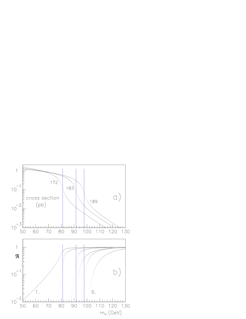
Figure 1: a) cross-section $e^{+}e^{-}\rightarrow H+Z^{\circ}$ as a function of $m_{H}$ for $\sqrt{s}=172,\,183,\,189$ GeV. The vertical lines are at $m_{H}=\sqrt{s}-M_{Z}$. b) ${\cal R}$ vs. $m_{H}$ for $n_{obs}=\lambda_{B}=0$ for $\sqrt{s}=172,\,183,\,189$ GeV, with $\epsilon=30\%$ and ${\cal L}=10,\,55,\,180\>{\rm pb}^{-1}$ per experiment, respectively. Odd lines are for a single experiment, even ones represent the combination of four.

In this non ideal situation we expect the step function of Eq. (21) to be replaced by a smooth curve which goes to zero for low masses and to 1 for $M_{H}\rightarrow M_{K_{eff}}$, where the experimental sensitivity is lost. In this case dir. in Eq. (20) stands, in principle, for all possible experimental observables and the function $f(\mbox{\it dir.}\,|\,m_{H})$ should be provided by the experiments. However the LEP collaboration results on the Higgs mass searches are usually presented in terms of confidence level $(C.L.)$ [10]. As discussed in section 6 this quantity does not have a simple connection to $f(\mbox{\it dir.}\,|\,m_{H})$. Given this situation we decided to model the likelihood in a way which seems compatible with the physics case.

First, all possible experimental observables can, in practice, be replaced by suitable combinations which depend on the Higgs mass. The simplest of these possible “summaries” of the data is the number of observed candidate events, which we will indicate by $n_{obs}$. The number of candidate events expected to be observed, on the other hand, is given by the sum of the Higgs events, indicated by $\lambda_{S}(m_{H})$, and the expected number of background events, $\lambda_{B}$, assumed here to be well known (see e.g. Ref.[6] for the natural extension when $\lambda_{B}$ is uncertain too). The mass dependence of the former is due to the mass dependence of cross section, branching ratio $(b.r.)$ and efficiency, and so it depends on the decay channel investigated. For simplicity, we discuss the case of a likelihood obtained considering the total number of observed candidate events in a single channel. This is given by

$$f(n_{obs}\,|\,m_{H},\lambda_{B})=\frac{e^{-(\lambda_{S}(m_{H})+\lambda_{B})}\cdot(\lambda_{S}(m_{H})+\lambda_{B})^{n_{obs}}}{n_{obs}!}\,,$$ (22)

since $n_{obs}$ is expected to be described by a Poisson distribution with parameter $\lambda=\lambda_{S}(m_{H})+\lambda_{B}$. In order to compare and combine the updating power provided by each piece of information easily, it is convenient to replace the likelihood by a function, ${\cal R}$, that goes to 1 where the experimental sensitivity is lost [11]. This function can be seen as the counterpart, in the case of a real experiment, of the step function of Eq. (21). Because constant factors do not play any role in the Bayes’ theorem we can divide the likelihood by its value calculated for very large Higgs mass values, where no signal is expected, i.e. $M_{H}\rightarrow\mbox{``}\infty\mbox{''}$, or $\lambda_{S}\rightarrow 0$. Clearly, this operation makes sense only if the likelihood is different from 0 for $M_{H}\rightarrow\mbox{``}\infty\mbox{''}$. This condition is satisfied for any $\lambda_{B}$ in case $n_{obs}\neq 0$, but when $n_{obs}=0$ only for $\lambda_{B}=0$. The case of $n_{obs}\neq 0$ with $\lambda_{B}=0$ leads to a clear discovery, i.e. the likelihood will assume positive values only below $M_{K_{eff}}$ and there is no need anymore to build the ${\cal R}$ function with the desired asymptotic properties.

${\cal R}$, as a mathematical function of $m_{H}$, with $n_{obs}$ and $\lambda_{B}$ acting as parameters, can be seen as a kind of shape distortion function of the p.d.f. introduced by the new data. As long as ${\cal R}(m_{H})$ is 1, the shape (and therefore the relative probabilities in that region) remains unchanged, while in the limit ${\cal R}(m_{H})\rightarrow 0$ the p.d.f. vanishes. One should notice that ${\cal R}(m_{H})$ can also assume values larger than 1 in the region of sensitivity, corresponding to a number of observed candidate events larger than the expected background. In this case the p.d.f. will be stretched below the effective kinematical limit and this might even prompt a claim for a discovery if ${\cal R}$ becomes sufficiently large for the probability of $M_{H}$ in that region to get very close to 1.

Applying this formalism to our case and in the realistic situation of non vanishing expected background we get

$${\cal R}(m_{H};n_{obs},\lambda_{B})=\frac{e^{-(\lambda_{S}(m_{H}))}\cdot(\lambda_{S}(m_{H})+\lambda_{B})^{n_{obs}}}{\lambda_{B}^{n_{obs}}}\,,~{}~{}(\lambda_{B}\neq 0,\>\mbox{if}~{}~{}n_{obs}\neq 0).$$ (23)

Instead, when $\lambda_{B}=0$ and $n_{obs}=0$ one can take the limit of the above formula obtaining ${\cal R}(m_{H})=e^{-\lambda_{S}(m_{H})}$. Examples of this function are shown in figure 1b) in case of no events candidates and zero background ($n_{obs}=\lambda_{B}=0$), for $\sqrt{s}=172,\,183$ and 189 GeV, considering a single LEP experiment (odd numbers) and the combination of all experiments (even numbers). The calculations have been done assuming a nominal integrated luminosity per experiment of 10, 55 and 180 pb^-1 for the three energies, and an average and constant detection efficiency of 30 %. Fig.2, instead, illustrates six different possible scenarios. In the figure we consider a search at $\sqrt{s}=183$ GeV with ${\cal L}=55\,{\rm pb}^{-1}$ by a single experiment that looks for two Higgs decay channels with different branching ratio. For each channel we plot 3 different situations of expected background and observed number of events.

Figure 2: ${\cal R}$ vs. $m_{H}$ for two search channels at $\sqrt{s}=183$ GeV with ${\cal L}=55\,{\rm pb}^{-1}$. The lines a–c represent a channel with $b.r.\times\epsilon=1.7\%$ while d–f correspond to a search with $b.r.\times\epsilon=32\%$. The cases considered are: $n_{obs}=2,\,\lambda_{B}=0.2\>\mbox{(a,\,d)};\>n_{obs}=3,\,\lambda_{B}=3\>\mbox{(b,\,e)};\>n_{obs}=0,\,\lambda_{B}=1.5\>\mbox{(c,\,f)}$.

As already pointed out, $f(\mbox{\it dir.}\,|\,m_{H})$, and hence ${\cal R}(m_{H};\mbox{\it dir.})$, might be more complicated than the simplified likelihood used here, and it can only be provided by experiments. Either of the above functions would be the most unbiased way of reporting the experimental result and it would allow several pieces of experimental information to be easily combined. In fact, when individual experiments or decay channels are independent the overall likelihood is simply the product of the individual likelihoods and therefore

$${\cal R}(m_{H};\mbox{``all data''})=\Pi_{i}{\cal R}_{i}(m_{H};\mbox{``data $i$''})\,,$$ (24)

and this can be used in Eq. (20) to get the distribution of $M_{H}$ which takes into account all available data.

4 Input quantities entering the indirect determination

In this section we discuss the experimental and theoretical inputs used in our analysis.

Hadronic contribution to QED vacuum polarization

The QED coupling at the $Z$ boson mass scale plays an important role in the prediction of $m_{H}$. This fact has always stimulated a lot of activity on the exact determination of $(\Delta\alpha)_{h}$. The most phenomenological analyses of it rely on the use of all the available experimental data on the hadron production in $e^{+}\,e^{-}$ annihilation and on perturbative QCD (pQCD) for the high energy tail ($E\geq 40$ GeV) of the dispersion integral. The reference value in this approach is [12]

$$(\Delta\alpha)_{h}^{EJ}=0.02804\pm 0.00065~{}.$$ (25)

In the recent past the hadronic contribution to the vacuum polarization has been the subject of several new investigations that advocate the use of pQCD down to energy scale of the order of 1 GeV [13, 14]. In this more theory driven path, the various analyses differ on the energy value at which to start applying pQCD and on the amount of theoretical inputs used to evaluate the experimental data in the regions, like, for example, the threshold for the charmed mesons, where pQCD is not applicable. The common characteristic of these works with respect to the most phenomenological ones is to obtain a smaller central value for $(\Delta\alpha)_{h}$ with a reduced uncertainty. The most stringent result of these theory oriented analyses is [14]

$$(\Delta\alpha)_{h}^{DH}=0.02763\pm 0.00016$$ (26)

that we will use in the sequel as reference value for this kind of approach.

At the moment there is no definite argument for choosing one or other of the two approaches. The results are absolutely compatible to each other. However, the numerical difference between central values and uncertainties is such that it prevents an easy estimation of the effect of choosing one value instead of the other. For these reasons we decided to present our results for the values of $(\Delta\alpha)_{h}$ given by $(\Delta\alpha)_{h}^{EJ}$ and $(\Delta\alpha)_{h}^{DH}$ separately.

Top quark mass

The value of the top quark used in our analysis is the combination of the experimental direct measurements reported by CDF [15] and D0 [16]:

$$M_{t}=174.2\pm 4.8~{}\mbox{GeV}.$$ (27)

The $M_{t}$ value obtained in the global fit of the EWWG [5], that uses as experimental value input $M_{t}=173.8\pm 5.0$ GeV, is actually a little bit smaller, i.e. $M_{t}=171.1\pm 4.9$ GeV. The principal cause for this smaller value is connected with the remnant of the famous $R_{b}$ “anomaly”. In our analysis we assume the validity of the SM and therefore we prefer to use the experimental result of Eq. (27).

QCD strong coupling constant

Among the various input quantities, the strong coupling constant at the $M_{Z}$ scale is the least important. In fact, QCD effects appear in the theoretical calculations of $s^{2}_{eff}$ and $M_{W}$ only at the two loop level. We use the world average [17]

$$\alpha_{s}(M_{Z})=0.119\pm 0.002$$ (28)

Effective mixing parameter $\sin^{2}\theta_{eff}^{lept}$

The effective Weinberg angle is the quantity that has the greatest sensitivity to the Higgs. Therefore its precise value is very important in determining $f(m_{H})$. There is overall good agreement among all the measurements although the two most precise ones, i.e. $A_{{\rm LR}}$ from SLD ($s^{2}_{eff}=0.23109\pm 0.00029$) and $A_{{\rm FB}}^{0,{\rm b}}$ from LEP ($s^{2}_{eff}=0.23225\pm 0.00038$), are still about two and a half standard deviations apart. However, the continual raising of the SLD value during the recent years together with some reduction of the $A_{{\rm FB}}^{0,{\rm b}}$ result has significantly improved the agreement between the average LEP and SLD determinations. In this situation we do not see any particular reason either for excluding the SLD values or for attributing to it a smaller weight [18]. Therefore we employ in our analysis the combined LEP+SLD average[5]

$$\sin^{2}\theta_{eff}^{lept}=0.23157\pm 0.00018.$$ (29)

$W$ boson mass

The present experimental information on $M_{W}$ comes from the invariant mass of its decay products (LEP and Tevatron), from the threshold behaviour of the production cross section (LEP) and from the electroweak coupling constant in neutrino scattering (NuTeV,CCFR). The first two measurements can be considered a kind of “direct” determinations of the mass, in the sense that they are sensitive directly to it and not to a combination of other parameters of the SM. The combination of CDF [19], D0 [20] and LEP values [5] (including also the old UA2 measurement [21]), gives[5]:

$$M_{W}^{k}=80.39\pm 0.06~{}\mbox{GeV}.$$ (30)

The result of the deep inelastic scattering experiments can be reported using the quantity $\sin^{2}\theta_{w}=1-M_{W}^{2}/M_{Z}^{2}$. In this case $M_{W}$ can be extracted in terms of the very precise $M_{Z}$ value plus top quark and Higgs boson mass corrections [22]:

$$\frac{M_{W}^{dis}}{\mbox{GeV}}=\frac{M_{W}^{\nu}}{\mbox{GeV}}+0.073\,\left(\frac{M_{t}^{2}-(175\,\mbox{GeV})^{2}}{(100\,\mbox{GeV})^{2}}\right)-0.025\,\ln(M_{H}/150\,\mbox{GeV})\,,$$ (31)

where $M_{W}^{\nu}$ indicates the result at the reference values ($M_{t}=175\,\mbox{GeV}$ and $M_{H}=150\,\mbox{GeV})$:

$$M_{W}^{\nu}=80.25\pm 0.11\,\mbox{GeV}\,.$$

In order to make use of all available information we proceed in the following way. We evaluate $A_{1}^{w}$ from $M_{W}^{k}$ and $M_{W}^{dis}$ separately using Eq. (2) (in the $M_{W}^{dis}$ case the Higgs and top dependence can be accounted for by redefining the theoretical coefficients $d_{1}$, $d_{3}$, and $M_{W}^{\circ}$). Once the compatibility of the two results has been established, we are allowed to combine directly the $M_{W}$ values weighting them with the inverse of the variance. We obtain

$$\frac{M_{W}}{\mbox{GeV}}=80.36\pm 0.05+0.0023-0.0057A_{1}+0.051A_{3}$$ (32)

which is the value employed in the analysis. Again, the Higgs and top dependence is taken into account by slightly modifying the relevant coefficients in Eq. (2).

Theoretical coefficients

The various coefficients entering Eqs. (1) and (2) are not known exactly due to truncation of the perturbative series. This uncertainty is usually estimated comparing the results of different schemes of calculation that contain all the available theoretical information at a given order of accuracy. Then the simplest procedure is to evaluate the best value and standard deviation associated to the uncertainty of each of the coefficients from the average and standard deviation of the values given in Ref.[4] (when all renormalization schemes yield the same numerical results the standard deviation is that due to the rounding, i.e. unit of the least significant digit divided by $\sqrt{12}$). They are indicated in tables 1, 2 and 3 and considered independent in the uncertainty propagation. Let us comment on the meaning and the use of averages and standard deviations for the coefficients. Taking as an example $c_{1}$, we get (in units $10^{-4}$) $\mbox{E}[c_{1}]=5.23$ and $\sigma(c_{1})=0.04$, obtained by the following numbers[4]: 5.23, 5.19 and 5.26. This does not imply that necessarily one has to believe that 5.23 is really more preferred than the others, as a Gaussian distribution centered in 5.23 with standard deviation 0.04 would imply. One could imagine a uniform distribution ranging between 5.16 and 5.30; or a triangular distribution centered in 5.23 and going to zero at 5.13 and 5.23; or any other distribution having mean 5.23 and sigma 0.04. The final result, relying on the central limit theorem, which, for the relative sizes of the standard deviations of interests ensures a fast convergence, will not depend on the shape of the particular distribution (they could also be different for different coefficients).

It should be noticed that the values presented in Ref.[4] do not cover uncertainties associated to QCD contribution in electroweak corrections. The dominant part of it is included in $\delta_{QCD}$, the relevant correction in the electroweak parameter $\Delta\rho$. The uncertainty in $\delta_{QCD}$ will reflect itself in a correlated way in the various theoretical coefficients.

To judge the effect of possible correlations in the values given in Ref.[4] we use the method outlined at the end of Sect. 2. The more rigorous results derived with this procedure are practically identical to those obtained using average values and standard deviations of each coefficient. This is shown in table 3 and 4 where the comparison of the two methods is presented. In the combined final $A_{1}$ result we report an additional digit to test the accuracy due to rounding. Also the final shape of the p.d.f. of $A_{1}$ obtainable from Eq. (9) is Gaussian with a good degree of approximation, since it is the average of three Gaussians (each of which is justified by the central limit theorem) and the closeness of their centers is much smaller than their widths. Given this situation, we present our result as a function of average coefficients and of their standard deviations, because this method shows the sensitivity of $A_{1}$ to the various parameters in a clear way.

5 Results from the indirect determination

The determinations of $M_{W}$ is presented in table 1. The two values reported are obtained for $(\Delta\alpha)_{h}^{EJ}$ ($M_{W}=80.375\pm 0.027$ GeV) and $(\Delta\alpha)_{h}^{DH}$ ($M_{W}=80.366\pm 0.025$ GeV). The two results are consistent and both are well in agreement with the experimental determinations given in (30) and (31). The uncertainty on the indirect $M_{W}$ determination is still a factor $\approx 2$ better than the present direct experimental result. The table also shows the contribution to the total uncertainty of each input quantity, with the sign of the derivative calculated in the reference point. This information allows the result to be corrected if any input quantity slightly changes in expected value or standard deviation. Through the entries in table 1 we can estimate the shift in the predicted central value due to unknown QCD effects in electroweak corrections. Indeed a variation in $\delta_{QCD}$ introduces a shift on the calculated $s^{2}_{eff}$ and $M_{W}$ of $\delta s^{2}_{eff}\approx-1\cdot 10^{-7}\,\delta(\delta_{QCD})\,M_{t}^{2}$ and $\delta M_{W}\approx 2\cdot 10^{-5}\,\delta(\delta_{QCD})\,M_{t}^{2}$ (GeV). For $M_{t}=175$ GeV, $\delta(\delta_{QCD})$ has been estimated $\approx 5.2\cdot 10^{-3}$ [23]. This induces shifts in the values of $s^{2}_{eff}$ and $M_{W}$ that amount to $-1.8\cdot 10^{-5}$ and $3.1$ MeV respectively. Using table 1 one finds an additional uncertainty in the predicted $M_{W}$ central value, $\delta M_{W}\approx 1$ MeV.

The determination of $M_{H}$ from the effective mixing angle and $M_{W}$ separately is presented in table 2 ($(\Delta\alpha)_{h}=(\Delta\alpha)_{h}^{EJ}$) and table 3 ($(\Delta\alpha)_{h}=(\Delta\alpha)_{h}^{DH}$). All values are given in TeV to reduce the number of digits to the significant ones. The table also shows the combined determination. The values of $A_{1}^{s}$ and $A_{1}^{w}$ are in agreement within uncertainty. However, the $M_{W}$ determination is much less precise and the effect of combining it with $A_{1}^{s}$ has almost a negligible impact on the determination of the Higgs mass from $s^{2}_{eff}$, also because of the correlation between them. In case of slight variation of the central values of the input quantities the $A_{1}$ result can be corrected using the information provided in the tables. However the same procedure cannot be applied in case of changes of the standard deviations because $A_{1}$ is obtained through a combination where the inverse of variances enters. For the same reason input quantities with large uncertainty are dumped in the combination and therefore they give a small contribution to the total $A_{1}$ uncertainty. In the various tables, combination results are indicated by “$\ast$” below the relevant column.

Among the various observables whose theoretical prediction depend upon $M_{H}$, given the present values of the $A_{2}$–$A_{4}$ quantities, $s^{2}_{eff}$ is by far the most effective in constraining $M_{H}$. Any other, like e.g. $M_{W}$ or the leptonic width, has a very modest weight in a combined analysis. This fact justifies our choice of considering only one observable, $M_{W}$, in addition to $s^{2}_{eff}$. This situation will not change in the near future. In fact, a $W$ mass as effective in the $M_{H}$ indirect determination as the present $s^{2}_{eff}$ requires not only a very precise $M_{W}$ result ($\sigma(M_{W})\leq 25$ MeV) but also a reduction in $M_{t}$ uncertainty ($\sigma(M_{t})\leq 2.5$ GeV), as already pointed out in Ref.[24].

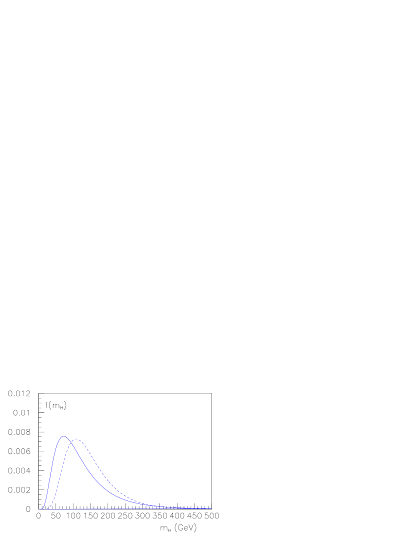
Figure 3: Probability distribution function for the Higgs mass from precision measurements. The solid line is obtained employing $(\Delta\alpha)_{h}=0.02804\pm 0.00065$, the dashed one with $(\Delta\alpha)_{h}=0.02763\pm 0.00016$

Figure 3 presents the p.d.f. of $M_{H}$ obtained using only the indirect information. The comparison of the two curves shows that the use of a higher central value for $(\Delta\alpha)_{h}$ (i.e. $(\Delta\alpha)_{h}^{EJ}$) tends to concentrate more the probability towards smaller values of $M_{H}$. This can be understood from the negative derivative of $M_{H}$ with respect to $(\Delta\alpha)_{h}$, shown in tables 2 and 3. Indeed, in this case the median of the distribution is $M^{50}_{H}=0.10$ TeV while the analysis performed employing $(\Delta\alpha)_{h}^{DH}$ gives for the same quantity a result $\approx 0.3$ TeV higher, which is still less than half a standard deviation of the distribution. It is interesting to note that although the $A_{1}$ expected values and standard deviations in table 2 and 3 are different, they actually give very close 95 % probability upper limit, $M_{H}^{95}$. Similarly, while $(\Delta\alpha)_{h}^{DH}$ has an uncertainty that is approximately $4$ times smaller than $(\Delta\alpha)_{h}^{EJ}$, the standard deviations of the two $M_{H}$ p.d.f.’s are very close too. Finally, we note that a variation in $\delta_{QCD}$ of the order of magnitude discussed above increases $M_{H}^{95}$ by $\approx 10$ GeV.

6 Results including the direct search

An extensive program to look for evidence of Higgs production in $e^{+}e^{-}$ collision has been pursued at LEP during the last decade. Presently results for Higgs searches by all four LEP collaborations are available for center of mass energies up to $\sqrt{s}=183$ GeV [25, 26, 27, 28]. The negative outcome of these searches has been reported as a combined 89.8 GeV “$95\,\%\,C.L.$” lower bound [29, 30]. Unfortunately this result has no simple probabilistic interpretation regarding the Higgs mass [31]. The operational definition of the limit is expressed in terms of a test-statistic, $X$, based on the number of selected events and their distribution in a variable that discriminates signal from background, whose value measured in the data, $X_{obs}$, is compared to that obtained on the basis of a large number of “simulated gedanken experiments” [10], or

$$CL_{s}(m_{H})=\frac{CL_{s+b}(m_{H})}{CL_{b}(m_{H})}=\frac{P(X_{s+b}(m_{H})\leq X_{obs})}{P(X_{b}(m_{H})\leq X_{obs})}~{}~{}.$$ (33)

The $C.L.$ for the signal + background hypothesis, $CL_{s+b}$, is defined as the probability that the test-statistic is less than or equal to $X_{obs}$, where the p.d.f of $X_{s+b}$ is obtained by the Monte Carlo generation of experiments in which a signal with mass $m_{H}$ is introduced in addition to the background. The corresponding $C.L.$ for the signal, $CL_{s}$, is then obtained by normalizing $CL_{s+b}$ to $CL_{b}$, the $C.L.$ for the background only hypothesis, where the p.d.f. of $X_{b}$ is obtained similarly to that of $X_{s+b}$ but generating experiments with no signal. One can realize that the $C.L.$ curves do not correspond to the likelihood of the observed data as a function of the Higgs mass (i.e. $f(\mbox{\it dir.}\,|\,m_{H})$). Therefore, the published combined limit cannot be translated into a number which could be used in an unambiguous way in our analysis.

As outlined in section 3, the information from the direct search could easily be incorporated into the analysis if we had the likelihood or, more simply, the ${\cal R}$ function. We note here that the test-statistic $X_{obs}$ of method A of Ref.[10] actually corresponds to ${\cal R}$. The publication of its value as a function of $m_{H}$ would be sufficient for a complete analysis to be performed. However, at the moment, this information is not available.

Although we are not in a position to make a detailed analysis, we can estimate the effect of the direct search results on the final p.d.f. of $m_{H}$ by employing the simplified likelihood given in Eq. (22) and the public values of observed number of events, expected backgrounds and efficiencies. With respect to this a few remarks are in order: i) in the function ${\cal R}$ the important effect is always given by the data at the last energy point available. In fact, because the final likelihood of searches at different energies is given by the product of the individual likelihoods at the various $\sqrt{s}$, in the region of $M_{H}$ values close to $M_{K_{eff}}$ of the highest energy point, the region which we are interested in, only the corresponding ${\cal R}$ will be relevant because those of lower energies are already saturated to 1. In our study we thus only use data at $\sqrt{s}=183$ GeV [25, 26, 27, 28]. ii) Differently from the other three experiments, L3 uses selection criteria that depend on $m_{H}$. Correspondingly the number of selected events and backgrounds will be functions of $m_{H}$. This situation is not compatible with our simplified likelihood. Therefore we do not consider the L3 data. iii) Eq. (22) does not contain any information related to the distribution of the signal and the backgrounds. At the level at which we can perform our analysis using only public results, shape effects cannot be taken into account. However, the observed number of events in the various channels reported by the three collaborations are always either zero or few units. Given this situation we expect that it is the event counting which gives most of the constraint.

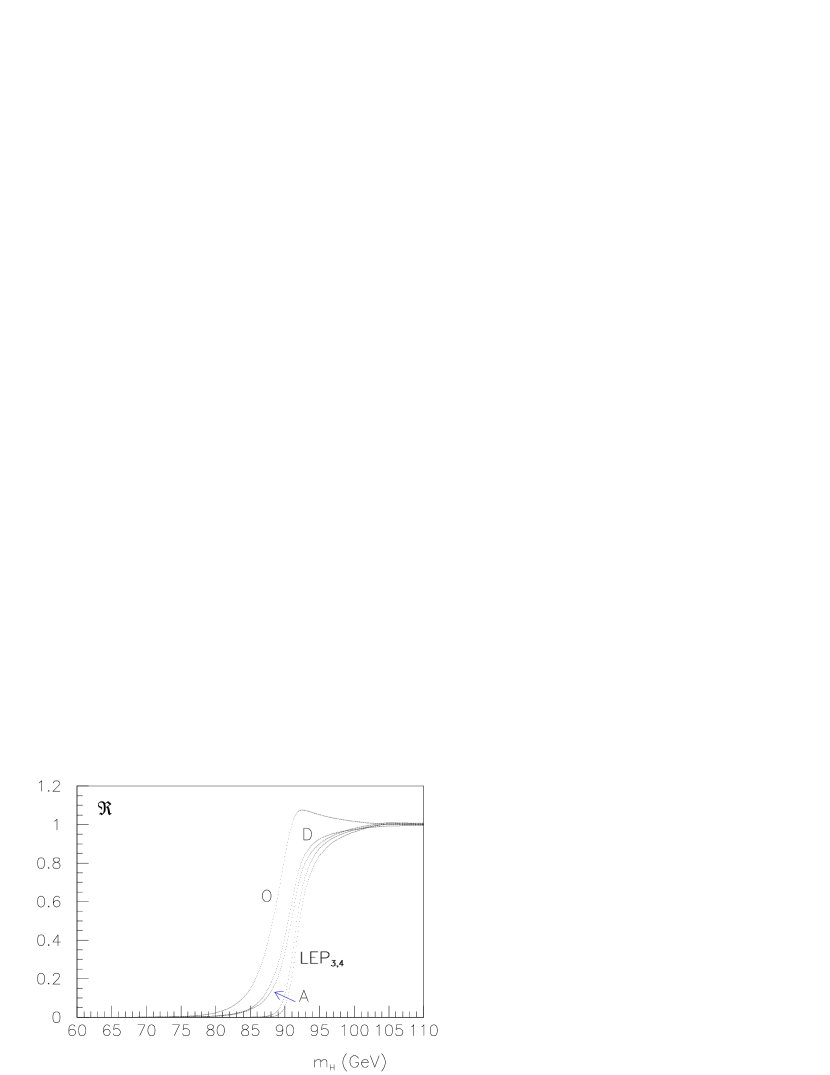
Figure 4: ${\cal R}$ vs. $m_{H}$ for the search at $\sqrt{s}=183$ GeV. The curves A, D, O correspond to the single experiment. The ${\rm LEP}_{3}$ line represents the combination of the three. The curve ${\rm LEP}_{4}$ is obtained by raising the ${\rm LEP}_{3}$ one to the $4/3$ power.

Figure 4 presents the ${\cal R}$ curves for the three experiments, ALEPH (A), DELPHI (D) and OPAL (O). Each curve is obtained by multiplying the ${\cal R}$’s of the individual search channels of the experiment. The overall ${\cal R}$ for the combination of three experiments is also shown labeled as ${\rm LEP}_{3}$. As already said, we cannot use L3 data. To try to take into account the L3 contribution we make the assumption that the L3 results are on average similar to those of the other experiments. We then roughly estimate the effect of L3, simply raising the combined ${\cal R}$ of the other three experiments to the $4/3$ power. The corresponding curve is presented in Fig. 4 marked ${\rm LEP}_{4}$. We note that the OPAL ${\cal R}$ curve presents a bump which is connected to a small excess of the observed number of events with respect to the expected background in the $q\bar{q}H$ channel. This bump is not particularly significant for two reasons: i) it is not very pronounced and therefore when the OPAL ${\cal R}$ is combined with $f(m_{H}\,|\,\mbox{\it ind.})$ the probability in the corresponding Higgs mass region is not particularly enhanced. ii) Our analysis is based on the event counting only and ignores the distribution of the signal and background. When the latter information is also taken into account it is not unlikely that this bump disappears.

According to Eq. (20) the final p.d.f. is obtained by combining the p.d.f. coming from precision measurements (Fig. 3) with the likelihood derived from the LEP data (Fig. 4), rescaled to the function ${\cal R}$, or

$$f(m_{H}\,|\,\mbox{\it dir.}\,\&\,\mbox{\it ind.})=\frac{{\cal R}(m_{H})\,f(m_{H}\,|\,\mbox{\it ind.})}{\int_{0}^{\infty}{\cal R}(m_{H})\,f(m_{H}\,|\,\mbox{\it ind.})\,dm_{H}}~{}.$$ (34)

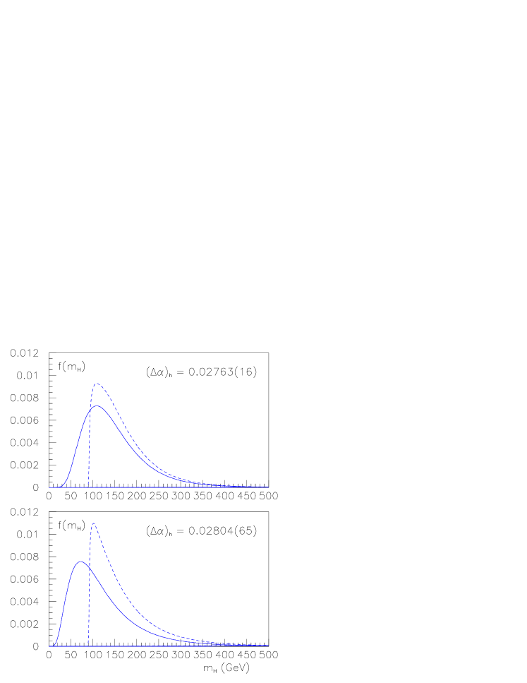
Figure 5: Probability distribution functions using only indirect information (solid line) and employing also the experimental results from direct searches (dashed one).

The result is shown in figure 5 where $f(m_{H}\,|\,\mbox{\it dir.}\,\&\,\mbox{\it ind.})$ is compared to $f(m_{H}\,|\,\mbox{\it ind.})$ for each assumption on $(\Delta\alpha)_{h}$. To judge the sensitivity of $f(m_{H}\,|\,\mbox{\it dir.}\,\&\,\mbox{\it ind.})$ to the likelihood we have actually evaluated Eq. (34) using two different ${\cal R}$’s (${\rm LEP}_{3}$ and ${\rm LEP}_{4}$). The two resulting curves are indistinguishable as could be expected given that the two ${\cal R}$’s differ practically by a shift of $\approx 1/2$ GeV. To envisage a more different case, we compare the final distribution presented in fig. 5 with that we obtain in our simplified analysis using only OPAL data. The difference in the expected value amounts to 4-5 GeV, depending on the value of $(\Delta\alpha)_{h}$ chosen, while standard deviations are the same. The “OPAL” $M_{H}^{95}$ is 3-6 GeV lower than the one reported in table 5 where our final results are presented. The closeness of the various quantities shows that our results do not depend critically upon the details of the analysis.

As expected, the inclusion of the direct search information in the Higgs mass probability analysis drifts the p.d.f. towards higher values of $M_{H}$, changing its shape such that the probability of $M_{H}$ values below 95 GeV drops to $\approx 3\,\%$. Table 5 summarizes our analysis in terms of various convenient parameters of the distribution. Expected value, standard deviation, mode and median are not very sensitive to the values of the hadronic contribution to the vacuum polarization. Also in both cases, $75\,\%$ of the probability is concentrated in the region $M_{H}<0.20$ TeV. Instead the choice of $(\Delta\alpha)_{h}$ affects the tail of the distribution with $(\Delta\alpha)_{h}^{EJ}$ producing a longer one. Indeed while the use of only indirect information gives same values of $M_{H}^{95}$, when the direct one is also included, the $M_{H}^{95}$ obtained using $(\Delta\alpha)_{h}^{EJ}$ is $\sim 0.3$ TeV higher than the corresponding number for $(\Delta\alpha)_{h}^{DH}$, and this effect is even more pronounced for $M_{H}^{99}$.

7 Conclusions

We have presented a method that allows the Higgs mass to be constrained combining together the indirect information coming from precision measurements and accurate calculations, with the results of the search experiments currently being carried out at LEP. The method makes use of the Bayes’ theorem which allows the p.d.f. obtained from precision measurements to be augmented with the direct experimental information through the likelihoods of the various search channels. Such likelihoods should be provided by the experiments, possibly in the form of the ${\cal R}$ function that is very convenient for comparing and combining the various informations and it has also an intuitive interpretation because of its limit to the step function of the ideal case. Using the simplified form of Eq. (22) and the public results concerning observed number of events, backgrounds and efficiencies of the ALEPH, DELPHI, OPAL experiments for $\sqrt{s}=183$ GeV, we have derived a p.d.f. for the Higgs boson mass that includes the direct search constraint. Several parameters of the distribution has been reported and we have verified that the main conclusions do not depend to any great degree upon the detailed form of the likelihood.

It should be clearly stated that our results are derived under the assumption of the validity of the SM and using as input quantities those described in section 4. Our analysis does not apply to different frameworks, like for example the Minimal Supersymmetric Standard Model except the case when all SUSY particles are decoupled. Concerning the input quantities, our results depend largely upon the experimental value for $s^{2}_{eff}$ we have taken (Eq. (29)). It seems to us reasonable to employ the combined LEP+SLD value although, given the less than perfect agreement between the two most precise determinations, the suspicion that some measurements are affected by not yet understood systematic errors exists.

The last run of the LEP machine was performed at $\sqrt{s}=189$ GeV. Results on Higgs searches at this energy are still preliminary and only DELPHI has presented a somewhat detailed analysis of the searches in the $H+Z^{\circ}$ channel [32]. In the case of negative results by the other collaborations similar to those reported by DELPHI, we can make a rough estimation of the output of the search at $\sqrt{s}=189$ GeV by saying that the ${\cal R}$ will move 5-6 GeV towards higher values of $M_{H}$. The final $f(m_{H}\,|\,\mbox{\it dir.}\,\&\,\mbox{\it ind.})$ will be correspondingly shifted in the same direction.

We wish to thank F. Di Lodovico, R. Faccini and G. Ganis for useful communications and discussions.

$X_{i}$	E[$X_{i}$]	$\sigma(X_{i})$	$\frac{\partial M_{W}}{\partial X_{i}}\cdot\sigma(X_{i})$
			(MeV)
			$(\Delta\alpha)_{h}^{EJ}$	$(\Delta\alpha)_{h}^{DH}$
$(s^{2}_{eff})_{\circ}$	0.231525	0.000015	$+1.7$	$+1.8$
$c_{1}$	(5.23	0.04)$\cdot 10^{-4}$	$+1.8\cdot 10^{-3}$	$+0.13$
$c_{2}$	(9.860	0.003)$\cdot 10^{-3}$	$+4.7\cdot 10^{-4}$	$-4.7\cdot 10^{-3}$
$c_{3}$	(2.74	0.06) $\cdot 10^{-3}$	$+6.1\cdot 10^{-2}$	$+6.5\cdot 10^{-2}$
$c_{4}$	(4.47	0.06) $\cdot 10^{-4}$	$+5.6\cdot 10^{-3}$	$+6.1\cdot 10^{-3}$
$M^{\circ}_{W}$/GeV	80.3813	0.0012	$+1.2$	$+1.2$
$d_{1}$	0.0578	0.0004	$-1.6\cdot 10^{-3}$	$-0.11$
$d_{2}$	0.5177	0.0006	$-8.6\cdot 10^{-4}$	$+7.9\cdot 10^{-3}$
$d_{3}$	0.540	0.003	$-2.7\cdot 10^{-2}$	$-2.7\cdot 10^{-2}$
$d_{4}$	0.0850	0.0003	$-2.5\cdot 10^{-3}$	$-2.5\cdot 10^{-3}$
$d_{5}$	0.00793	0.00012	$-2.0\cdot 10^{-6}$	$-9.4\cdot 10^{-3}$
$(\Delta\alpha)_{h}$	0.02804	0.00065	$+13$
$(\Delta\alpha)_{h}$	0.02763	0.00016		$+3.7$
$M_{t}$/GeV	174.2	4.8	$+13$	$+12$
$\alpha_{s}(M_{Z})$	0.119	0.002	$-0.60$	$-0.54$
$s^{2}_{eff}$	0.23157	0.00018	$-20$	$-21$
$M_{W}$/GeV	80.375	0.027	$\leftarrow$
$M_{W}$/GeV	80.366	0.025		$\leftarrow$

Table 1: $M_{W}$ determination.

$X_{i}$	E[$X_{i}$]	$\sigma(X_{i})$	$\frac{\partial A_{1}}{\partial X_{i}}\cdot\sigma(X_{i})$
			“$s^{2}_{eff}$”	“$M_{W}$”	Comb.
$(s^{2}_{eff})_{\circ}$	0.231525	0.000015	$-0.029$		$-0.024$
$c_{1}$	(5.23	0.04)$\cdot 10^{-4}$	$-3.1\cdot 10^{-5}$		$-1.0\cdot 10^{-3}$
$c_{2}$	(9.860	0.003)$\cdot 10^{-3}$	$-8.2\cdot 10^{-6}$		$+1.3\cdot 10^{-5}$
$c_{3}$	(2.74	0.06)$\cdot 10^{-3}$	$-1.0\cdot 10^{-3}$		$-6.3\cdot 10^{-4}$
$c_{4}$	(4.47	0.06)$\cdot 10^{-4}$	$-9.7\cdot 10^{-5}$		$-8.2\cdot 10^{-5}$
$M^{\circ}_{W}$/GeV	80.3813	0.0012		$+0.021$	$+4.0\cdot 10^{-3}$
$d_{1}$	0.0578	0.0004		$-2.0\cdot 10^{-3}$	$+5.4\cdot 10^{-4}$
$d_{2}$	0.5177	0.0006		$-1.5\cdot 10^{-5}$	$-2.6\cdot 10^{-5}$
$d_{3}$	0.540	0.003		$-4.8\cdot 10^{-4}$	$-3.5\cdot 10^{-4}$
$d_{4}$	0.0850	0.0003		$-4.5\cdot 10^{-5}$	$-8.9\cdot 10^{-6}$
$d_{5}$	0.00793	0.00012		$-1.7\cdot 10^{-4}$	$+1.2\cdot 10^{-4}$
$(\Delta\alpha)_{h}$	0.02804	0.00065	$-0.44$	$-0.21$	$-0.41$
$M_{t}$/GeV	174.2	4.8	$+0.29$	$+0.47$	$+0.33$
$\alpha_{s}(M_{Z})$	0.119	0.002	$-0.014$	$-0.026$	$-0.017$
$s^{2}_{eff}$	0.23157	0.00018	$+0.34$		$+0.29$
$M_{W}^{k}$/GeV	80.39	0.06		$-0.82$	$-0.15$
$M_{W}^{\nu}$/GeV	80.25	0.11		$-0.45$	$-0.080$
				$\ast$	$\ast$
$A^{s}_{1}$	$0.00$	$\rightarrow$	0.63
$A_{1}^{w}$	$+0.28$	$\rightarrow$		1.07
			$\underbrace{\hskip 99.58464pt}_{\rho=+0.34}$
$A_{1}$	0.05	$\rightarrow$	0.61		$\leftarrow$
$M_{H}$/TeV	0.13	0.08	$\left(\hat{M}_{H}=0.07\,\mbox{TeV},\ M^{50}_{H}=0.10\,\mbox{TeV}\right)$

Table 2: Summary of indirect information. $A_{1}\equiv\ln(M_{H}/100\,\mbox{GeV})$, $(\Delta\alpha)_{h}=(\Delta\alpha)_{h}^{EJ}$. See text for the meaning of “$\ast$”.

$X_{i}$	E[$X_{i}$]	$\sigma(X_{i})$	$\frac{\partial A_{1}}{\partial X_{i}}\cdot\sigma(X_{i})$
			“$s^{2}_{eff}$”	“$M_{W}$”	Comb.
$(s^{2}_{eff})_{\circ}$	0.231525	0.000015	$-0.029$		$-0.026$
$c_{1}$	(5.23	0.04)$\cdot 10^{-4}$	$-2.1\cdot 10^{-3}$		$-2.3\cdot 10^{-3}$
$c_{2}$	(9.860	0.003)$\cdot 10^{-3}$	$+7.6\cdot 10^{-5}$		$+7.0\cdot 10^{-5}$
$c_{3}$	(2.74	0.06)$\cdot 10^{-3}$	$-1.0\cdot 10^{-3}$		$-8.4\cdot 10^{-4}$
$c_{4}$	(4.47	0.06)$\cdot 10^{-4}$	$-9.7\cdot 10^{-5}$		$-8.9\cdot 10^{-5}$
$M^{\circ}_{W}$/GeV	80.3813	0.0012		$+0.020$	$+1.8\cdot 10^{-3}$
$d_{1}$	0.0578	0.0004		$-2.8\cdot 10^{-3}$	$+5.0\cdot 10^{-6}$
$d_{2}$	0.5177	0.0006		$+1.4\cdot 10^{-4}$	$+1.1\cdot 10^{-5}$
$d_{3}$	0.540	0.003		$-4.7\cdot 10^{-4}$	$-1.6\cdot 10^{-4}$
$d_{4}$	0.0850	0.0003		$-4.3\cdot 10^{-5}$	$-4.1\cdot 10^{-6}$
$d_{5}$	0.00793	0.00012		$-3.5\cdot 10^{-4}$	$+3.2\cdot 10^{-5}$
$(\Delta\alpha)_{h}$	0.02763	0.00016	$-0.11$	$-0.050$	$-0.10$
$M_{t}$/GeV	174.2	4.8	$+0.29$	$+0.46$	$+0.30$
$\alpha_{s}(M_{Z})$	0.119	0.002	$-0.014$	$-0.025$	$-0.016$
$s^{2}_{eff}$	0.23157	0.00018	$+0.34$		$+0.32$
$M_{W}^{k}$/GeV	80.39	0.06		$-0.79$	$-0.071$
$M_{W}^{\nu}$/GeV	80.25	0.11		$-0.43$	$-0.039$
				$\ast$	$\ast$
$A^{s}_{1}$	0.28	$\rightarrow$	0.46
$A_{1}^{w}$	0.41	$\rightarrow$		1.01
			$\underbrace{\hskip 99.58464pt}_{\rho=+0.29}$
$A_{1}$	$\mathbf{0.29_{1}}$	$\rightarrow$	$\mathbf{0.45_{5}}$		$\leftarrow$
$M_{H}$/TeV	0.15	0.07	$\left(\hat{M}_{H}=0.11\,\mbox{TeV},\ M^{50}_{H}=0.13\,\mbox{TeV}\right)$

Table 3: Like table 2 but for $(\Delta\alpha)_{h}=(\Delta\alpha)_{h}^{DH}$.

$X_{i}$	E($X_{i}$)	$\sigma(X_{i})$	$\frac{\partial A_{1}}{\partial X_{i}}\cdot\sigma(X_{i})$
			“$\overline{\mbox{MS}}$”	“OSI”	“OSII”
$(\Delta\alpha)_{h}$	0.02763	0.00016	$-0.10$	$-0.10$	$-0.10$
$M_{t}$/GeV	174.2	4.8	$+0.31$	$+0.31$	$+0.30$
$\alpha_{s}(M_{Z})$	0.119	0.002	$-0.016$	$-0.016$	$-0.015$
$s^{2}_{eff}$	0.23157	0.00018	$+0.32$	$+0.32$	$+0.32$
$M_{W}^{k}$/GeV	80.39	0.06	$-0.072$	$-0.070$	$-0.070$
$M_{W}^{\nu}$/GeV	80.25	0.11	$-0.039$	$-0.038$	$-0.038$
			$\ast$	$\ast$	$\ast$
$A_{1}\,|\,R_{1}$ ($\overline{\mbox{MS}}$)	0.318	$\rightarrow$	0.456
$A_{1}\,|\,R_{2}$ (OSI)	0.293	$\rightarrow$		0.460
$A_{1}\,|\,R_{3}$ (OSII)	0.262	$\rightarrow$			0.448
			$\underbrace{\hskip 142.26378pt}_{\sigma^{2}(A_{1})=\frac{1}{3}\sum_{i}\sigma^{2}(A_{1}\,|\,R_{i})+\sigma_{E}^{2}}$
$A_{1}$ (average)	$\mathbf{0.29_{1}}$	$\rightarrow$	$\mathbf{0.45_{5}}$

Table 4: Renormalization scheme dependence. The results shown here should be compared with those of table 3.

	$(\Delta\alpha)_{h}=0.02804(65)$		$(\Delta\alpha)_{h}=0.02763(16)$
	$(ind.)$	$\left(\begin{array}[]{c}ind.\\ +\\ dir.\end{array}\right)$	$(ind.)$	$\left(\begin{array}[]{c}ind.\\ +\\ dir.\end{array}\right)$
$\mbox{\bf E}[\mathbf{M_{H}}]$/TeV	0.13	0.17	0.15	0.17
$\mathbf{\sigma(M_{H})}$/TeV	0.08	0.08	0.07	0.07
$\hat{M}_{H}$/TeV	0.07	0.10	0.11	0.11
$\mathbf{M^{50}_{H}}$/TeV	0.10	0.15	0.13	0.15
$P(M_{H}\leq 95\,\mbox{GeV})$	44 %	3.2 %	23 %	2.3 %
$P(M_{H}\leq 0.11\,\mbox{TeV})$	53 %	19 %	33 %	16 %
$P(M_{H}\leq 0.13\,\mbox{TeV})$	64 %	38 %	48 %	34 %
$P(M_{H}\leq 0.20\,\mbox{TeV})$	86 %	75 %	81 %	76 %
$\mathbf{M^{95}_{H}}$/TeV; $P(M_{H}\leq M^{95}_{H})\approx 0.95$	0.28	0.33	0.28	0.30
$\mathbf{M^{99}_{H}}$/TeV; $P(M_{H}\leq M^{99}_{H})\approx 0.99$	0.43	0.48	0.39	0.40
$\left\{\!\!\begin{array}[]{l}M_{1}/\mbox{TeV};\ P(M_{H}<M_{1})\approx 0.16\\ M_{2}/\mbox{TeV};\ P(M_{H}>M_{2})\approx 0.16\end{array}\right.$	$\left\{\!\!\begin{array}[]{l}0.06\\ 0.19\end{array}\right.$	$\left\{\!\!\begin{array}[]{l}0.11\\ 0.23\end{array}\right.$	$\left\{\!\!\begin{array}[]{l}0.08\\ 0.21\end{array}\right.$	$\left\{\!\!\begin{array}[]{l}0.11\\ 0.23\end{array}\right.$
$\left\{\!\!\begin{array}[]{l}\mathbf{M_{3}}/\mbox{TeV};\ P(M_{H}<M_{3})\approx 0.25\\ \mathbf{M_{4}}/\mbox{TeV};\ P(M_{H}>M_{4})\approx 0.25\end{array}\right.$	$\left\{\!\!\begin{array}[]{l}0.07\\ 0.16\end{array}\right.$	$\left\{\!\!\begin{array}[]{l}\mbox{\bf 0.12}\\ \mbox{\bf 0.20}\end{array}\right.$	$\left\{\!\!\begin{array}[]{l}0.10\\ 0.18\end{array}\right.$	$\left\{\!\!\begin{array}[]{l}\mbox{\bf 0.12}\\ \mbox{\bf 0.20}\end{array}\right.$

Table 5: Summary of the direct plus indirect information.

References

- [1] see, e.g., G. Altarelli, R. Barbieri and F. Caravaglios, Int. J. Mod. Phys. A13 (1998) 1031., and references therein.
- [2] G. Degrassi, P. Gambino, and A. Sirlin, Phys. Lett. B394 (1997) 188.
- [3] G. Degrassi, P. Gambino, and A. Vicini, Phys. Lett. B383 (1996) 219.
- [4] G. Degrassi, P. Gambino, M. Passera and A. Sirlin, Phys. Lett. B418, (1998) 209.
- [5] G. Quast, Report of the LEP Electroweak Working Group to LEP Experiments Committee Meeting, CERN-Geneva, Sept. 15th 1998.
- [6] G. D’Agostini, “Probabilistic reasoning in HEP - principles and applications”, CERN Yellow Report in preparation.
- [7] G. D’Agostini, Nucl. Instr. Meth. A346 (1994) 306.
- [8] G. Cowen, “Statistical data analysis”, Oxford University Press, 1998.
- [9] N.L. Johnson and S. Kotz, “Distributions in statistics”, Houghton Mifflin, 1970.
- [10] ALEPH, DELPHI, L3 and OPAL Collaborations, The LEP working group for Higgs boson searches, CERN-EP/98-046, April 1, 1998 and references therein.
- [11] G. D’Agostini, ZEUS-Note-98-079, November 1998, paper in preparation.
- [12] S. Eidelman, F. Jegerlehner, Z. Phys. C67 (1995) 585; H. Burkhardt, B. Pietrzyk, Phys. Lett. B356 (1995) 398.
- [13] A.D. Martin and D. Zeppenfeld, Phys. Lett. B345 (1994) 558; M. Davier and A. Höcker, Phys. Lett. B419 (1998) 419; J.H. Kühn and M. Steinhauser, Phys. Lett. B437 (1998) 425; S. Groote, J.G. Körner, K. Schilcher and N.F. Nasrallah, Phys. Lett. B440 (1998) 375; J. Erler, preprint UPR-796T, hep-ph/9803453.
- [14] M. Davier and A. Höcker, Phys. Lett. B435 (1998) 427.
- [15] F.Abe et al. (CDF Collaboration), Phys. Rev. Lett. 82, (1999) 271.
- [16] B. Abbot et al. (D0 Collaboration), FERMILAB-PUB-98/261-E, hep-ex/9808029.
- [17] The Particle Data Group, C. Caso et al., Euro. Phys. Journal C3, (1998) 1.
- [18] M.S. Chanowitz, preprint LBNL-42103, hep-ph/9807452.
- [19] T. Dorigo (for the CDF Collaboration), FERMILAB-CONF-98/239-E, March 1998.
- [20] B. Abbot et al. (D0 Collaboration), Phys. Rev. Lett. 80, (1998) 3008.
- [21] J. Alitti et al. (UA2 Collaboration), Phys. Lett. B276 (1992) 354.
- [22] J. Yu (for the NuTev, D0 and CDF Collaborations), hep-ex/9806032.
- [23] K. Philippides and A. Sirlin, Nucl.Phys. B450 (1995) 3 and Refs. cited therein. P. Gambino and A. Sirlin, Phys. Lett. B355 (1995) 295.
- [24] G. Degrassi, Acta Phys. Pol. B29 (1998) 2683.
- [25] R. Barate et al. (ALEPH Collaboration), Phys. Lett. B440 (1998) 403.
- [26] DELPHI98-95 CONF 163, conference submission ICHEP’98-200.
- [27] H. Acciari et al. (L3 Collaboration), Phys. Lett. B431 (1998) 437.
- [28] G. Abbiendi et al. (OPAL Collaboration), CERN-EP/98-173, hep-ex/9811025, to be published in the European Physics Journal C.
- [29] LEP Higgs Working Group, ALEPH 98-069 PHYSIC 98-028, DELPHI 98-144 PHYS 790, L3 Note 2310, OPAL Thecnical Note TN-588, July 1998.
- [30] F. Di Lodovico, Report of the LEP Higgs Working Group to LEP Experiments Committee Meeting, CERN-Geneva, Sept. 15th 1998.
- [31] G. D’Agostini, physics/9811046.
- [32] V. Ruhlmann-Kleider, Report to LEP Experiments Committee Meeting, CERN-Geneva, Nov. 12th 1998.