Was the Electroweak Phase Transition
Preceded by a Color-Broken Phase?

Abstract

It has been suggested, in connection with electroweak baryogenesis in the Minimal Supersymmetric Standard Model (MSSM), that the right-handed top squark has a negative mass squared parameter, such that its field could condense prior to the electroweak phase transition (EWPT). Thus color and electric charge could have been broken just before the EWPT. Here we investigate whether the tunneling rate from the color-broken vacuum can ever be large enough for the EWPT to occur in this case. We find that, even when all parameters are adjusted to their most favorable values, the nucleation rate is many orders of magnitude too small. We conclude that, without additional physics beyond the MSSM, the answer to our title question is “no.” This gives constraints in the plane of the light stop mass versus parameters related to stop mixing. However it may be possible to get color breaking in extended models, such as those with $R$-parity violation.

MCGILL-99/01

hep-ph/9902220

1 Introduction

The baryon asymmetry of the universe (the excess of baryons over antibaryons) is a very interesting puzzle, and it is exciting that its resolution may involve only electroweak physics which is either known or testable at colliders in the near future. This is because electroweak physics has the potential for satisfying all three of Sakharov’s conditions [1] for baryogenesis. The first, baryon number nonconservation, occurs because of the anomaly and the topological structure of the vacuum in the SU(2) sector of the electroweak theory [2]; further, baryon number violation becomes quite efficient at high temperatures, $T>100$ GeV [3]. The second condition, CP violation, is present but insufficient in the minimal standard model [4]; however, there are new sources in some extended models which allow for enough baryon production.

The third condition is that baryon number violating processes are out of thermal equilibrium, at the moment of baryogenesis. Electroweak physics can assure this as temperatures fall through the $T\sim 100$ GeV range if the Higgs field gains a large condensate at a first order phase transition. To avoid the relaxation of baryon number back to zero in the broken phase, the Higgs condensate $h$ must satisfy $h/T\mbox{\raisebox{-2.58334pt}{~{}$\stackrel{{\scriptstyle>}}{{\scriptscriptstyle\sim}}$~{}}}1.1$ [5]. Such a strong phase transition is not guaranteed, but it depends on the exact values of masses and couplings. In the standard model it does not occur; with the current bound on the Higgs mass, $m_{H}>95.5$ GeV [6], there is no phase transition at all [7]. However, in the minimal supersymmetric standard model (MSSM), if the mostly right-handed scalar top quark (henceforth stop) is sufficiently light, then the phase transition can be strong enough [8]. (A light left-handed stop is disfavored by its contribution to the precision electroweak rho parameter.) For this to occur, the right stop mass parameter $m_{U}^{2}$ must be negative. If mixing between right and left stops is negligible, the mass of the light squark satisfies $m_{\tilde{t}}^{2}=m_{t}^{2}+m_{U}^{2}$ at tree level, so the lightest squark is lighter than the top quark. If the left-handed stop is sufficiently heavy, $m_{Q}\mbox{\raisebox{-2.58334pt}{~{}$\stackrel{{\scriptstyle>}}{{\scriptscriptstyle\sim}}$~{}}}1$ TeV, then its radiative correction to the Higgs boson mass is large enough to satisfy the experimental limit on $m_{h}$ even though the other top squark contributes negligibly to $m_{h}$. This appears to be the scenario for electroweak baryogenesis requiring the least additional physics.

If $m_{U}^{2}$ is sufficiently negative (at tree level, if $m_{U}^{2}<-(g_{s}^{2}/6y_{t}^{2})m_{H}^{2}$), then there is a second, metastable minimum of the electroweak potential, in which the stop field but not the Higgs field condenses, and charge and color, but not SU(2)_weak, are broken. At very high temperatures the only minimum of the free energy is the symmetry restored one, but if $m_{U}^{2}$ is negative enough, this charge and color breaking (CCB) minimum might become metastable at a higher temperature than the conventional electroweak (EW) minimum. This opens a qualitatively new scenario, first discussed by Kusenko, Langacker and Segre [9], and more recently by Bödeker, John, Laine, and Schmidt [10], and Quiros et al. [11]. The universe begins at high temperatures in the symmetric phase. As it cools, at some temperature $T_{c1}$ the color breaking minimum appears, and shortly thereafter, at $T_{\rm nuc1}$, the universe converts to this phase via a bubble-nucleation-driven first order phase transition. Later, at a temperature $T_{c2}$, the electroweak minimum becomes energetically competitive with the symmetric phase, and at $T_{c3}$ its free energy equals that of the color breaking minimum. Finally, at some lower temperature $T_{\rm nuc3}$, the free energy difference between the minima becomes sufficient to allow nucleation of bubbles of the EW phase out of the CCB phase, and electroweak symmetry is broken and color symmetry restored. Baryogenesis could occur in this transition, which can be very strong. It also has a novel and rich phenomenology; SU(3)_color is broken to SU(2) in the color-breaking phase, and numerous mass eigenstates differ between the phases. The implications for baryogenesis have not been studied in detail, although they could be very interesting.

But before studying them, we should first ascertain whether this sequence of phase transitions can actually occur. With the current, very weak bounds on the physical stop mass, there is no problem making $m_{U}^{2}$ negative enough; and there is a range of $m_{U}^{2}$ values where color breaking would occur at a higher temperature, but the global vacuum minimum would be the EW one. But this does not guarantee that the phase transition would have occurred cosmologically. For the case of the conventional electroweak phase transition, or the transition to the color breaking phase mentioned above, there is always a temperature where bubble nucleation becomes efficient, simply because the symmetric phase eventually becomes spinodally unstable: the field can roll down instead of tunneling. On the other hand, for the CCB to EW phase transition, both minima remain metastable down to $T=0$. It may be that, at some temperature, tunneling out of the CCB phase occurs relatively quickly. But it is also possible that the CCB phase may satisfy Yoda’s principle; “Once you start down that dark path, forever will it dominate your destiny.” This paper attempts to determine whether the nucleation rate is ever fast enough for escape from the CCB minimum.

The efficiency of nucleation of the stable phase is controlled by the action of the lowest saddle point configuration interpolating between the two minima, in the Euclidean path integral with periodic time of period $1/T$ [12]. At low temperature the time direction can be approximated to be infinite, which allows one to recover the results of Coleman and Callan [13]; in this limit the critical action has the form $S=C/g^{2}$ and the tunneling rate is therefore $\sim\exp(-C/g^{2})$, where $g^{2}$ characterizes the coupling constants of the theory and $C$ is a real number which depends on the shape of the effective potential. At high temperature, the saddle point solution does not vary in the (very short) Euclidean time direction at all, so the action is $S=E/T\sim m/g^{2}T$, with $m\sim gh$ a characteristic mass scale in the problem and $h$ the separation of the minima in field space. This leads to a nucleation rate with the parametric form $\exp(-C^{\prime}h/gT)$, where $C^{\prime}$ is another function of the shape of the potential.

Figure 1: The effective potential at the nucleation temperature for the electroweak phase transition, in the standard scenario where color breaking never occurs. The barrier between phases is small compared to the difference in depths of the phases.

If the two minima are nearly degenerate, then $C^{\prime}$ is numerically large and $C$ is even larger. If one minimum is almost spinodally unstable, $C$ and $C^{\prime}$ can be small. However the potential must come fairly close to spinodal before $C^{\prime}$ becomes as small as $O(1)$, which means that in practice nucleation is very slow except near a spinodal point. Figure 1 illustrates this point by showing the shape of the potential for the Higgs field at the temperature $T_{\rm nuc2}$ where the Higgs phase nucleates out of the symmetric phase, at a value of parameters for which color breaking does not occur. One notices that the height $\epsilon$ of the “bump” separating the two phases is small compared to the free energy difference $\Delta V$ between them. This is typical, and the value of of $\epsilon/\Delta V$ required to make the phase transition complete is even smaller if the strength of the transition (measured by $\langle h\rangle/T$) is increased.

The tunneling rate from the CCB to the EW minimum behaves similarly, but unlike the pure electroweak transition, its bump height $\epsilon$ need not go to zero. Moreover the phase transition is strong; $\langle h\rangle/T$ becomes quite large by the time the critical temperature for this second transition is reached. This requires a very small $\epsilon/\Delta V$, and we are right to wonder whether that will be achieved. Hence, our aim must be to determine not when the CCB phase tunnels to the EW phase, but whether it can ever do so, on cosmologically relevant time scales. In Section 2 we make some rough estimates to determine what region of parameter space has the fastest tunneling rate. The construction of the finite temperature effective potential is discussed in Section 3. The details of how we compute the tunneling rate follow in Section 4, while the technical details of the calculation of the critical bubble shape and action are postponed to Appendix A, and the renormalization group analysis needed to find the couplings of the tree level potential is described in Appendix B. We conclude that the nucleation is too slow for EW bubbles ever to percolate, for any physically allowed values of the MSSM couplings.

2 Rough estimates and the choice of parameters

Before constructing the full effective potential, it is useful to discuss a rough approximation which can give much analytic insight into the dependence of the tunneling rate on the many unknown parameters of the MSSM. For this purpose, the most important terms in the approximate potential are those which determine the critical temperatures $T_{c1}-T_{c3}$, as well as the height of the barrier between the color-broken and electroweak phases. These are precisely the quadratic and quartic couplings that appear in the zero-temperature effective potential, but with coefficients that now depend on temperature. A more accurate approximation would require the temperature-induced cubic terms as well, but these are not necessary for the analysis of this section. Only in the following section will we present the full effective potential with all terms included.

2.1 Preferred values of the couplings

At tree level and in the absence of squark mixing, and assuming the $A^{0}$ boson mass is large so that only one linear combination of the two Higgs doublets is light, the effective potential for the MSSM is

$$V(h,s)=-\frac{\mu^{2}_{h}}{2}h^{2}-\frac{\mu^{2}_{s}}{2}s^{2}+\frac{\lambda_{h}}{4}h^{4}+\frac{\lambda_{s}}{4}s^{4}+\frac{\lambda_{y}}{4}h^{2}s^{2}\,.$$ (1)

Here $h$ denotes the Higgs condensate and $s$ the right stop condensate, both normalized as real fields. The coupling between the $h$ and $s$ fields is written as $\lambda_{y}$ because of its relation to the top quark Yukawa coupling $y$: $\lambda_{y}=y^{2}\sin^{2}\beta$, where $\beta$ is defined by the ratio of the two Higgs field VEV’s, $\tan\beta=\langle H_{2}\rangle/\langle H_{1}\rangle$. At leading order in couplings, and in the high temperature expansion, the thermal corrections to this potential take the form of an irrelevant additive constant, plus thermal corrections to the mass parameters,

$$\mu^{2}_{h}(T)=\mu^{2}_{h}-c_{h}T^{2}\,,\qquad\mu^{2}_{s}(T)=\mu^{2}_{s}-c_{s}T^{2}\,.$$ (2)

The values of $c_{h}$ and $c_{s}$ depend on which degrees of freedom are light, as well as their couplings.

Presently we will relate the masses and couplings of our approximate potential to the parameters of the MSSM. First, however, we would like to show how the tunneling rate depends on the $\mu^{2}_{i}$ and $\lambda_{i}$. The goal is to identify those values which give the maximum tunneling rate, which in turn will help us choose the parameters of the MSSM which are most favorable to tunneling out of the CCB phase.

First we consider the locations and depths of the two minima. The Higgs and stop minima, $h_{0}$ and $s_{0}$, are characterized by

$$h_{0}^{2} = \frac{\mu^{2}_{h}}{\lambda_{h}}\,,\qquad s_{0}^{2}=\frac{\mu^{2}_{s}}{\lambda_{s}}\,,$$ (3)

$$V(h_{0},0) = -\frac{\mu^{4}_{h}}{4\lambda_{h}}\,,\qquad V(0,s_{0})=-\frac{\mu^{4}_{s}}{4\lambda_{s}}\,.$$ (4)

Therefore a minimum is deeper if the relevant $\mu^{2}$ is larger and the relevant $\lambda$ is smaller. Since the best case for tunneling is when the CCB minimum is as shallow as possible compared to the EW one, tunneling prefers small $\lambda_{h}$ and $\mu^{2}_{s}$ but large $\lambda_{s}$ and $\mu^{2}_{h}$.

Next we examine the critical temperatures. At tree level, the temperatures $T_{c1}$, $T_{c2}$ where the symmetric phase destabilizes in favor of the CCB or EW phase, respectively, are

$$T_{c1}^{2}=\frac{\mu^{2}_{s}}{c_{s}}\,,\quad T_{c2}^{2}={\mu^{2}_{h}\over c_{h}}\,.$$ (5)

We require $T_{c1}\geq T_{c2}$ to get the right sequence of symmetry breakings. A large value for $T_{c1}$ conflicts with the need to minimize $\mu^{2}_{s}$, so the optimal choice is for the phase transition temperatures to be almost the same, $T_{c1}\simeq T_{c2}$. The ratio $\mu^{2}_{s}/\mu^{2}_{h}$ equals $c_{s}/c_{h}$ in this case; so tunneling is favored by a small thermal correction to the stop mass, $c_{s}$, but a large thermal correction to the Higgs mass, $c_{h}$.

We should also consider the size of the barrier between the minima. It is highest for large values of $\lambda_{y}$, because the large positive $s^{2}h^{2}$ term in the potential prevents the two fields from simultaneously having large expectation values. To see this, let us find the saddle point of the potential between the two minima. Fixing $s^{2}/h^{2}=R$, then minimizing $V$ with respect to $s^{2}$ at fixed $R$, gives

$$R \equiv \frac{s^{2}}{h^{2}}={2\mu^{2}_{s}\lambda_{h}-\mu^{2}_{h}\lambda_{y}\over 2\lambda_{s}\mu^{2}_{h}-\lambda_{y}\mu^{2}_{s}}$$

$$\quad\Rightarrow\quad V(R) = -\frac{1}{4}\frac{(\mu^{2}_{h}+R\mu^{2}_{s})^{2}}{\lambda_{h}+R\lambda_{y}+R^{2}\lambda_{s}}\,.$$ (6)

The saddle point is the maximum of $V(R)$ over positive values of $R$. Such a saddle exists if the inequalities

$$\frac{\lambda_{y}}{2\lambda_{h}}>\frac{\mu^{2}_{s}}{\mu^{2}_{h}}>\frac{2\lambda_{s}}{\lambda_{y}}$$ (7)

hold; if not then either the CCB or the EW “minimum” is not a local minimum but a saddle point. This does not happen for any physically allowed parameters which give $T_{c1}>T_{c2}$, so in practice there is always a saddle. Its depth is

$$V({\rm saddle\ point})=-\frac{\mu^{2}_{s}\mu^{2}_{h}\lambda_{y}-\mu^{4}_{h}\lambda_{s}-\mu^{4}_{s}\lambda_{h}}{\lambda_{y}^{2}-4\lambda_{s}\lambda_{h}}\,.$$ (8)

The inequalities (7) imply that both numerator and denominator of Eq. (8) are positive, so that its overall value is negative. If we hold $\lambda_{h}$, $\lambda_{s}$, $\mu^{2}_{s}$, and $\mu^{2}_{h}$ fixed, the saddle energy is lower for smaller values of $\lambda_{y}$, rising to zero as $\lambda_{y}\rightarrow\infty$.

Thus we can summarize our study of the simplified effective potential by the observation that tunneling is easiest to achieve for small $\lambda_{h}$, large $\lambda_{s}$, small $\lambda_{y}$, and large $c_{h}/c_{s}$.

2.2 Relation to MSSM parameters

Next we will examine the physical bounds on these variables and consider the choices for SUSY breaking masses and other MSSM parameters which optimize tunneling from the CCB phase.

We begin with $\lambda_{y}$. By introducing mixing between the left- and right-handed stops, it is possible to tune $\lambda_{y}$ to any desired value smaller than its zero-mixing value, which at tree level is $y^{2}=2m_{t}^{2}/h_{0}^{2}$. This is true no matter how heavy the heavy (left) stop is. To see this, consider the tree level potential for the $h$ and $s$ fields, but also allowing for a left stop condensate $Q$. The terms in the potential which depend on the $Q$ field are

$$V(h,s,l)=-\frac{\mu^{2}_{h}}{2}h^{2}-\frac{\mu^{2}_{s}}{2}s^{2}+\frac{m_{Q}^{2}}{2}Q^{2}+\frac{y\sin\beta\tilde{A}}{\sqrt{2}}shQ+(Q^{4}{\rm\;and\;}Q^{2}h^{2},Q^{2}s^{2}{\rm\;terms})\,.$$ (9)

Here $\sin\beta\tilde{A}=\mu\cos\beta+A_{t}\sin\beta$ is the trilinear coupling between the right stop, left stop, and Higgs fields, which is a free parameter in the MSSM. The potential is minimized with respect to $Q$ at fixed $s$ and $h$ by $Q=(-y\sin\beta\tilde{A}/m_{Q}^{2}\sqrt{2})sh$, up to corrections suppressed by powers of $h^{2}/m_{Q}^{2}$ or $s^{2}/m_{Q}^{2}$. At this field value the $Q$ dependent contributions sum to $(-y^{2}\sin^{2}\beta\tilde{A}^{2}/4m_{Q}^{2})s^{2}h^{2}$. This is equivalent to a shift in the value of $\lambda_{y}$,

$$\lambda_{y}({\rm effective})=y^{2}\sin^{2}\beta\left(1-\frac{\tilde{A}^{2}}{m_{Q}^{2}}\right)+{\textstyle\frac{1}{3}}g^{\prime 2}\cos 2\beta\,.$$ (10)

This shift can also be understood as a consequence of the diagram shown in Figure 2. If we allow $\tilde{A}^{2}/m_{Q}^{2}$ to be of order unity the effect is significant, while the corrections of order $h^{2}/m_{Q}^{2}$ or $s^{2}/m_{Q}^{2}$ which we neglected only give high dimension operators suppressed by powers of $m_{Q}^{2}$. We ignore them in what follows.

Figure 2: A tree level correction caused by a heavy left stop at nonzero mixing. It effectively lowers the quartic coupling between the Higgs and stop fields.

The reduction of $\lambda_{y}$ is the only tree level effect of squark mixing, apart from the small nonrenormalizable operators. By varying $\tilde{A}^{2}/m_{Q}^{2}$ we can therefore tune $\lambda_{y}$ to be any value lower than its zero-mixing value. However, there is an experimental constraint; a top squark lighter than $85$ GeV is ruled out [6]. This puts an upper bound on the permissible value of $\tilde{A}^{2}/m_{Q}^{2}$.

Although we concluded the previous subsection by saying that making $\lambda_{y}$ small should be advantageous for tunneling, doing so also has a cost; by diminishing the coupling between the Higgs and stop fields, it also reduces $c_{h}$, more so than $c_{s}$. This is because a triplet ($N_{c}$) of thermal squarks contribute to $c_{h}$ via the $\lambda_{y}$ interaction, whereas only a doublet of thermal Higgs bosons contribute to $c_{s}$ by the same interaction. Moreover $c_{s}$ is already larger than $c_{h}$, so the fractional change to $c_{h}$ is even worse. This shift in the thermal masses goes in the wrong direction so far as the CCB to electroweak tunneling is concerned. Additionally, a nonzero value of $\tilde{A}$ changes other radiative corrections. Because of these complications, we do not try to predict the optimum value of $\tilde{A}$; rather we will treat $\tilde{A}^{2}/m_{Q}^{2}$ as a free parameter and search for the most favorable value, within the range permitted by the experimental bound on the physical squark mass.

Next consider $\lambda_{s}$, $\lambda_{h}$, $c_{s}$, and $c_{h}$. In the supersymmetric limit the quartic couplings are given in terms of the gauge couplings ($g^{\prime}$, $g$, $g_{s}$) and $\beta$:

$$\lambda_{h}=\left(\frac{g^{2}+g^{\prime 2}}{8}\right)\cos^{2}2\beta\,,\qquad\lambda_{s}=\frac{g_{s}^{2}}{6}+\frac{2g^{\prime 2}}{9}\,,$$ (11)

but both relations, as well as Eq. (10), are violated below the mass thresholds of heavy particles. The most important corrections are those which involve $g_{s}$ and $y$. We will systematically include all such corrections to $\lambda_{h}$, $\lambda_{y}$, and $\lambda_{s}$. However we will be less careful with the much smaller corrections of order $g^{4}$ and will drop the bottom and tau Yukawa couplings altogether.

Among the particles assumed to be heavy, whose loop effects change the tree level relations (11), the squarks of the first two generations and the right sbottom are important because of their strong interactions. Above their mass threshold they make the running coupling $g_{s}^{2}(\overline{\mu})$ larger in the ultraviolet, but they also make $\lambda_{s}(\overline{\mu})$ run faster in the same direction; thus their absence, when the renormalization scale falls below their mass threshold, causes the infrared value of $\lambda_{s}$ to be larger than its supersymmetric value; at one loop the difference is

$$\delta\left(\frac{6\lambda_{s}}{g_{s}^{2}}-1\right)_{\rm squarks}=\frac{2}{3}\times\frac{g_{s}^{2}}{16\pi^{2}}\sum\left(\ln\frac{m_{\tilde{q}}}{\overline{\mu}}+O(1)\right)\,.$$ (12)

The term denoted by “$O(1)$” is actually zero in the $\overline{\rm DR}$ renormalization scheme, which we use, so we shall henceforth drop it. The sum is over flavors and chiralities, 9 in all. The heavier these squarks are, the easier is the nucleation; hence we take them to have masses of 10 TeV, since larger values may not be consistent with low-energy SUSY from the standpoint of naturalness. Since $g_{s}^{2}$ runs significantly between $10$ TeV and the electroweak scale, a renormalization group analysis is indispensable for determining the correct relation between $\lambda_{s}$ and $g_{s}^{2}$. In fact we will perform a renormalization group analysis for all the scalar couplings, but in this section we just present the one loop results to see which way couplings are modified, so we can choose the optimal parameter values.

Continuing the analysis of $\lambda_{s}/g_{s}^{2}$, we next consider the effects of gluino loops, such as the diagrams in Figure 3. These correct $\lambda_{s}$, and also contribute to the light squark thermal mass coefficient $c_{s}$ if the gluino is not heavy compared to the weak scale. The latter contribution is a function of $m_{\tilde{g}}/T$:

$$\delta(c_{s})_{\rm gluino}=\frac{g_{s}^{2}}{9}\left[\frac{\pi^{2}}{12}\int_{m_{\tilde{g}}/T}^{\infty}\frac{\sqrt{x^{2}-(m_{\tilde{g}}/T)^{2}}}{e^{x}+1}\,dx\right]\,.$$ (13)

The term in brackets goes to 1 at small $m/T$ and behaves like $e^{-m/T}$ for large $m/T$. In the former case, the correction to $c_{s}$ is quite large and tends to inhibit tunneling from the CCB vacuum. Thus we should try to suppress this thermal mass by taking the gluino to be heavy. However, the gluino also shifts $6\lambda_{s}/g_{s}^{2}$,

$$\delta\left(\frac{6\lambda_{s}}{g_{s}^{2}}-1\right)_{\rm gluino}=-\frac{68}{3}\times\frac{g_{s}^{2}}{16\pi^{2}}\ln\frac{m_{\tilde{g}}}{\overline{\mu}}\,.$$ (14)

The shift is large and unfavorable for tunneling; it is minimized by making the gluino light. The best value for $m_{\tilde{g}}$ is around $600$ GeV, which is as small as it can be while still avoiding a substantial correction to the thermal stop mass. Later we will show numerically that this value really is optimal.

Figure 3: Gluino loop contributions to (a) the quartic coupling $\lambda_{s}$ and (b) the light squark thermal mass and wave function renormalization.

Figure 4: Higgsino loop contributions to (a) the quartic coupling $\lambda_{s}$ and (b) the light squark thermal mass and wave function renormalization.

Similarly, Higgsino ($\tilde{h}$) loops shift the stop quartic coupling and thermal mass through the diagrams of Figure 4. The correction to the thermal mass, for Higgsinos that are light enough to be present in the thermal background, is

$$\delta(c_{s})_{\rm Higgsino}=\frac{y^{2}}{12}\,.$$ (15)

Since we want to minimize $c_{s}$, this gives some preference for a heavy Higgsino. However, the shift in $\lambda_{s}/g_{s}^{2}$ has the form

$$\delta\left(\frac{6\lambda_{s}}{g_{s}^{2}}-1\right)_{\rm Higgsino}=\frac{-24y^{4}+8y^{2}g_{s}^{2}}{16\pi^{2}g_{s}^{2}}\ln\frac{m_{\tilde{h}}}{\overline{\mu}}\,.$$ (16)

Since the coefficient is negative, the need to maximize $\lambda_{s}$ makes this favor lighter Higgsinos. We infer that, like gluinos, the Higgsino should also be of intermediate weight for fastest tunneling.

It remains to determine $\tan\beta$, the mass of the heavy Higgs bosons $m_{A^{0}}$, and the mass $m_{Q}$ of the third generation left squark doublet, including the left stop. The contribution of the heavy Higgs bosons to $c_{h}$ turns out to be negative, and there is a positive contribution to $c_{s}$ due to their Yukawa coupling, which is however suppressed by $\cos^{2}\beta$. For these reasons it is best to make them heavy. They also give radiative corrections which make $\lambda_{s}$ larger as $m_{A^{0}}$ becomes heavier. The form is complicated because there is another trilinear coupling between the heavy Higgs, the right stop, and the left stop. To avoid this complication and because a heavy $m_{A^{0}}$ is preferred anyway, we take the $A^{0}$ mass to be degenerate with the left stop squark mass.

Now consider $m_{Q}$ and $\tan\beta$. We want $\tan\beta$ to be small to minimize $\lambda_{h}$, and for the same reason it would be advantageous to make $m_{Q}$ light. However this desire is constrained by the need to make the physical Higgs boson heavier than the limit from direct experimental searches: $m_{h}>95.5$ GeV for a standard-model-like Higgs boson, to which the MSSM Higgs boson reverts in the limit of large $m_{A^{0}}$ [6]. $m_{h}$ can be made sufficiently heavy either by making $\tan\beta$ or $m_{Q}$ large. The question is therefore which parameter does less harm to the phase transition if it is increased. To answer this, we must consider the radiative corrections from the heavy squark to each coupling (assuming $m_{A^{0}}=m_{Q}$):

$$\!\!\!\!\!\!\!\delta\left(\frac{6\lambda_{s}}{g_{s}^{2}}-1\right)_{\rm left\ stop} = \frac{1}{16\pi^{2}g_{s}^{2}}\left(12y^{4}\left[1+2\frac{\tilde{A}^{2}}{m_{Q}^{2}}-\frac{\tilde{A}^{4}}{m_{Q}^{4}}\right]-8y^{2}g_{s}^{2}+(4/3)g_{s}^{4}\right)\ln\frac{m_{Q}}{\overline{\mu}}$$ (17)

$$\delta(\lambda_{h})_{\rm left\ stop} = \frac{1}{16\pi^{2}}\left(3y^{4}\sin^{4}\beta\left[1+2\frac{\tilde{A}^{2}}{m_{Q}^{2}}-\frac{\tilde{A}^{4}}{m_{Q}^{4}}\right]-12y^{2}\lambda_{h}\sin^{2}\beta\right)\ln\frac{m_{Q}}{m_{t}}\,.$$ (18)

The contribution to $\lambda_{s}$ is positive and therefore favorable to nucleation. The best combination is therefore to make $\tan\beta$ small and $m_{Q}$ just large enough to satisfy the Higgs mass limit; this maximizes $\lambda_{s}$ over parameter values where $\lambda_{h}$ is at its experimental lower limit. As the expressions show, the contribution to $\lambda_{h}$ is larger if there is mixing. We either take $\tan\beta=2.5$ and fix $m_{Q}$ to be the minimum value needed to satisfy the limit on the Higgs mass, or if the resulting value of $m_{Q}$ exceeds $10$ TeV, we take $m_{Q}=10$ TeV and $\tan\beta$ the smallest value which satisfies the Higgs mass bound. Using the one loop expressions above, the value of $m_{Q}$ need never be $10$ TeV, but in a renormalization group analysis, because $y(\overline{\mu})$ is less than the tree value for large $\overline{\mu}$, the squark mass must be heavier.

Finally we must choose masses for the Wino, the Bino, and the sleptons. For simplicity we omit the sleptons altogether, since their contributions are small. We cannot do the same for the Wino and the Bino because the lightest supersymmetric partner must be neutral; something needs to be lighter than the right stop. Since the Higgsino has already been designated as moderately heavy, some linear combination of the neutral Wino and Bino must be the lightest supersymmetric particle. We have chosen to make the Winos light; but we have also checked that our results are quite insensitive to the values of the neutralino masses.

This completes our discussion of the choice of parameters. We have analytically predicted the most favorable range for every parameter except the mixing parameter $\tilde{A}^{2}/m_{Q}^{2}$, which must therefore be varied to find the optimal value for tunneling. Of course, we will also verify the predictions of this section by varying each parameter from its optimal value.

It is not clear whether any of our choices can be motivated by a specific model of supersymmetry breaking. But this is not the point; we want to identify the optimal values of all MSSM parameters to obtain the largest possible tunneling rate. Since the rate turns out to be too small, any further restrictions on the space of SUSY parameters from model building considerations will only strengthen our conclusions.

3 The Effective Potential

Here we discuss the effective potential we use, paying particular attention to the choice for scalar couplings and to the rather complicated mass matrices which occur when there are two condensates. The first step is to find the mass eigenvalues of all particles which run in loops, as a function of the arbitrary background fields whose effective potential is sought. In the present case, we must find the masses as functions of $h$ and $s$, the Higgs and squark fields. This task is complicated by the large degree of mixing between many different flavor eigenstates when both fields are nonzero, but since we will numerically diagonalize all mass matrices, this is not a problem in practice.

Once the mass eigenvalues are known, the one-loop potential can be expressed as

$$V_{\rm eff}(h,s)=V_{\rm tree}+V_{\rm c.t.}+V_{1,\rm vac}+V_{1,\rm therm}\,.$$ (19)

Here $V_{\rm tree}$ is the tree-level potential, Eq. (1), with couplings and masses to be specified presently in great detail, $V_{\rm c.t.}$ is a counterterm potential which could be considered part of $V_{\rm vac}$ but is kept separate for convenience, and the remaining terms are the one-loop vacuum and thermal contributions. The vacuum part is the Coleman-Weinberg potential at a renormalization scale $\overline{\mu}$,

$$V_{1,\rm vac}(h,s)={1\over 64\pi^{2}}\sum_{i}\pm m^{4}_{i}(h,s)\left(\ln{m^{2}_{i}(h,s)\over\overline{\mu}^{2}}-{3\over 2}\right),$$ (20)

with $\pm$ being $+$ for bosons and $-$ for fermions in the sum over species. Each real scalar or physical gauge boson polarization, and each helicity of a Weyl fermion counts as one state. The constant $3/2$ would be $5/6$ for gauge boson contributions in the $\overline{\rm MS}$ scheme, but in $\overline{\rm DR}$, which we adopt, all particles have $3/2$. The thermal part of the potential, before resummation of thermal masses, is given by

$$V_{1,\rm therm}(h,s)={T^{4}\over(2\pi)^{3}}\sum_{i}\pm\int d^{\,3}p\,\ln\left(1\mp e^{-\sqrt{p^{2}+m^{2}_{i}(h,s)}/T}\right).$$ (21)

This is sometimes approximated by its high-temperature expansion, but we also need the correct values at low temperatures. A convenient analytic form which is accurate at both high and low $T$ is given in ref. [14]. To improve convergence of the perturbation expansion at finite temperature, it is important to resum the thermal masses of the particles by replacing $m^{2}_{i}$ with $m^{2}_{i}+c_{i}T^{2}$ in Eq. (21). The form $c_{i}T^{2}$ is only valid in the high temperature limit, so we will instead use a more exact determination, to be described below, for the thermal masses of the Higgs and squark fields.

3.1 Definition of $V_{\rm tree}$ and $V_{\rm ct}$

To fully define $V_{\rm eff}$, we must specify the masses and couplings in $V_{\rm tree}$, and which particles appear in the sum over species of the one-loop part. The two questions are related, since the loop effects of any particles not explicitly appearing in the sums should be directly incorporated into the couplings of $V_{\rm tree}$. We have chosen to exclude the following particles from the sum over species: first and second generation squarks, the left-handed stop and sbottom, and the heavy Higgs bosons. Sleptons are entirely omitted, and light quarks and leptons are counted only insofar as they affect the thermal (Debye) mass coefficients $c_{i}$. All other particles appear in the summations: the gauge bosons, gauginos, neutralinos, Higgsinos, top quark, right-handed stop, and light Higgs boson. In addition, the color-component of the left-handed bottom quark in the color-breaking direction mixes with the charged Higgsino $\tilde{h}_{2}^{+}$ in the presence of the squark condensate, so it must also be included. The decision as to whether to include particles explicitly is based upon how large a contribution they make to $V_{1,\rm therm}$, which contains terms of the form $Tm^{3}_{i}$ at high temperatures. Such a dependence on the fields cannot be reproduced by the quadratic and quartic terms in $V_{\rm tree}$. On the other hand, particles with masses much greater than $T$ are negligible in $V_{1,\rm therm}$, and their contributions to $V_{1,\rm vac}$ can be expressed as purely quadratic and quartic terms for field values much less than the large masses.

Our choice for $V_{\rm tree}$ is as follows. For the quartic scalar couplings $\lambda_{h}$, $\lambda_{s}$, and $\lambda_{h}$, we use their values at the $\overline{\rm DR}$ renormalization point $\overline{\mu}$, in the effective theory in which all heavy squarks and the gluino and Higgsino have been integrated out. These are determined by a renormalization group (RG) analysis, which can be found in Appendix B. Applying an RG analysis is important to get accurate values of the scalar couplings because $\alpha_{s}$ is not very small and because we have taken some masses to be very large, leading to large hierarchies and large logarithms. The difference between performing the RG analysis and simply enforcing the SUSY relations between couplings at the scale $\overline{\mu}$ is of order a $20\%$ shift in scalar self-couplings, and the difference between doing an RG analysis and a simple one-loop match is smaller but still not negligible.

The result of the analysis is that the coupling $\lambda_{y}$ is substantially lower than its tree value, $\lambda_{y}(\overline{\mu})\simeq 0.71$ rather than 1; this is partly because of the QCD correction between the Yukawa coupling and the top quark mass and partly because of a large downward correction from the gluino. The value of $\lambda_{s}$ is surprisingly close to its SUSY value using $g_{s}^{2}$ at the $Z$ pole; typically $\lambda_{s}\simeq 0.24$. This is because of an approximate cancellation between positive contributions from the gluino and Higgsino, which are naturally large, and negative contributions from the heavy squarks which we have enhanced by choosing these squarks to be extremely heavy. The Higgs coupling $\lambda_{h}$ is expected to receive large radiative corrections, but they are not as large as usually expected, because of the threshold correction to the Yukawa coupling and because the Yukawa coupling gets weaker in the UV. As a result the left stop must be very heavy and $\tan\beta$ must be about 3 to reach the experimental limit on the Higgs mass, unless there is mixing.

Note that both the correction to $\lambda_{y}$ and the slower running of $\lambda_{h}$ are bad for the “usual” scenario in which only the electroweak phase transition occurs. The lower $\lambda_{y}$ weakens the electroweak phase transition, narrowing the permitted range of parameters; and the smaller corrections to $\lambda_{h}$ require a larger hierarchy between the left and right stop masses to satisfy the experimental Higgs mass limit, which increases the amount of tuning needed in setting the SUSY breaking parameters.

Having chosen the scalar self-couplings in the tree potential, we now specify the mass parameters. The value of $\mu^{2}_{h}$ is chosen so the minimum of the tree potential occurs at $v=246$  GeV, and $\mu^{2}_{s}$ is an input variable.

Next we consider the counterterm potential, $V_{\rm c.t.}$. The tree and one loop effective potentials just described double-count the influence of any heavy particle left out of part of the RG evolution but included in Eq. (20), which in our case means the gluinos and the Higgsinos. Hence we need to subtract off the extra contribution to the quartic coupling. Also, Eq. (20) generates potentially large finite corrections to the Higgs and squark masses, and we must include counterterms to absorb these. The full counterterm contribution is then

$$V_{\rm c.t.} = -\frac{1}{2}\delta\mu_{h}h^{2}-\frac{1}{2}\delta\mu_{s}s^{2}-\frac{\delta\lambda_{s}}{4}s^{4}-\frac{\delta\lambda_{h}}{4}s^{2}h^{2}\,,$$ (22)

$$\delta\lambda_{s} = -\frac{44}{9}g_{s}^{4}\log\frac{m_{\tilde{g}}}{\overline{\mu}}-4y^{4}\log\frac{m_{\tilde{h}}}{\overline{\mu}}\,,$$ (23)

$$\delta\lambda_{y} = -\frac{32}{3}g_{s}^{2}y^{2}\sin^{2}\beta\log\frac{m_{\tilde{g}}}{\overline{\mu}}-4y^{4}\sin^{2}\beta\log\frac{m_{\tilde{h}}}{\overline{\mu}}\,.$$ (24)

The coefficients in Eq. (24) come from Eq. (20) and the expression for the fermion mass matrix, to follow in Eqs. (30) and (32) below.

The Higgs mass counterterm is fixed by the condition that the tree-level minimum of the vacuum potential should not be shifted,

$$-\delta\mu_{h}\,v+{\partial V_{1,\rm vac}\over\partial h}(v,0)=0\,.$$ (25)

For the squark mass term, we choose the corresponding mass counterterm $\delta\mu_{s}$ to cancel the one-loop contribution to the curvature at the symmetric point:

$$-\delta\mu_{s}+{\partial^{2}V_{1,\rm vac}\over\partial s^{2}}(0,0)=0\,,$$ (26)

so the parameter $\mu_{s}$ retains its interpretation as the negative curvature of the potential at the origin.

3.2 Field-dependent masses

We are now ready to turn our attention to the one-loop contributions. The main challenge here is to find the mass eigenstates in the regions where $h\neq 0$ and $s\neq 0$, where the mass matrices can become rather large due to mixing between states which remain separate in the more familiar situation where $s=0$. The simplest example is the Higgs boson, $h$, and the squark component in the color-breaking direction, $s$. Their $2\times 2$ mass matrix is

$${\cal M}^{2}_{h,s}=\left(\begin{array}[]{cc}\lambda_{h}(3h^{2}-v^{2})+{\textstyle\frac{1}{2}}\lambda_{y}s^{2}&\lambda_{y}hs\\ \lambda_{y}hs&-\mu^{2}_{s}+3\lambda_{s}s^{2}+{\textstyle\frac{1}{2}}\lambda_{y}h^{2}\end{array}\right)\,.$$ (27)

Next in complexity are the gauge bosons. Because both $s$ and $h$ carry hypercharge, there is mixing between the three kinds of gauge bosons when both fields are nonzero. Take the color-breaking direction to be $a=3$ in the fundamental representation of SU(3) with color indices $a$. Then the mixing takes place between the $B$, $W_{3}$, and $A_{8}$ gauge bosons (each having three polarization states), with mass matrix

$${\cal M}^{2}_{g.b.}=\left(\begin{array}[]{ccc}{\textstyle\frac{1}{4}}\,g^{\prime 2}h^{2}+{\textstyle\frac{4}{9}}\,g^{\prime 2}s^{2}&-{\textstyle\frac{1}{4}}\,gg^{\prime}h^{2}&-{\textstyle\frac{2}{3\sqrt{3}}}\,g^{\prime}g_{s}s^{2}\\ -{\textstyle\frac{1}{4}}\,gg^{\prime}h^{2}&{\textstyle\frac{1}{4}}\,g^{2}h^{2}&0\\ -{\textstyle\frac{2}{3\sqrt{3}}}\,g^{\prime}g_{s}s^{2}&0&{\textstyle\frac{1}{3}}\,g_{s}^{2}s^{2}\end{array}\right)\,.$$ (28)

In fact only two of the eigenvalues of (28) are nonzero, since there is still one linear combination of generators which gives an unbroken $U(1)$ symmetry, even when both VEV’s are present. There is also an unbroken SU(2) generated by $A_{1}$, $A_{2}$, $A_{3}$, so these gluons remain massless. The four gluons $A_{4}$-$A_{7}$ remain unmixed, but get a mass

$$m_{g}={\textstyle\frac{1}{4}}\,g_{s}^{2}s^{2}.$$ (29)

The most baroque sector is that of the fermions. When $s\neq 0$, there is mixing between the charginos and the component of the left-handed bottom quark in the color breaking direction, $b_{L}^{3}$. There is also mixing between top quarks, five of the gluinos, and all the neutralinos. These can be described by $5\times 5$ and $15\times 15$ Majorana mass matrices. The chargino-$b_{L}$ mass matrix, in the basis $\widetilde{W}^{-}$, $\widetilde{W}^{+}$, $\tilde{h}^{-}_{1}$, $\tilde{h}^{+}_{2}$, $b^{3}_{L}$, is

$${\cal M}_{\chi^{\pm},b_{L}}=\left(\begin{array}[]{ccccc}0&m_{2}&0&{\scriptstyle\sqrt{2}\,}\eta_{2}&\\ m_{2}&0&{\scriptstyle\sqrt{2}\,}\eta_{1}&0&\\ 0&{\scriptstyle\sqrt{2}\,}\eta_{1}&0&\mu&\\ {\scriptstyle\sqrt{2}\,}\eta_{2}&0&\mu&0&-{\textstyle\frac{y}{\sqrt{2}}}\,s\\ &&&-{\textstyle\frac{y}{\sqrt{2}}}\,s&0\end{array}\right)\,,$$ (30)

where we define

$$\eta_{1} = {\textstyle\frac{1}{2}}\,gh\cos\beta;\quad\eta_{2}={\textstyle\frac{1}{2}}\,gh\sin\beta;$$

$$\eta^{\prime}_{1} = {\textstyle\frac{1}{2}}\,g^{\prime}h\cos\beta;\quad\eta^{\prime}_{2}={\textstyle\frac{1}{2}}\,g^{\prime}h\sin\beta\,.$$ (31)

The spectrum is that of two Dirac fermions and one massless one. For the top-gluino-neutralino mass matrix we have, in the basis $t_{L}$, $t_{R}^{c}$, $\tilde{g}$, $\widetilde{B}$, $\widetilde{W}^{0}$, $\tilde{h}_{1}^{0}$, $\tilde{h}_{2}^{0}$,

$${\cal M}_{t,\tilde{g},\chi^{0}}=\left(\begin{array}[]{ccccccc}0&{\textstyle\frac{y\sin\beta}{\sqrt{2}}}h\,{\bf 1}&0&0&&&{\textstyle\frac{y}{\sqrt{2}}}s\delta^{3}_{a}\\ {\textstyle\frac{y\sin\beta}{\sqrt{2}}}h\,{\bf 1}&0&X&-{\textstyle\frac{2}{3}}g^{\prime}s\delta^{3}_{a}&&\\ 0&X^{T}&{\cal M}_{3}&0&&&\\ 0&-{\textstyle\frac{2}{3}}g^{\prime}s\delta^{3}_{a}&0&\phantom{+}m_{1}&\phantom{+}0&-\eta_{1}^{\prime}&\phantom{+}\eta_{2}^{\prime}\\ &&&\phantom{+}0&\phantom{+}m_{2}&\phantom{+}\eta_{1}&-\eta_{2}\\ &&&-\eta_{1}^{\prime}&\phantom{+}\eta_{1}&\phantom{+}0&-\mu\\ {\textstyle\frac{y}{\sqrt{2}}}s\delta^{3}_{a}&&&\phantom{+}\eta_{2}^{\prime}&-\eta_{2}&-\mu&\phantom{+}0\\ \end{array}\right)\,$$ (32)

where $\bf 1$ is the unit matrix in color space, $\delta_{a}^{3}$ projects onto the color breaking direction, and the submatrices for the gluinos and gluino-$t_{R}$ mixing are given by

$${\cal M}_{3}=m_{3}\left(\begin{array}[]{ccccc}0&1&&&\\ 1&0&&&\\ &&0&1&\\ &&1&0&\\ &&&&1\end{array}\right)\,;\quad X={\textstyle\frac{1}{\sqrt{2}}}\,g_{s}s\left(\begin{array}[]{ccccc}1&0&0&0&0\\ 0&0&1&0&0\\ 0&0&0&0&\sqrt{2/3}\end{array}\right)\,.$$ (33)

Finally, let us mention the scalars which remain unmixed: the 3 Higgs and 5 right stop Goldstone bosons, with respective masses (in Landau gauge, used throughout)

$$m^{2}_{\chi_{h}} = \lambda_{h}(h^{2}-v^{2})+{\textstyle\frac{1}{2}}\,\lambda_{y}s^{2},$$ (34)

$$m^{2}_{\chi_{s}} = \lambda_{s}s^{2}-\mu_{s}^{2}+{\textstyle\frac{1}{2}}\,\lambda_{y}h^{2}.$$ (35)

Also because we work in Landau gauge, the ghosts are massless and do not contribute to the one loop effective potential. This completes the list of all particles appearing in the sums for the one-loop potential.

In computing the above masses, we evaluate the gauge, Yukawa, and scalar couplings at a common renormalization point $\overline{\mu}$, in the six quark plus right squark scheme, so the gluino, Higgsino, and heavy squarks are treated as integrated out. The scalar couplings are then the same as the ones appearing in the tree potential. The value of $\overline{\mu}$ is a parameter of our effective potential. The $\overline{\mu}$ dependence should formally be a two loop effect. However this does not guarantee it to be as small as might be expected. The thermal contributions are formally a one loop effect, but because the theory has scalar masses which are unprotected from large radiative corrections (in the absence of SUSY, which thermal effects break), the thermal potential can correct mass parameters at order 1. The $\overline{\mu}$ dependence of the thermal part is only down by one loop, so $c_{h}$ and $c_{s}$ depend on $\overline{\mu}$ at one loop. Varying $\overline{\mu}$ gives a good indication of the sensitivity of our results to two loop thermal effects, in particular the two loop effects which fix the one loop renormalization scale of $c_{s}$ and $c_{h}$.

3.3 Thermal masses

To complete our construction of the effective potential, we need to determine the thermal masses $\Pi_{i}(T)$ which are resummed in $V_{1,\rm therm}(m^{2}_{i})$ by replacing $m^{2}_{i}$ with $m^{2}_{i}+\Pi_{i}$. In the high-temperature limit, these thermal self-energies, of the form $\Pi_{i}=c_{i}T^{2}$, have all been computed in ref. [15], which shows the separate contribution to each $c_{i}$ coming from every possible particle in the spectrum of the MSSM. One should omit the contributions from any states that are much heavier than the temperature. For those which may be on the borderline for thermal decoupling, say particle $j$, we can flag their contributions by multiplying them with a coefficient $\theta_{j}$, in the notation of [15].

Thus, with the spectrum we have assumed, the thermal mass coefficients for the longitudinal components of the U(1), SU(2) and SU(3) gauge bosons ($B$, $W$, $A$) are, respectively,

$$c_{\scriptscriptstyle B} = \frac{g^{\prime 2}}{18}(41+3\theta_{\tilde{h}})$$ (36)

$$c_{\scriptscriptstyle W} = \frac{g^{2}}{6}(11+2\theta_{\scriptscriptstyle\widetilde{W}}+\theta_{\tilde{h}})$$ (37)

$$c_{\scriptscriptstyle A} = \frac{g_{s}^{2}}{6}(13+3\theta_{\tilde{g}}),$$ (38)

while the transverse components remain massless at this order in the couplings. The $\theta_{j}$ functions interpolate between 1 and 0 as the mass of particle $j$ goes from zero to infinity. The expression for a fermion is the bracketed part of Eq. (13), and the expression for bosons is similar but with the replacements $\exp(x)+1\to\exp(x)-1$ and $12\to 6$. We evaluate the Debye masses at $h=s=0$.

However for the Higgs bosons and stops, there is an added complication; the Higgs and stop fields themselves give a contribution to the thermal masses, which are thermal mass dependent. We self-consistently determine $\Pi_{h}$ and $\Pi_{s}$ so that they really represent the curvature of $V_{1,\rm therm}$ at the origin of field space, by defining

$$\Pi_{h} = {\partial^{2}\over\partial h^{2}}\left.V_{1,\rm therm}(m^{2}_{i}(h,s)+\Pi_{i})\right|_{h=s=0}\,,$$ (39)

$$\Pi_{s} = {\partial^{2}\over\partial s^{2}}\left.V_{1,\rm therm}(m^{2}_{i}(h,s)+\Pi_{i})\right|_{h=s=0}\,.$$ (40)

These relations are recursive, so they cannot be solved analytically, but they converge very quickly on iteration. The same thermal mass values also apply to the respective Goldstone modes of the Higgs boson and the stop.

The fermions’ behavior is infrared-safe and there is no need to perform any mass resummation for them.

3.4 Two-loop effects

We have also considered the effect of including finite-temperature two-loop contributions to the effective potential. There are many such diagrams, which either have the topology of a figure eight ($\mathrel{\hbox{\hbox to0.0pt{\hbox{\lower 2.0pt\hbox{$\circ$}}\hss}\hbox{\raise 2.5pt\hbox{$\circ$}}}}$) or the setting sun ($\ominus$). In the latter, the trilinear vertex could come from a quartic coupling expanded around the arbitrary background Higgs or squark field VEV’s, or it could represent cubic couplings involving gauge bosons or gauge bosons and matter fields.

We have simplified the computation of the two-loop diagrams by ignoring the $g^{\prime}$ coupling, which eliminates mixing between the gluon $A_{8}$ and the $B$ and $W_{3}$ gauge bosons. We also work only to leading order in the high temperature expansion and treat only degrees of freedom which are light and therefore influence the strengths of the phase transitions out of the symmetric phase. This is appropriate if our main goal is to understand these transitions more accurately, and it allows us to use the expressions derived in [10]. However this procedure makes two errors: it does not completely account for two-loop corrections to $c_{s}$ and $c_{h}$, and it becomes less accurate at lower temperatures and larger field values, where the CCB to EW transition may occur. We can compensate for the first problem by seeing how large a correction to $c_{s}$ must be by artificially inserting a shift $\delta c_{s}$ “by hand,” but the second error is more problematic. However, in this regime the two-loop effects are substantially smaller than the one-loop effects, which we are treating carefully; and in any case the form of the two-loop contributions are not known beyond leading order in the high temperature expansion so it is difficult for us to do better.

Because of these limitations in the two-loop formulas, we consider their effects to be indicative of what one might expect from a more careful treatment, but not necessarily quantitatively accurate. The good news is that the two-loop effects tend to make the tunneling from CCB to electroweak phases more difficult, thus strengthening our conclusions. It seems likely that the result of a more accurate two-loop treatment would be somewhere in between those of the one-loop potential and the high-$T$ expansion of the two-loop potential.

4 Bubble nucleation from CCB phase

In this section we will first discuss how to compute bubble nucleation rates. Then we discuss the two problems we need to apply it to: the problem of getting into the CCB phase without getting into the EW phase first; and the problem of getting out of the CCB phase to the EW phase.

4.1 Nucleation rates

To compute the rate of bubble nucleation at one loop, one should first find the saddle point of the approximate effective action

$$S=\int_{0}^{1/T}d\tau\int d^{3}x\left[\frac{1}{2}\left((\partial_{\tau}h)^{2}+(\partial_{i}h)^{2}+(\partial_{\tau}s)^{2}+(\partial_{i}s)^{2}\right)+V_{\rm 1\;loop\,,\;thermal}(h,s)\right]\,.$$ (41)

After finding the saddle point, one should next compute the one-loop fluctuation determinant about this saddle point, subtracting out those effects already included by using the one-loop effective potential. By incorporating one-loop, thermal effects into the effective potential, and then subtracting them off from the fluctuation determinant, one automatically includes the dominant effects in the saddle action. The fluctuation determinant then serves to fix the wave function normalization and account for small additional $O(\alpha_{s})$ corrections which can be roughly thought of as higher derivative corrections.

We will make one simplification and one approximation. The simplification is that, at reasonably large temperatures, the saddle solution does not vary in the (Euclidean) time direction, so the $\tau$ integral can be performed immediately, $\int_{0}^{1/T}d\tau=1/T$, and $\exp(-S)$ becomes $\exp(-E/T)$. This simplification is strictly correct down to a temperature $T\sim\omega_{-}/2\pi$, with $\omega_{-}$ the unstable frequency of the saddlepoint. Parametrically $\omega_{-}\sim m_{W}$ but numerically it is smaller, and the thermal treatment works down to $T<5$ GeV in our case. We can probe its breakdown by computing the vacuum action, in which $\int_{0}^{1/T}d\tau$ is approximated by $\int_{-\infty}^{\infty}d\tau$. We find in practice that the tunneling rate has always peaked at temperatures well above the temperature where the thermal treatment breaks down, so we are not missing anything by making this simplification.

The approximation we make is that, rather than computing the full fluctuation determinant, we approximate its effect by the use of the one loop thermal effective potential and by a choice of wave function for the $h$ and $s$ fields such that the curvatures of the potential at the EW minimum are the physical masses. This leaves an $O(\alpha_{s})$ error in the determined exponent, from the field dependence of the wave function and from higher derivative corrections. The error is small when the phase transition is strong, which indeed is the case, as we will discuss below. Our procedure also eliminates renormalization point dependence at the one loop level.

We use the full one loop effective potential including all SUSY partners which give vacuum radiative corrections involving strong or Yukawa couplings. We do not use a high temperature expansion or dimensional reduction. This avoidance of the high $T$ expansion is appropriate because nucleation from the CCB to the EW minimum is most likely at a temperature well below the CCB phase transition temperature, as will be shown; hence, the field condensates are large and the temperature is moderate where the nucleation is most likely to occur. Since the high $T$ approximation is an expansion in $yh/2\pi T$ or $g_{s}s/2\pi T$, its convergence is not very good in the relevant regime. In contrast, the loop counting parameter for perturbation theory is $g_{s}^{2}T/4\pi g_{s}s$ or $y^{2}T/4\pi yh$, which is small. Two-loop effects are therefore not expected to be very large. Because the two-loop contributions to the effective potential have been calculated only at leading order in the high $T$ expansion, including them might not really improve the accuracy of the calculation of the CCB to EW tunneling action. On the other hand, the transition from the symmetric to the CCB phase occurs at a higher temperature, so neglect of the two loop thermal effects may not be such a good approximation there: we make an error in the determination of the phase transition temperature where the $s$ condensate forms. But what really matters is the error in the temperature difference between the CCB and EW phase transition temperatures, and we will study how important such an error is in due course.

Superficially, it may seem that we have made contradictory approximations: the effective potential should not rely upon a large $T$ expansion, while the bubble nucleation treatment can do so. But the two statements are actually compatible; the high temperature approximation for bubble nucleation has a much wider range of validity than the high $T$ expansion of the effective potential. This is because the thermal tunneling treatment depends on $\omega_{-}$, which though parametrically of order $m_{W}$ is numerically smaller. Also and more importantly, the thermal tunneling treatment remains strictly valid until $T\sim\omega_{-}/2\pi$, while the high $T$ expansion ceases to converge at $T\sim m_{t}/\pi$ but starts getting large high order corrections well before then.

If we wanted to perform a complete two loop calculation we would need not only the one loop fluctuation determinant, but also the two loop analog. There are serious technical obstacles to setting up such a calculation, and we are not aware of any work in the literature which performs such a calculation for any nontrivial saddle point in a field theory. It is an assumption, perhaps justified, that the most important two loop effects can be incorporated by using the two loop effective potential. This is what we do to compare the one and two loop tunneling rates; the “two loop” results discussed below still do not include even the one loop fluctuation determinant.

4.2 Getting into the CCB phase: choice of $\mu_{s}^{2}$

As pointed out in Section 2, we need a large enough value of $\mu^{2}_{s}$ (the negative stop mass term) to get into the CCB phase before the electroweak phase transition; but too large a value prohibits nucleation from the CCB to the EW phase. So what value of $\mu^{2}_{s}$ should we use? Since we are trying to see if nucleation from the CCB to the EW minimum is ever possible, we should use the lowest permissible value, that is the lowest value for which the symmetric to CCB transition happens before the symmetric to EW transition can occur.

At this point it is important to distinguish between the critical temperature $T_{c}$ and the nucleation temperature $T_{\rm nuc}$ for a phase transition. The critical temperature for the symmetric to CCB phase transition, $T_{c1}$, is the temperature where the free energies of the CCB phase and of the symmetric phase are equal. However, the phase transition does not begin until the CCB phase is favorable enough so that copious bubbles of the CCB phase form. Roughly, this occurs when the tunneling action of a critical bubble of the CCB phase is small enough to put one bubble in each Hubble volume in one Hubble time, $E_{\rm crit}/T\simeq 4\log(T/H)$, with $H$ the Hubble constant. At the electroweak epoch, $4\log(T/H)\simeq 145$.

It is convenient to define, not a nucleation temperature, but a nucleation temperature range, where the upper edge of the range is the temperature where there will be one bubble nucleation per horizon volume and the lower edge is where the phase transition will complete and the old phase will be completely eaten up. These differ because the phase transition takes much less than one Hubble time to occur. If we define $f=TdE_{\rm crit}/dT$, then $(1/f)\sim 10^{-4}$ characterizes what fraction of a Hubble time it takes for the nucleation rate to change significantly. The upper edge of the nucleation temperature range occurs when $E/T=4\log(T/H)-\log(f)\simeq 140$. The single power of $1/f$ is because there is much less than a Hubble time in which to put one bubble per horizon volume. The lower edge of the nucleation temperature range, where the phase transition completes, is where $E/T=4\log(T/H)-4\log(f)\simeq 110$. The four powers of $1/f$ are because the bubbles must nucleate close enough together to merge in $1/f$ of a Hubble time; so there is one power of $1/f$ for each space dimension and for time.

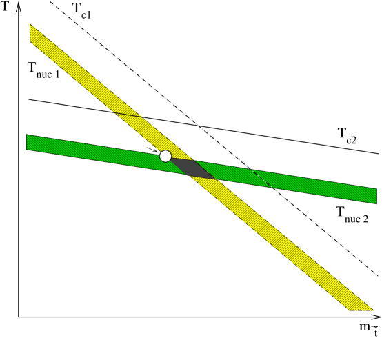
Figure 5: Schematic dependence of critical and bubble nucleation temperatures for the two competing phase transitions (symmetric to CCB and symmetric to electroweak) as a function of squark mass.

The criterion for the symmetric to CCB transition to occur first is that the lower edge of the symmetric to CCB nucleation band be at a higher temperature than the lower edge of the symmetric to EW nucleation temperature band. That is, the symmetric to CCB transition must complete before one electroweak bubble per horizon nucleates out of the symmetric phase. We illustrate this in Figure 5, which shows qualitatively how the two critical temperatures, $T_{ci}$, and the corresponding bubble nucleation temperatures, $T_{{\rm nuc}\ i}$, depend on the right top squark mass $m_{\tilde{t}}$. The temperature for the transition to color breaking (1) depends much more strongly on $m_{\tilde{t}}$ than that for the electroweak transition (2). The open circle in the figure marks the region where the symmetric to CCB transition completes just before nucleation of EW bubbles; it is the optimal point. This choice yields the most shallow possible CCB minimum and thus the greatest probability of being able to make the subsequent transition from CCB to EW phases. The position of the circle illustrates how we choose $m_{\tilde{t}}$ once the other parameters of the MSSM have been specified.

What if we pushed $m_{\tilde{t}}$ a little higher? Then the universe would pass through the diamond in Figure 5, where the nucleation temperature bands overlap. In this case several bubbles of EW phase would nucleate per Hubble volume before the CCB transition completed. If the CCB minimum is deeper at the double nucleation temperature, these bubbles would be absorbed by the CCB phase. But if, as may be the case, the electroweak minimum were the deeper one already at this temperature, then these EW bubbles could continue to expand and eat up the CCB phase. In this case we can get the phenomenology of EW bubbles expanding into a CCB phase, without any CCB to EW bubble nucleations ever occurring. However, this only happens for a very narrow range of values for $\mu^{2}_{s}$, and it also depends on the EW minimum being the deeper one, which is not always the case. This scenario is cosmologically viable and would be quite interesting, but it is highly fine tuned. We will not address it further since the question we want to answer is whether we can get into our EW vacuum after an epoch in which all of space is in the CCB phase.

4.3 CCB to EW transition

Next, let us establish the criterion for judging whether bubble nucleations are efficient enough to get us out of the CCB phase. A rough, conservative requirement is that the nucleation barrier has to be low enough to allow one critical bubble of EW phase per horizon volume per Hubble time, $E/T\simeq 4\ln(T/H)$. As long as the universe is dominated by the energy density of the plasma, $H\sim T^{2}/m_{\rm pl}$. However, at low temperatures the energy density is dominated by the vacuum energy of the CCB phase, which is of order $m_{W}^{4}$. Thus the Hubble constant never gets parametrically smaller than $m_{W}^{2}/m_{\rm pl}$. If we remain in the CCB vacuum when its vacuum energy becomes dominant then the universe begins to inflate. If the nucleation rate continues to be too small at this point, the model is unacceptable for the same reason that old inflation is [16]. Hence a generous criterion is that CCB to EW nucleation never takes place if $E/T$ remains greater than $4\ln(m_{\rm pl}/m_{W})+4\ln 10\simeq 170$, where the extra term $4\ln 10$ is a cushion to insure that our conclusions will be robust.

It is easy to see that nucleation from the CCB to the EW phase can never occur immediately after the CCB phase transition. We already arranged for the symmetric to EW transition to be slower than the symmetric to CCB transition; the CCB to EW transition will be even slower for two reasons:

1. The separation in field space between EW and CCB minima is larger than that between symmetric and EW minima;

2. the CCB minimum is necessarily deeper than the symmetric one at $T_{\rm nuc1}$, so the potential difference between the CCB and EW minima is smaller than between symmetric and EW.

Both of these factors make the CCB $\to$ EW transition slower than the symmetric $\to$ EW one. Therefore if the temperature $T_{\rm nuc3}$ exists, where the CCB phase nucleates copious bubbles of EW phase, it must be considerably below $T_{\rm nuc1}$. The CCB and EW minima become ever deeper and the squark and Higgs condensate values become larger as $T$ falls, so the separation of the minima becomes larger. This is why the high $T$ expansion is not necessarily reliable at $T_{\rm nuc3}$, whereas perturbation theory is more reliable than at the previous phase transition.

We can summarize our procedure as follows. The vacuum theory retains one free parameter we have not yet fixed, $\tilde{A}$ the mixing parameter. We examine values from zero mixing up to the largest $\tilde{A}$ that is compatible with the experimental lower limit on the stop mass. At each value we find the $m_{Q}$ which gives $m_{H}({\rm physical})=95$ GeV and the smallest $\mu^{2}_{s}$ for which the CCB transition happens before the EW one. Then we compute the tunneling action from the CCB to the EW minimum for a range of temperatures between $T_{\rm nuc1}$ and 5 GeV, as well as the vacuum ($T=0$) tunneling action. The bubble action is determined using a new and very efficient algorithm presented in Appendix A. We confirm that tunneling is always inefficient at $T_{\rm nuc1}$; its rate usually peaks at some intermediate temperature, roughly $(2/3)T_{\rm nuc1}$. We also confirm that vacuum tunneling is always extremely inefficient, so much so that typically the thermal tunneling treatment gives the larger (hence correct) value for the rate down to temperatures as low as 3 GeV.

5 Results and Conclusions

In this section we present our results for the energy $E$ of the bubble solutions which interpolate between the CCB and EW vacua, and show that $E/T$ is always larger than the value needed for the phase transition to complete. We will then discuss what kind of new physics might be able to change this conclusion, and the constraints on the MSSM which our analysis implies.

5.1 Results

Using the one loop effective potential with a renormalization point $\overline{\mu}=150{\rm\ GeV}$ intermediate between the top and right stop masses, and at zero squark mixing $\tilde{A}=0$, we find that the minimum value of $E/T$ over temperatures is $1340$, giving a tunneling rate per unit volume of order $T^{4}\exp(-1340)$, which is drastically smaller than the required value of $T^{4}\exp(-170)$. The physical stop mass in this zero-mixing case is $126{\rm\ GeV}$, which is lower than might be expected because of the large downward radiative corrections to $\lambda_{y}$.

         

Figure 6: $E$ in units of $100{\rm\ GeV}$ (solid line) and $E/T$ (dotted line) as a function of temperature, for the critical bubble mediating the CCB to EW phase transition. The left-hand figure is for the case of no mixing and the right-hand figure is maximal mixing, so the right stop mass is $90{\rm\ GeV}$. The vertical bar is $T_{\rm nuc1}$.

Mixing between the left and right stops helps but only weakly; mixing maximally so that the stop mass saturates its experimental bound reduces $E/T$ to $990$, which is still far too large to allow the phase transition to complete. The dependence of the tunneling energy on temperature is shown for each of these cases in Figure 6. The energy of the critical bubble is large at high temperatures and falls monotonically as the temperature is reduced. Likewise the tunneling action is large immediately after the symmetric to CCB transition; in fact, at zero mixing, there is a range of temperatures immediately below $T_{\rm nuc1}$ for which tunneling to the EW minimum is kinematically forbidden. We illustrate the potential as a function of Higgs and squark fields, both at $T_{\rm nuc1}$ and the temperature where $E/T$ is minimized, in Figures 7 and 8.

         

Figure 7: The potential one loop potential, with squark mixing, at $T_{\rm nuc1}$ (left) and at $T$ which minimizes $E/T$ (right). Although the CCB minimum near vacuum becomes quite shallow, it is still not shallow enough to allow efficient nucleation. Note scales; the vertical scales are in units of $(100{\rm\ GeV})^{4}$.

         

Figure 8: This figure is the same as Figure 7 except that there is maximal allowed mixing and two loop effects are included in the effective potential. The CCB transition is stronger, so the CCB minimum is deeper and harder to get out of.

To verify the arguments of section 2.2, we have also checked that our choice of particle masses is optimal. In particular, if the Higgsino or gluino are allowed to be lighter it makes the transition much harder, and if the gluino is heavier the minimum $E/T$ also rises quickly because of the large correction to $\lambda_{s}$. This behavior is shown in Figure 9. Making the Higgsino heavier has a less dramatic effect, but it is also unfavorable to tunneling. To see whether the assumptions about the other particle masses are important, we have pushed the superheavy squark mass scale all the way to $10^{10}{\rm\ GeV}$, and the left stop mass as high as $20{\rm\ TeV}$, obtaining a minimum value of $E/T=1010$ in the zero-mixing limit. This demonstrates that the choice of masses for the very heavy scale particles have no qualitative effect on our conclusions.

Figure 9: Minimum value of the bubble action, $E/T$, as a function of the gluino mass, using the one loop potential and at zero mixing.

We have also checked the robustness of our results with respect to changing the renormalization point. The primary effect of varying $\overline{\mu}$ is to change the thermal contributions to the effective potential, as we have discussed. Setting $\overline{\mu}=90{\rm\ GeV}$ raises the minimum $E/T$ without mixing to 1490; choosing $\overline{\mu}=500{\rm\ GeV}$ lowers $E/T$ to 970 at zero mixing, or 840 at maximal mixing. All of these values are still far from that needed for bubble nucleation. Varying the renormalization point roughly accounts for the uncertainty in $c_{s}$ and $c_{h}$ from two loop effects. The results from the recent paper by Losada [18] show that the best value for the renormalization point is a few times $T$, which is within the range we check here; however we were not able to use the explicit expressions from that paper because it makes different assumptions about what degrees of freedom are heavy. It also uses the high temperature approximation, which as we have stressed is not entirely reliable in the present context.

Another important check is to see how two loop thermal effects change our answers. It has already been observed in previous work that they strengthen the phase transition from the symmetric to the CCB phase [10]. This makes getting out of the CCB phase much harder, both because it increases the required value of $\mu^{2}_{s}$, and because it makes the CCB minimum deep already at a higher temperature. As a result, we find that without mixing, the minimum value of $E/T$ increases to $3000$. Even adding “by hand” a $20\%$ downward contribution to $c_{s}$, the action remains too high, with a minimum $E/T$ of 1220. In fact, getting the minimum $E/T$ down to 170 requires a “by hand” reduction to $c_{s}$ of $45\%$, which two loop effects beyond our leading log treatment cannot possibly provide.

Also, mixing no longer helps when the two loop effects are included. This is because mixing weakens the electroweak transition substantially, since the strength of the latter is set mostly by the coupling of the Higgs to the stop, $\lambda_{y}$; but mixing has little effect on the CCB transition, since its strength comes mainly from gluonic diagrams and not from diagrams involving $\lambda_{y}$. The two loop effects enhance the CCB transition, and if it is very strong and the EW transition is weak, it is more difficult to get out of the CCB minimum. We illustrate this in Figure 8, which is the same as Figure 7 except that it is for maximal mixing and including the two loop effects.

We might also ask, how essential are the experimental bounds on the Higgs and stop masses to our result? The bound on the Higgs mass turns out to be inessential; allowing $m_{h}$ to go down to $65{\rm\ GeV}$ still gives a minimum $E/T=660$, using the one loop potential with mixing, the most favorable combination. However, the bound on the stop mass is essential. If the mixing is large enough, and hence $\lambda_{y}$ small enough, then the second inequality in Eq. (7) will be violated, and the CCB “minimum” will actually be a saddle. However, at high temperatures there may still be a CCB minimum. In this case the universe can go into the CCB minimum safely, because at some temperature the CCB minimum becomes spinodally unstable, and nucleation of EW bubbles is guaranteed to be efficient just above the spinodal temperature. The required value for the stop mass is about $60{\rm\ GeV}$ using the one loop potential and about $50{\rm\ GeV}$ using the two loop potential.

The fact that color breaking is ruled out allows us to exclude some parameter values in the MSSM, namely those for which the color breaking nucleation temperature $T_{\rm nuc1}$ is greater than that of the electroweak transition, $T_{\rm nuc2}$. This condition involves many unknown quantities, such as $\tan\beta$, the Higgs boson mass $m_{h}$, the left stop mass $m_{Q}$, and the stop mixing parameter $\tilde{A}$. We have illustrated the constraint by fixing $\tan\beta=3.2$, while varying $\tilde{A}/m_{Q}$ and $m_{Q}$ in such a way as to keep $m_{h}$ fixed at 95 GeV, and fixing $\tan\beta=7.5$ and keeping $m_{h}=105$ GeV. The excluded region is a stop mass less than some value which depends on $\tilde{A}/m_{Q}$, shown in Figure 10. These are relevant variables because for any value of $m_{\tilde{t}}$, one can always avoid the color breaking transition by making the bare stop mass parameter less negative (i.e., letting $\mu_{s}^{2}$ be smaller), while increasing $\tilde{A}/m_{Q}$. Decreasing $\mu_{s}^{2}$ increases $m_{\tilde{t}}$ while increasing $\tilde{A}/m_{Q}$ does the opposite, so one can keep $m_{\tilde{t}}$ fixed by adjusting the two. To get $m_{h}$ large enough, both $\tilde{A}$ and $m_{Q}$ take values in the TeV. We find that the limiting curves are quite insensitive to the gluino mass.

Figure 10: Our upper limit on the physical stop mass as a function of $(\tilde{A}/m_{Q})^{2}$, for two values of the light Higgs boson mass, using the one-loop effective potential. The region $m_{\tilde{t}}<85$ GeV is separately excluded by accelerator search limits.

5.2 Is there a way out?

The most efficient way of evading our negative result is to find some new physics that decreases the thermal contributions to the right-handed stop Debye mass. Although no such effects are present within the MSSM, one can imagine loopholes in extended models, such as those without $R$-parity. Here we give just one example.

In the absence of $R$-parity, the superpotential includes the baryon number violating terms

$$y^{\prime}_{ijk}\epsilon^{abc}U^{a}_{i}\;D^{b}_{j}\;D^{c}_{k}\,,$$ (42)

involving the right-handed up ($U$) and down ($D$) squark fields of generation $i,j,k$ and color $a,b,c$, with $y^{\prime}_{ijk}$ antisymmetric under $j\leftrightarrow k$. It is possible for $y^{\prime}_{332}$ to be large, if other $R$-parity violating couplings are sufficiently small, without violating any experimental constraints. Associated with the above coupling, one anticipates soft SUSY-breaking terms in the potential of the form

$$y^{\prime}_{332}\;A^{\prime}\;\tilde{t}_{R}^{3}\;(\tilde{b}^{1}_{R}\;\tilde{s}^{2}_{R}-\tilde{b}^{2}_{R}\;\tilde{s}^{1}_{R})\,.$$ (43)

When the stop condenses, $\tilde{t}_{R}^{3}=s$, it induces mixing between the bottom and strange squarks, giving a mass matrix of the form

$$\left(\begin{array}[]{cc}m^{2}_{\tilde{s}}&\pm y^{\prime}A^{\prime}s\\ \pm y^{\prime}A^{\prime}s&m^{2}_{\tilde{b}}\end{array}\right)\,.$$ (44)

Let us consider the situation where there is a hierarchy between the strange and bottom squark diagonal masses, $m^{2}_{\tilde{b}}\gg m^{2}_{\tilde{s}}$. The lighter squark gets a negative correction to its mass eigenvalue from the mixing,

$$m^{2}_{\tilde{s}}\to m^{2}_{\tilde{s}}-{(y^{\prime}A^{\prime}s)^{2}\over m^{2}_{\tilde{b}}}$$ (45)

which makes a negative contribution to the stop thermal mass ($c_{s}T^{2}$) from the one-loop finite temperature potential,

$$\delta c_{s}=-{(y^{\prime}A^{\prime})^{2}\over 6\;m^{2}_{\tilde{b}}}\;.$$ (46)

Although the heavier squark would make an equal and opposite Contribution, it is suppressed if $m_{\tilde{b}}\gg T$. The shift $\delta c_{s}$ could conceivably be large enough to reduce $c_{s}$ by the 45% needed in order to make the CCB to electroweak transition occur.

Another way of thinking of this is that the trilinear term has induced a negative quartic coupling between the strange and stop squarks, analogous to the negative contribution $\tilde{A}$ made to $\lambda_{y}$. A negative coupling between scalars leads to negative thermal masses, which is the physics of thermal symmetry non-restoration. However, for this to work it is essential that there are very large $R$ parity violating effects involving rather light squarks. It is also a little dangerous to induce such a negative effective quartic coupling; it means that there is a very deep extra minimum of the potential in which the right stop, right scalar strange quark, and right scalar bottom quark carry condensates. It is necessary that the universe never nucleates into this minimum, and it may be more problematic to explain the approximate vanishing of the cosmological constant if “our” electroweak minimum is not the global one.

5.3 Conclusions

The phenomenology of electroweak bubbles, in which the Higgs field has a condensate, expanding into a charge and color broken phase where the right stop has a condensate, is potentially rich, and it could be very interesting for baryogenesis. Unfortunately, unless there is new physics beyond the MSSM, this scenario cannot arise by nucleation of EW bubbles out of the CCB phase. We have mentioned $R$-parity violating interactions as one example of such new physics. Another could be the existence of cosmic strings which induce a Higgs field condensate along their cores. Such defects would act like impurities in a solid state system, providing sites for the accelerated nucleation of the electroweak bubbles. The CCB phase can also appear if both phases nucleate out of the symmetric one simultaneously, coexisting for a brief period before the true vacuum state (hopefully electroweak) takes over by squeezing out the CCB bubbles. This latter possibility occurs for such a narrow range of parameter values that we do not consider it to be very compelling.

Thus in the context of the MSSM and barring any additional physics, we conclude that cosmology with a stop squark condensate just before the electroweak phase transition is ruled out. Under these assumptions we can exclude MSSM parameter values, such as those shown in Figure 10, which lead to a CCB phase transition temperature higher than the EW phase transition temperature.

Appendix A Saddle point search algorithms

In this section we will describe two algorithms we use for finding critical bubble actions. One is a general purpose saddle point finding algorithm, mentioned also in the appendix of [19]. The other is special to finding critical bubbles. The second algorithm is highly efficient and to our knowledge it has not appeared previously in the literature.

A.1 General saddlepoint finding algorithm

We want to find a saddle point of a real valued function $H(q_{\alpha})$, where $q_{\alpha}$ are the set of real degrees of freedom (or other continuous variables) on which $H$ depends. In our particular case, the $q_{\alpha}$ are the values of the Higgs and stop fields on a discrete set of points representing radii from $r=0$ out to some $r_{\rm max}$. The Hamiltonian we want to discretize is

$$H=4\pi\int r^{2}dr\left[\frac{1}{2}(\partial_{r}h)^{2}+\frac{1}{2}(\partial_{r}s)^{2}+V(h,s)\right]\,,$$ (47)

where $h$ and $s$ are the Higgs and stop condensates in the real field normalization and $V(s,h)$ is the thermal effective potential. An explicit numerical implementation of $H$ for the present purposes would be to discretize the radius to integer multiples of a discrete spacing $\Delta$ and approximate the energy as

$$\frac{H}{4\pi}=\sum_{i=0}^{i_{\rm max}-1}\frac{i^{2}+i}{2}\Delta\left((h(i+1)-h(i))^{2}+(s(i+1)-s(i))^{2}\right)+\sum_{i=1}^{i_{\rm max}}i^{2}\Delta^{3}V(s,h)\,,$$ (48)

This form for the potential is not essential to the algorithm, though; all we need is for $H$ to depend on a finite number of coordinates and to possess first derivatives which are easy to evaluate numerically.

If we were looking for a minimum of $H$, we could do so by using the “gradient descent” algorithm; pick a starting guess $q_{\alpha}(0)$ for the fields, evaluate the set of derivatives

$$G_{\alpha}(0)\equiv c_{\alpha}\left.\frac{\partial H}{\partial q_{\alpha}}\right|_{q=q(0)}\,,$$ (49)

which comprise the gradient of $H$, and update the fields using

$$q_{\alpha}(1)=q_{\alpha}(0)-\Delta_{\tau}c_{\alpha}G_{\alpha}\,.$$ (50)

Here $\Delta_{\tau}$ is the quenching step length and must be chosen small enough to make the algorithm stable, and the coefficients $c_{\alpha}$ represent a choice of the metric on the space ${q_{\alpha}}$, which should be such that the limiting $\Delta_{\tau}$ to give stability is approximately the same for excitations involving any $q_{\alpha}$; typically $c_{\alpha}\sim\partial^{2}H/\partial q_{\alpha}^{2}$. Then we define $q_{\alpha}(n)$ to be the $n$th iterate of the procedure. This algorithm converges to a minimum.

The usual approach in the literature to find a saddle point is to derive from $H$ equations of motion $E_{\alpha}=\partial H/\partial q_{\alpha}$, and then to define $H^{\prime}=\sum_{\alpha}d_{\alpha}E_{\alpha}^{2}$, with $d_{\alpha}$ some positive coefficients. A saddle point of $H$ is a minimum of $H^{\prime}$, and one can use gradient descent or any other minimum seeking algorithm. However this approach can be inefficient if the saddle point has a very small unstable frequency, and it is also quite cumbersome because $H^{\prime}$ is more complicated than $H$; for instance, if $H$ contains terms with two derivatives, $H^{\prime}$ has terms with four.

We have therefore devised instead an algorithm which deals directly with $H$, and converges rapidly to the desired saddle point. A single iteration of the procedure requires doing the following:

1. Perform $N$ steps of the gradient descent algorithm, with step size $\Delta_{\tau}$.

2. Perform one step of gradient descent with step size $-N\Delta_{\tau}$. Because of the sign, this is actually a “gradient ascent” step, rather than descent.

3. By examining $G_{\alpha}$ before and after, optimize the value of N.

On a “straight slope,” this algorithm does nothing, because the gradient ascent step undoes the gradient descent steps. However, when the second derivatives of $H$ do not vanish, $N$ forward steps are not equivalent to one backward step of $N$ times the length. This is because each forward step starts where the last one stopped. On a concave surface, gradient descent moves towards a stationary point. As the slope becomes smaller, the size of the gradient descent steps becomes smaller. The backward step is then $N$ times as long as the smallest step, and the final configuration is closer to the bottom than the starting one. We illustrate this in Figure 11. On the other hand, on a convex surface, gradient descent moves away from the stationary point, and each step is larger than the previous one. The backward step is $N$ times as large as the largest forward step, and overshoots the starting point. Unless $N$ is too large and it overshoots too much, the algorithm again lands closer to the stationary point. It is to avoid the problem of overshooting in the case where $N\Delta_{\tau}$ is too large that the third step, optimizing $N$, is necessary.

Figure 11: Cartoon showing how the saddle seeking algorithm works. When an extremum is a minimum, gradient descent steps go towards it, and the backwards step is smaller than the series of forward steps. When it is a maximum, the gradient descent moves away, but the backwards step is larger and overshoots, landing closer to the extremum.

Since $H$ is defined in a high dimensional space it is not true that one or the other of the two circumstances mentioned above pertain. Close to an extremum, though, $H$ is approximately a quadratic form in the $q_{\alpha}$, $H\sim H_{\alpha\beta}\delta q_{\alpha}\delta q_{\beta}/2$, and the above arguments apply separately for each eigenvector of $H_{\alpha\beta}$. More generally, unless $N\Delta_{\tau}$ is very large, the algorithm will always go uphill along directions with negative curvature and downhill along directions with positive curvature, which will lead it towards a region with smaller gradients, and hence towards some extremum.

Now we will describe the procedure for optimizing $N$. First, one notices that if the departure from the saddle point is predominantly in convex (stable) directions then we get closer to the minimum fastest simply by using gradient descent without backward steps. It is also easy to tell if this is the case; when it is, $\sum_{\alpha}G_{\alpha}G_{\alpha}$ diminishes with each forward step. For this reason, and because the unstable frequency of a critical bubble is typically lower than any of the stable frequencies, we will concentrate on the case where almost all that is left is departure from the saddle in the unstable direction. One iteration of the algorithm multiplies the departure from the saddle in the unstable direction by $(1-x)\exp(x)$, where $x=N\Delta_{\tau}\omega_{-}^{2}$ and $\omega_{-}$ is the unstable frequency of the saddle point. The algorithm overshoots if $x>1$ and it is unstable if $x>1.278$. However, we can measure the extent of overshoot or undershoot by comparing the gradient after an iteration of the algorithm, $G_{\alpha}({\rm after})$, with the gradient before, $G_{\alpha}({\rm before})$. Our indicator of whether $N$ is too large is

$$\frac{\sum_{\alpha}G_{\alpha}({\rm after})G_{\alpha}({\rm before})}{\sum_{\alpha}G_{\alpha}({\rm before})^{2}}\,;$$ (51)

if this is positive, we can safely increase $N$, and if it is negative we must reduce $N$. If there are no remaining excitations in stable directions then the value of the indicator will be $(1-x)\exp(x)$, which makes it easy to choose a new value of $N$ which will make $x$ very close to 1. When $x=1$, the algorithm “steps back” just the right distance and lands on the saddle point. It is also possible to determine the unstable frequency from the value of $N\Delta_{\tau}$ which worked optimally.

As with any saddle point finding algorithm it is still necessary to feed in a good starting guess so that the algorithm finds the right extremum of the action. Here we have little new to say. Our approach has been to define a few-parameter Ansatz for a path in field space between the EW and CCB vacua, and to use a shooting algorithm to find the action for each value of the parameters. Then we minimize the action over the parameters in the Ansatz. All that is necessary is that the starting guess not be terribly bad, although in practice the saddle finding algorithm converges faster if the starting guess is better.

A.2 Efficient algorithm just for multi-field critical bubbles

Now we describe a much more efficient algorithm, which is however special to the problem of determining critical bubble configurations and actions in theories with more than one field. The general problem is to find the lowest saddle point of the Hamiltonian

$$H=4\pi\int r^{2}dr\left(\sum_{i}\frac{(\partial_{r}f_{i}(r))^{2}}{2}+V(f_{i}(r))\right)\,,$$ (52)

where $f_{i}$ represent several fields which may all have condensates, and the boundary conditions are that the $f_{i}$ start at $r=0$ near the true minimum and approach their false vacuum values at large $r$. Although we have in mind a numerical implementation involving discretization of $r$, we use the simpler continuum notation.

The problem reduces to the one field case if we consider a restricted set of configurations in which the fields always lie along a one dimensional trajectory through field space. That is, we choose a curve in the space of $\{f_{1},\ldots,f_{n}\}$, parameterized by a path length $l$, $f_{i}=f_{i}(l)$. By path length we mean that $l$ is chosen so that

$$\sum_{i}\left(\frac{df_{i}(l)}{dl}\right)^{2}=1\,.$$ (53)

Then we require that the fields $f_{i}(r)$ can be written as $f_{i}(l(r))$. This is the same as making all of the fields dependent on the value of one field. For this restricted set of configurations, the Hamiltonian is

$$H({\rm restricted})=4\pi\int r^{2}dr\left[\frac{1}{2}\left(\frac{dl}{dr}\right)^{2}+V(f_{i}(l(r)))\right]\,.$$ (54)

The standard shooting algorithm finds the saddle point on this restricted class of configurations, and its action is an upper bound for the true saddlepoint action. The “only” remaining problem is to find the minimum over all choices of paths in field space.

This is where the gradient descent algorithm comes in. If our choice of path is imperfect, the shooting algorithm gives a bubble configuration which is not a true saddle point. So, lifting the requirement that the fields lie on any prescribed path in field space, gradient descent will lead to a lower energy configuration which must, at least initially, be following a “better” path through field space, meaning one which will give a lower saddle point energy. This leads to the following algorithm. First, we choose some “reasonable” path through field space. We evaluate the potential at a series of points along it and define the potential to be the spline interpolation of those points. Then we iterate the following procedure:

1. Find the saddle point solution for the particular path through field space by the standard “shooting” algorithm;

2. Apply a reasonably short amount of gradient descent cooling to the resulting configuration, making no requirements that the fields remain on any trajectory in field space;

3. Use the $f_{i}(r)$ after the gradient descent to define a new choice for a path through field space. In practice we know $f_{i}$ at a discrete set of radii $r$, so we take the path to be the series of straight line segments joining the points $f_{i}(r_{\rm known})$, and the potential to be the spline interpolation of $V(f_{i}(r))$.

We illustrate how the iteration converges to the “right” path through field space in Figure 12, which shows a series of paths in field space from iterations of the above algorithm. In our case there are only two fields, but the algorithm generalizes immediately to many fields.

Figure 12: An example of how the second algorithm converges to the right line through field space. The starting guess for the line through field space is the leftmost one with a sharp angle, and each line in the series represents the result of one more iteration of the algorithm. The algorithm converges quickly to the right line through field space.

Apart from step size errors, the algorithm converges to a saddle point configuration with only one unstable direction. This is because the shooting procedure only allows one unstable mode, associated with variations in dependence of the fields on the radius while staying on the same path, and the gradient descent algorithm does not tolerate any unstable modes for which the fields leave the path. There is no guarantee that we will find the lowest action; if there are several saddlepoint solutions with only one unstable direction, the one we find depends on the basin of attraction in which the starting guess for a path lies. This is a general problem with any saddle point seeking algorithm. However we have not found it to be a problem in practice.

We have compared this algorithm with the one described in the last subsection. They converge to the same solutions and give the same saddle point energy to about $1\%$ accuracy for the step size we use. It is easier to make the general algorithm give higher accuracy; one recomputes the action with half the step size and extrapolates to zero step size assuming $O(\Delta^{2})$ errors. This leaves a very small $O(\Delta^{4})$ error which in practice can be made of order $10^{-4}$ quite easily. We have been less successful bringing the errors of the algorithm presented here below $O(\Delta^{2})$. However, the algorithm efficiency is drastically better, especially when the saddle point action is large; and since we are neglecting corrections (such as vacuum two-loop contributions to $V$, field dependent wave function corrections, and higher derivative corrections) which enter at the $1\%$ level we see little point in pursuing numerical accuracy further.

Appendix B Renormalization Group choice of couplings

Here we discuss the renormalization group analysis, used to determine the scalar couplings at a renormalization point $\overline{\mu}$. To begin with, we need values for the strong and Yukawa couplings. We take the value of the strong coupling in the five quark scheme at the $Z$ pole, $\alpha_{s}(91{\rm\>GeV},\overline{\rm MS})=0.118$, and convert it to $\overline{\rm DR}$ in the six quark plus right squark scheme using the relation [20]

$$g_{s}^{2}(M_{Z},\overline{\rm DR},6{\rm\;quark+right\;squark}) = \frac{\alpha_{s}(M_{Z},\overline{\rm MS},5{\rm\;quark})}{1-\Delta\alpha_{s}}\,,$$ (55)

$$\Delta\alpha_{s} = \frac{\alpha_{s}}{2\pi}\left[\frac{1}{2}-\frac{2}{3}\ln\frac{m_{t}}{m_{Z}}-\frac{1}{6}\ln\frac{m_{s}}{m_{Z}}\right]\,,$$ (56)

which coincidentally gives almost the same value. We run this to the top mass using the one loop beta function, to be given shortly. We also determine the Yukawa coupling at $\overline{\mu}=m_{t}$ from the expression [20]

$$\frac{y\sin\beta(\overline{\rm DR},\overline{\mu}=m_{t})}{\sqrt{2}}=\frac{m_{t}}{v}\left(1-\frac{5g_{s}^{2}}{12\pi^{2}}\right)\,.$$ (57)

In $\overline{\rm MS}$ the $5$ would be a $4$. We define $\beta$ so that $\sin\beta$ is the overlap between the light and up-type ($H_{2}$) Higgs eigenstates using the wave functions at the renormalization point set by the heavy Higgs field threshold; below the threshold only the combination $y\sin\beta$, which is the coupling of the light Higgs to the top quark, appears. The exception is the top-stop-Higgsino coupling, which we approximate to be $1/\sin\beta$ times the Higgs-top-top coupling.

We run $g_{s}^{2}$ and $y^{2}$ to the ultraviolet using one loop beta functions, including only strong and Yukawa contributions in the beta functions, and putting each heavy particle into loops after crossing its threshold. At the energy scale of the heaviest particle, we relate $\lambda_{s}$ and $\lambda_{h}$ to the gauge couplings using the SUSY relations, given in the main text in Eq. (11); similarly

$$\lambda_{y}(\overline{\mu}=UV)=y^{2}-\frac{1}{3}g^{\prime 2}$$ (58)

fixes $\lambda_{y}$ above all thresholds. These SUSY relations hold at this UV scale, although if we had used $\overline{\rm MS}$ there would be nonlogarithmic one loop corrections. Then we run all 5 couplings back down to the infrared, switching to the effective theory without a heavy particle when we cross its mass threshold. We allow ourselves the approximation that the Yukawa-like couplings of gluinos and Higgsinos equal the respective strong and Yukawa couplings. Although these relationships are actually broken below heavy particle thresholds we believe that this produces only a small error. We also systematically drop electroweak contributions to the beta functions.

The procedure is possible because the strong and Yukawa beta functions do not depend on the scalar self-couplings; otherwise we would have to seek UV values of $g_{s}^{2}$ and $y^{2}$ which would “hit” the appropriate IR values. The procedure is necessary because our choices for particle masses lead to large logarithms like $\log(m_{Q}/m_{t})\simeq 4$, which makes it important to include, for instance, two-loop $\log^{2}$ contributions. The difference between performing the renormalization group analysis and simply enforcing the SUSY relations between the couplings at our infrared renormalization point is a shift of order $20\%$ in $\lambda_{s}$ and $\lambda_{y}$, and of course a larger shift in $\lambda_{h}$, which has a small SUSY value at low $\tan\beta$ but large radiative corrections from the Yukawa coupling. The residual two loop and electroweak errors left out from our analysis should be of order a few percent.

Now we present the complete expressions for the beta functions. The simplest is the strong beta function,

$$\beta_{g_{s}^{2}} = \frac{g_{s}^{4}}{16\pi^{2}}\left\{-\frac{41}{3}+4\;\theta(\overline{\mu}-m_{\tilde{g}})+\frac{2}{3}\;\theta(\overline{\mu}-m_{Q})+3\;\theta(\overline{\mu}-m_{\rm heavy})\right\}\,.$$ (59)

Here $-41/3$ is the value in the six quark standard model plus right stop, and the $\theta$ functions turn on each particle’s contribution as $\overline{\mu}$ passes its mass threshold; the sum of the terms is $-6$, which is the correct expression in the full SUSY theory.

The expressions for the other couplings are less elegant; for the Yukawa coupling we have

$$\beta_{y^{2}} = \frac{y^{2}}{16\pi^{2}}\Bigg{[}9y^{2}\sin^{2}\beta-16g_{s}^{2}+9y^{2}\cos^{2}\!\beta\,\theta(\overline{\mu}-m_{A^{0}})+$$ (60)

$$+\left(2y^{2}+\frac{8}{3}g_{s}^{2}\right)\theta(\overline{\mu}-m_{Q})+y^{2}\theta(\overline{\mu}-m_{\tilde{h}})+\frac{8}{3}\;g_{s}^{2}\theta(\overline{\mu}-m_{\tilde{g}})\Bigg{]}\,,$$

where the dependence on $m_{A^{0}}$ is because we actually change what we mean when we cross its threshold. Above the $A^{0}$ threshold, the Yukawa coupling is the coupling of the up-type ($H_{2}$) Higgs field to the tops; below, $y^{2}\sin^{2}\beta$ is the coupling of the light Higgs field to the tops. The expression below all mass thresholds agrees with the standard model value and the result above thresholds agrees with the MSSM result.

The expressions for the scalars are even more complicated. For the squark self-coupling, and using SUSY relations for its couplings via D terms to other squarks (which are heavy, so the SUSY relations hold when it matters), we have

$$\beta_{\lambda_{s}} = \frac{1}{16\pi^{2}}\Bigg{[}\frac{13}{6}g_{s}^{4}-16g_{s}^{2}\lambda_{s}+28\lambda_{s}^{2}+2\lambda_{y}^{2}+\frac{3}{2}g_{s}^{4}\theta(\overline{\mu}-m_{\rm heavy})+$$ (61)

$$+\left(\frac{1}{3}g_{s}^{4}-\frac{4}{3}g_{s}^{2}y^{2}+2y^{4}\right)\theta(\overline{\mu}-m_{Q})+\left(\frac{32}{3}g_{s}^{2}\lambda_{s}-\frac{44}{9}g_{s}^{4}\right)\theta(\overline{\mu}-m_{\tilde{g}})$$

$$+(8y^{2}\lambda_{s}-4y^{4})\theta(\overline{\mu}-m_{\tilde{h}})\Bigg{]}\,,$$

where the reader should be cautious because the meaning of $\lambda_{y}$ in this expression changes at $m_{A^{0}}$ and $m_{Q}$; at $m_{A^{0}}$ it goes from being the coupling between the up-type Higgs and stop to that of the light Higgs and stop, and at $m_{Q}$ it is modified by mixing, reducing it by a factor of $1-(\tilde{A}^{2}/m_{Q}^{2})$. As previously noted we assume $m_{A^{0}}=m_{Q}$ for simplicity.

To match $\lambda_{y}$ across the $m_{Q}$ threshold, we require that $m_{A^{0}}=m_{Q}$. There are two threshold effects; first, the coupling of the light Higgs below the threshold is $\sin^{2}\!\beta$ times the coupling of the up type Higgs to the stop, plus $\cos^{2}\!\beta$ times the coupling of the down type Higgs to the stop, which is $g^{\prime 2}/3$. Also, there is the mixing induced by the diagram in Figure 2. The matching condition across the threshold is therefore

$$\lambda_{y}({\rm below})=\lambda_{y}({\rm above})\sin^{2}\!\beta+\frac{g^{\prime 2}}{3}\cos^{2}\!\beta-y^{2}\sin^{2}\!\beta\frac{\tilde{A}^{2}}{m_{Q}^{2}}\,.$$ (62)

The expression for the beta function of $\lambda_{y}$, valid both above and below the $m_{A^{0}}$ threshold, is

$$\beta_{\lambda_{y}} = \frac{1}{16\pi^{2}}\Bigg{[}6\lambda_{y}y^{2}\sin^{2}\!\beta+(4\lambda_{y}+12\lambda_{h}+16\lambda_{s}-8g_{s}^{2})\lambda_{y}+2y^{4}\theta(\overline{\mu}-m_{Q})+$$ (63)

$$\left(6y^{2}\lambda_{y}-\frac{32}{3}g_{s}^{2}-4y^{4}\right)\cos^{2}\!\beta\theta(\overline{\mu}-m_{A^{0}})+(4y^{2}\lambda_{y}-4y^{4}\sin^{2}\!\beta)\theta(\overline{\mu}-m_{\tilde{h}})$$

$$+\left(\frac{16}{3}g_{s}^{2}\lambda_{y}-\frac{32}{3}g_{s}^{2}y^{2}\sin^{2}\!\beta\right)\theta(\overline{\mu}-m_{\tilde{g}})\Bigg{]}\,.$$

Including $\lambda_{h}$ effects in the beta function for $\lambda_{y}$ is slightly inconsistent because $\lambda_{h}$ is largely an electroweak effect and the canceling electroweak effect required by SUSY is missing since we ignore electroweak couplings. However the error this causes is negligible because $3\lambda_{s}\lambda_{h}/(4\pi^{2})$ is numerically very small compared to $\lambda_{y}$.

Lastly there is the beta function for $\lambda_{h}$. It barely runs above $m_{Q}$, so we enforce its SUSY relation there, choosing the value just below to be $(g^{2}+g^{\prime 2})\cos^{2}(2\beta)/8$. Below both $m_{Q}$ and $m_{A^{0}}$ thresholds, we run it using the beta function

$$\beta_{\lambda_{h}}=\frac{1}{16\pi^{2}}\Bigg{[}3\lambda_{y}^{2}-6y^{4}\sin^{4}\beta+12y^{2}\lambda_{h}\sin^{2}\beta\Bigg{]}\,.$$ (64)

The electroweak correction to $\lambda_{h}$ from the very heavy squarks is not entirely negligible, because of the large log and because $\lambda_{h}$ is not very big; it shifts the final value of $\lambda_{h}$ by about $5\%$ of the SUSY value. We have neglected this effect in our work, as part of consistently dropping electroweak radiative corrections, which is reasonable because the Yukawa type corrections to $\lambda_{h}$ are of order 1.

References

- [1] A. Sakharov, JETP Lett. 6, 24 (1967).
- [2] G. t’Hooft, Phys. Rev. Lett. 37,8 (1976).
- [3] V. Kuzmin, V. Rubakov, and M. Shaposhnikov, Phys. Lett. D 30, 36 (1985); P. Arnold and L. McLerran, Phys. Rev. D 36, 581 (1987); J. Ambjørn and A. Krasnitz, Phys. Lett. B 362, 97 (1995); G. D. Moore, C. Hu, and B. Müller, Phys. Rev. D 58, 045001 (1998).
- [4] M. Gavela, P. Hernandez, J. Orloff, and O. Pene, Nucl. Phys. B 430 (1994) 345; M. Gavela, P. Hernandez, J. Orloff, O. Pene, and C. Quimbay, Nucl. Phys. B 430 (1994) 382.
- [5] G. D. Moore, MCGILL-98/7, hep-ph/9805264.
- [6] R. Clare, L3 report to LEPC, http://l3www.cern.ch/conferences/talks98.html
- [7] K. Kajantie, M. Laine, K. Rummukainen, and M. Shaposhnikov, Phys. Rev. Lett. 77, 2887 (1996); M. Gürtler, E. Ilgenfritz, and A. Schiller, Phys. Rev. D 56, 3888 (1997); K. Rummukainen, M. Tsypin, K. Kajantie, M. Laine, and M. Shaposhnikov, Nucl. Phys. B532, 283 (1998); F. Csikor, Z. Fodor, and J. Heitger, Phys. Rev. Lett. 82, 21 (1999);
- [8] J. R. Espinosa, Nucl.Phys. B 475 273, (1996); B. de Carlos and J. R. Espinosa, Nucl. Phys. B 503, 24 (1997); M. Carena, M. Quirós, and C.E.M. Wagner, Nucl. Phys. B 524, 3 (1998); D. Bödeker, P. John, M. Laine and M.G. Schmidt, Nucl. Phys. B497, 387 (1997); J. Cline and G. D. Moore, Phys. Rev. Lett. 81, 3315-3318 (1998), hep-ph/9806354; M. Losada, hep-ph/9806519; M. Laine and K. Rummukainen, hep-lat/9804019; Phys. Rev. Lett. 80, 5259 (1998).
- [9] A. Kusenko, P. Langacker and G. Segre, Phys. Rev. D54, 5824 (1996).
- [10] D. Bödeker, P. John, M. Laine and M.G. Schmidt, Nucl. Phys. B497, 387 (1997).
- [11] M. Carena, M. Quirós, and C.E.M. Wagner, Nucl. Phys. B 524, 3 (1998).
- [12] I. Affleck, Phys. Rev. Lett. 46, 388 (1981).
- [13] S. Coleman, Phys. Rev. D 15, 2929 (1977); C. Callan and S. Coleman, Phys. Rev. D 16, 1762 (1977).
- [14] J. Cline and P.-A. Lemieux, Phys. Rev. D55, 3873 (1997).
- [15] D. Comelli and J. Espinosa, Phys. Rev. D 55, 6253 (1997).
- [16] A. Guth and E. Weinberg, Nucl. Phys. B 212, 321 (1983).
- [17] J. Baacke, Phys. Rev. D 52, 6760 (1995).
- [18] M. Losada, Nucl. Phys. B 537, 3 (1999), hep-ph/9806519.
- [19] J. Cline, J. Espinosa, G. D. Moore, and A. Riotto, CERN-TH-98-306, hep-ph/9810261.
- [20] D. Pierce, J. Bagger, K. Matchev, and R. Zhang, Nucl. Phys. B 491, 3 (1997).