The $B\rightarrow X_{d}\,\ell^{+}\ell^{-}$ decay in general two Higgs doublet model

The branching ratio, forward–backward asymmetry and CP violating asymmetry for $B\rightarrow X_{d}\,\ell^{+}\ell^{-}$ decay, in framework of the general two Higgs doublet model, with extra phase angle in the charged–Higgs–fermion coupling, are calculated. It is shown that studying the CP violating asymmetry is an efficient tool for establishing new physics.

1 Introduction

Rare $B$ meson decays, induced by the flavor–changing neutral current (FCNC) $b\rightarrow s\,(d)$ transitions is one of the most promising research area in particle physics. Theoretical interest to the rare $B$ decays lies in their role as a potential precision testing ground for the Standard Model (SM) at loop level. Experimentally, these decays will provide a more precise determination of the elements of the Cabibbo–Kobayashi–Maskawa matrix (CKM), such as $V_{tq},~{}(q=d,~{}s,~{}b)$ and $V_{ub}$ and $CP$ violation.

The impressive experimental search for the study of the $B$ meson decay will be carried out in future, when new experimental facilities, especially the $B$–factories at Belle [1] and BaBar [2], are upgraded, and after which the large number $(10^{8}$–$10^{12})$ of B hadrons that is expected to be produced in these factories, will allow measuring the FCNC decays of B mesons.

In the first hand, the most reliable quantitative test of FCNC in $B$ meson decays is expected to be measured in the $B\rightarrow X_{s(d)}\ell^{+}\ell^{-}$ decay. The matrix elements of the $b\rightarrow s\ell^{+}\ell^{-}$ transition contains terms describing the virtual effects by $t\bar{t}$, $c\bar{c}$ and $u\bar{u}$ loops which are proportional to combination of the CKM elements $V_{tb}V_{ts}^{\ast}$, $V_{cb}V_{cs}^{\ast}$ and $V_{ub}V_{us}^{\ast}$ respectively. Using the unitarity condition of the CKM matrix and neglecting $V_{ub}V_{us}^{\ast}$ in comparison to $V_{tb}V_{ts}^{\ast}$ and $V_{cb}V_{cs}^{\ast}$, it is obvious that the matrix element for the $b\rightarrow s\ell^{+}\ell^{-}$ decay involves only one independent CKM matrix factor, $V_{tb}V_{ts}^{\ast}$, so that CP–violation in this channel is strongly suppressed in the SM.

The situation is totally different for the $b\rightarrow d\ell^{+}\ell^{-}$ decay, since all three CKM factors are of the same order in SM, and therefore can induce considerable CP violation in the decay rate difference of the $b\rightarrow d\ell^{+}\ell^{-}$ and $\bar{b}\rightarrow\bar{d}\ell^{+}\ell^{-}$ processes (for the current status of $B\rightarrow X_{s(d)}\ell^{+}\ell^{-}$ decay in SM, see [3] and the references therein). So, the $b\rightarrow d\ell^{+}\ell^{-}$ is a promising decay for establishing CP violation in B mesons.

The rare B meson decays are also very sensitive to the ’new physics’ beyond SM, such as the two Higgs doublet model (2HDM), minimal supersymmetric extension of the SM (MSSM) [4], etc.

One of the most popular extension of the SM is the 2HDM [5], which contains two complex Higgs doublets rather than one, as is the case in the SM. In the 2HDM, the FCNC that appear at the tree level, are avoided by imposing an ad hoc discrete symmetry [6]. One possible way to avoid these unwanted FCNC at tree level, is to couple all fermions to only one of the two Higgs doublets (Model I). The other possibility is the coupling of the up and down quarks to the first and second doublets, respectively (Model II).

Models I and II have been extensively investigated theoretically and tested experimentally (see [5] and references therein). The 2HDM without the ad hoc discrete symmetry was analyzed in [7]–[9]. It is clear that the tree level FCNC appears in this model, however their couplings involving first and second generations must be strongly suppressed. This conclusion is the result of the analysis of low energy experiments. Therefore, Model III should be parametrized in a way that suppresses the tree level FCNC couplings of the first generation, while the tree level FCNC couplings involving the third generation can be made non–zero as long as they do not violate the existing experimental data, i.e., $B$–$\bar{B}^{0}$ mixing.

In this work, following [7], we assume that all tree level FCNC couplings are negligible. However, even under this assumption, the couplings of fermions with Higgs bosons may have a complex phase $e^{i\theta}$ (see [7] and [10]). The constraints on the phase angle $\theta$ in the product $\lambda_{tt}\lambda_{bb}$ (see below) of Higgs–fermion couplings imposed by the neutron electric dipole moment, $B$–$\bar{B}^{0}$ mixing, $\rho_{0}$ parameter and $b\rightarrow s\gamma$ decay are discussed in [7].

The aim of the present work is the quantitative investigation of the CP violation in the inclusive $B\rightarrow X_{d}\,\ell^{+}\ell^{-}$ decay in context of the general 2HDM, in which a new phase parameter is present (see below). In other words, this model contains a new source of CP violation whose interference with the SM phase can induce considerable difference in the CP violation predicted by the SM. To find an answer to the question of, ”to what extend the new physics effects the results of the SM”, is the main goal of the present work.

The paper is organized as follows. In Sect. 2, we present the necessary theoretical background for the general 2HDM and calculate the branching ratio, CP violation and forward–backward asymmetry in the $b\rightarrow d\ell^{+}\ell^{-}$ decay. Finally, Sect. 3 is devoted to the numerical analysis and concluding remarks.

2 The formalism

Before presenting the necessary theoretical expressions for studying $b\rightarrow d\ell^{+}\ell^{-}$ decay, let us briefly remind the main essential points of the Model III. In this model, without loss of generality, we can choose a basis such that the first Higgs doublet creates all fermion and gauge boson masses, whose vacuum expectation values are

$$\left<H_{1}\right>=\left(\begin{array}[]{c}0\\ \\ \displaystyle{\frac{v}{\sqrt{2}}}\end{array}\right)~{}~{},~{}~{}~{}~{}~{}\left<H_{2}\right>=0~{}.$$ (4)

In this basis the first doublet $H_{1}$ is the same as in the SM, and all new Higgs bosons result from the second doublet $H_{2}$, which can be written as

$$H_{1}=\frac{1}{\sqrt{2}}\left(\begin{array}[]{c}\sqrt{2}\,G^{+}\\ \\ v+\chi_{1}^{0}+iG^{0}\end{array}\right)~{}~{},~{}~{}~{}~{}~{}H_{2}=\frac{1}{\sqrt{2}}\left(\begin{array}[]{c}\sqrt{2}\,H^{+}\\ \\ \chi_{2}^{0}+iA^{0}\end{array}\right)~{},$$ (11)

where $G^{+}$ and $G^{0}$ are the Goldstone bosons. The neutral $\chi_{1}^{0}$ and $\chi_{2}^{0}$ are not the physical basis, but their linear combination gives the physical neutral $H^{0}$ and $h^{0}$ Higgs bosons:

$$\chi_{1}^{0}=H^{0}\cos\alpha-h^{0}\sin\alpha~{},$$

$$\chi_{2}^{0}=H^{0}\sin\alpha+h^{0}\cos\alpha~{}.$$

The general Yukawa Lagrangian can be written as

$${\cal L}_{Y}=\eta_{ij}^{U}\bar{Q}_{iL}\widetilde{H}_{1}U_{jR}+\eta_{ij}^{\cal D}\bar{Q}_{iL}H_{1}{\cal D}_{jR}+\xi_{ij}^{U}\bar{Q}_{iL}\widetilde{H}_{2}U_{jR}+\xi_{ij}^{\cal D}\bar{Q}_{iL}H_{2}{\cal D}_{jR}+h.c.~{},$$ (12)

where $i$, $j$ are the generation indices, $\widetilde{H}_{1,2}=i\sigma_{2}H_{1,2}$, $\eta_{ij}^{U,{\cal D}}$ and $\xi_{ij}^{\cal U,D}$, in general, are the non–diagonal coupling matrices, $Q_{iL}$ is the left–handed fermion doublet, $U_{R}$ and $D_{R}$ are the right–handed singlets. In Eq. (1) all states are weak states, that can be transformed to the mass eigenstates by rotation. After this rotation is performed, the Yukawa Lagrangian takes the following form (only the part of the Yukawa Lagrangian that is relevant to our analysis)

$${\cal L}_{Y}=-H^{+}\bar{U}\left[V_{CKM}\hat{\xi}^{\cal D}R-\hat{\xi}^{U^{+}}V_{CKM}L\right]{\cal D}~{}.$$ (13)

The FCNC couplings are contained in the matrices $\hat{\xi}^{U^{+},{\cal D}}$. In the present analysis, we will use a simple ansatz for $\hat{\xi}^{U^{+},{\cal D}}$ [8],

$$\hat{\xi}^{U,{\cal D}}=\lambda_{ij}\frac{g\sqrt{m_{i}m_{j}}}{\sqrt{2}m_{W}}~{},$$ (14)

This ansatz guarantees that FCNC for the first generations are strongly suppressed since it is proportional to the small quark mass. It follows from Eq. (3) that, we can safely neglect the neutral Higgs boson exchange diagrams, and only charged Higgs boson gives new contribution to the $b\rightarrow d\ell^{+}\ell^{-}$ decay. Note that $\lambda_{ij}$ are complex parameters of order ${\cal O}(1)$ (see [7]), i.e., $\lambda_{ij}=\left|\lambda_{ij}\right|e^{i\theta}$. Being complex, $\lambda_{ij}$ allow the charged Higgs boson to interfere destructively or constructively to the SM results. In other words, branching ratio, as well as CP asymmetry, can get increased or decreased for the $b\rightarrow d\ell^{+}\ell^{-}$ decay in Model III. For simplicity we choose $\hat{\xi}^{U,{\cal D}}$ to be diagonal to suppress all tree level FCNC couplings, and as a result $\lambda_{ij}$ are also diagonal but remain complex. Note that the results for Model I and Model II can be obtained from Model III by the following substitutions:

$$\lambda_{tt}=\cot\beta~{}~{}~{}~{}~{}~{}~{}\lambda_{bb}=-\,\cot\beta~{}~{}\mbox{\rm for Model I}~{},$$

$$\lambda_{tt}=\cot\beta~{}~{}~{}~{}~{}~{}~{}\lambda_{bb}=+\,\tan\beta~{}~{}\mbox{\rm for Model II}~{}.$$ (15)

After these preliminary remarks, let us return our attention to the $b\rightarrow d\ell^{+}\ell^{-}$ decay. The powerful framework into which the perturbative QCD corrections to the physical decay amplitude incorporated in a systematic way, is the effective Hamiltonian method. In this approach, the heavy degrees of freedom in the present case, i.e., $t$ quark, $W^{\pm},~{}H^{\pm},~{}h^{0},~{}H^{0}$ are all integrated out. The procedure is to match the full theory with the effective theory at high scale $\mu=m_{W}$, and then calculate the Wilson coefficients at lower $\mu\sim{\cal O}(m_{b})$ using the renormalization group equations. In our calculations we choose the higher scale as $\mu=m_{W}$, since In the version of the 2HDM we consider in this work, the charged Higgs boson the charged Higgs boson is heavy enough ($m_{H^{\pm}}\geq 210~{}GeV$ see [11]) to neglect the evolution from $m_{H^{\pm}}$ to $m_{W}$. In the version of the 2HDM we consider in this work, the charged Higgs boson exchange diagrams do not produce new operators and the operator set is the same as the one used for the $b\rightarrow d\ell^{+}\ell^{-}$ decay in the SM, but the values of the Wilson coefficients are changed at $m_{W}$ scale. The effective Hamiltonian for the $b\rightarrow d\ell^{+}\ell^{-}$ decay is The effective Hamiltonian for the $b\rightarrow d\ell^{+}\ell^{-}$ decay is [12, 13]

$${\cal H}=-4\frac{G_{F}}{2\sqrt{2}}V_{tb}V^{*}_{td}\left\{\sum_{i=0}^{10}C_{i}(\mu)O_{i}(\mu)+\lambda_{u}\sum_{i=1}^{2}C_{i}(\mu)\left[O_{i}(\mu)-O_{i}^{u}(\mu)\right]\right\}~{},$$

where

$$\lambda_{u}=\displaystyle{\frac{V_{ub}V^{*}_{ud}}{V_{tb}V^{*}_{td}}}~{},$$

and $C_{i}$ are the Wilson coefficients. The explicit form of all operators $O_{i}$ can be found in [12, 13]. Using the effective Hamiltonian, the matrix element of the $b\rightarrow d\ell^{+}\ell^{-}$ decay takes the following form:

$${\cal M} = \frac{G_{F}\alpha}{2\sqrt{2}\pi}V_{td}V^{*}_{tb}\Bigg{\{}C_{9}^{eff}\bar{d}\gamma_{\mu}(1-\gamma_{5})b\,\bar{\ell}\gamma^{\mu}\ell+C_{10}\bar{d}\gamma_{\mu}(1-\gamma_{5})b\,\bar{\ell}\gamma^{\mu}\gamma_{5}\ell$$ (16)

$$- 2C_{7}^{eff}\frac{m_{b}}{p^{2}}\bar{d}i\sigma_{\mu\nu}p^{\nu}(1+\gamma_{5})b\,\bar{\ell}\gamma^{\mu}\ell\Bigg{\}}~{},$$

where $q^{2}=(p_{1}+p_{2})^{2}$ is the invariant dilepton mass squared, $p_{1}$ and $p_{2}$ are the four–momentum of leptons. In Eq. (5) all Wilson coefficients are evaluated at the $\mu=m_{b}$ scale. As has already been noted earlier, in the model under consideration the charged Higgs boson contributions to leading order at $\mu=m_{W}$ scale modify only values of the Wilson coefficients, i.e.,

$$C_{7}^{2HDM}(m_{W}) = C_{7}^{SM}(m_{W})+C_{7}^{H^{\pm}}(m_{W})$$

$$C_{9}^{2HDM}(m_{W}) = C_{9}^{SM}(m_{W})+C_{9}^{H^{\pm}}(m_{W})$$

$$C_{10}^{2HDM}(m_{W}) = C_{10}^{SM}(m_{W})+C_{10}^{H^{\pm}}(m_{W})~{}.$$

The coefficients $C_{i}^{2HDM}(m_{W})$ to the leading order are given by

$$C_{7}^{2HDM}(m_{W}) = x\,\frac{(7-5x-8x^{2})}{24(x-1)^{3}}+\frac{x^{2}(3x-2)}{4(x-1)^{4}}\,\ln x$$ (17)

$$+ \left|\lambda_{tt}\right|^{2}\Bigg{(}\frac{y(7-5y-8y^{2})}{72(y-1)^{3}}+\frac{y^{2}(3y-2)}{12(y-1)^{4}}\,\ln y\Bigg{)}$$

$$+ \lambda_{tt}\lambda_{bb}\Bigg{(}\frac{y(3-5y)}{12(y-1)^{2}}+\frac{y(3y-2)}{6(y-1)^{3}}\,\ln y\Bigg{)}~{},$$

$$C_{9}^{2HDM}(m_{W}) = -\frac{1}{\sin^{2}\theta_{W}}\,B(m_{W})+\frac{1-4\sin^{2}\theta_{W}}{\sin^{2}\theta_{W}}\,C(m_{W})$$ (18)

$$- \frac{-19x^{3}+25x^{2}}{36(x-1)^{3}}-\frac{-3x^{4}+30x^{3}-54x^{2}+32x-8}{18(x-1)^{4}}\,\ln x+\frac{4}{9}$$

$$+ \left|\lambda_{tt}\right|^{2}\Bigg{[}\frac{1-4\sin^{2}\theta_{W}}{\sin^{2}\theta_{W}}\,\frac{xy}{8}\Bigg{(}\frac{1}{y-1}-\frac{1}{(y-1)^{2}}\,\ln y\Bigg{)}$$

$$- y\Bigg{(}\frac{47y^{2}-79y+38}{108(y-1)^{3}}-\frac{3y^{3}-6y+4}{18(y-1)^{4}}\,\ln y\Bigg{)}\Bigg{]}~{},$$

$$C_{10}^{2HDM}(m_{W}) = \frac{1}{\sin^{2}\theta_{W}}\Big{(}B(m_{W})-C(m_{W})\Big{)}$$ (19)

$$+ \left|\lambda_{tt}\right|^{2}\frac{1}{\sin^{2}\theta_{W}}\,\frac{xy}{8}\Bigg{(}-\frac{1}{y-1}+\frac{1}{(y-1)^{2}}\,\ln y\Bigg{)}~{},$$

where

$$B(x) = -\frac{x}{4(x-1)}+\frac{x}{4(x-1)^{2}}\,\ln x~{},$$

$$C(x) = \frac{x}{4}\Bigg{(}\frac{x-6}{2(x-1)}+\frac{3x+2}{2(x-1)^{2}}\ln x\Bigg{)}~{},$$

$$x = \frac{m_{t}^{2}}{m_{W}^{2}}~{}~{}~{}~{}\mbox{\rm and}~{}~{}~{}~{}y=\frac{m_{H^{\pm}}^{2}}{m_{W}^{2}}~{},$$ (20)

and $\sin^{2}\theta_{W}=0.23$ is the Weinberg angle. The coefficient $C_{7}^{eff}(\mu)$ at the scale $\mu={\cal O}(m_{b})$ in next to leading order, taking into account the charged Higgs boson contributions, is calculated in [11]:

$$C_{7}^{eff}(m_{b})=C_{7}^{0}(m_{b})+\frac{\alpha_{s}(m_{b})}{4\pi}C_{7}^{1,eff}(m_{b})~{},$$

where $C_{7}^{0}(m_{b})$ and $C_{7}^{1,eff}(m_{b})$ are the leading and next to leading order contributions, whose explicit forms can be found in [11]. In our case, the expressions for these coefficients can be obtained from the results of [11] by making the following replacements:

$$\left|Y\right|^{2}\rightarrow\left|\lambda_{tt}\right|^{2}~{}~{}~{}~{}~{}\mbox{\rm and}~{}~{}~{}~{}~{}XY^{*}\rightarrow\left|\lambda_{tt}\lambda_{bb}\right|e^{i\theta}~{}.$$

In the SM, the QCD corrected Wilson coefficient $C_{9}(m_{b})$, which enters to the decay amplitude up to the next leading order has been calculated in [12, 13]. In order to calculate $C_{9}^{2HDM}$ at $\mu=m_{b}$ scale, it is enough to replace $C_{9}^{SM}(m_{W})$ by $C_{9}^{2HDM}$ in [12]. Hence, including the next to leading order QCD corrections, $C_{9}(m_{b})$ can be written as:

$$C_{9}(\mu)=C_{9}^{2HDM}(\mu)\left[1+\frac{\alpha_{s}(\mu)}{\pi}\omega(\hat{s})\right]+\,g(\hat{m}_{c},\hat{s})C^{(0)}(\mu)$$ (21)

$$+\,\lambda_{u}\Big{[}g(\hat{m}_{c},\hat{s})-g(\hat{m}_{u},\hat{s})\Big{]}\Big{[}3C_{1}(\mu)+C_{2}(\mu)\Big{]}-\frac{1}{2}g(0,\hat{s})\Big{[}C_{3}(\mu)+3C_{4}(\mu)\Big{]}$$

$$-\,\frac{1}{2}g(1,\hat{s})\Big{[}4C_{3}(\mu)+4C_{4}(\mu)+3C_{5}(\mu)+C_{6}(\mu)\Big{]}-\frac{1}{2}g(0,\hat{s})\Big{[}C_{3}(\mu)+3C_{4}(\mu)\Big{]}$$

$$+\,\frac{2}{9}\Big{[}3C_{3}(\mu)+C_{4}(\mu)+3C_{5}(\mu)+C_{6}(\mu)\Big{]}~{},$$

where $\hat{m}_{c}=m_{c}/m_{b}~{},~{}\hat{s}=p^{2}/m_{b}^{2}$, $C^{(0)}(\mu)=3C_{1}(\mu)+C_{2}(\mu)+3C_{3}(\mu)+C_{4}(\mu)+3C_{5}(\mu)+C_{6}(\mu)$ and

$$\omega\left(\hat{s}\right)=-\frac{2}{9}\pi^{2}-\frac{4}{3}Li_{2}\left(\hat{s}\right)-\frac{2}{3}\ln\left(\hat{s}\right)\,\ln\left(1-\hat{s}\right)$$ (22)

$$-\,\frac{5+4\hat{s}}{3\left(1+2\hat{s}\right)}\ln\left(1-\hat{s}\right)-\frac{2\hat{s}\left(1+\hat{s}\right)\left(1-2\hat{s}\right)}{3\left(1-\hat{s}\right)^{2}\left(1+2\hat{s}\right)}\,\ln\left(\hat{s}\right)+\frac{5+9\hat{s}-6{\hat{s}}^{2}}{3\left(1-\hat{s}\right)\left(1+2\hat{s}\right)}~{}$$

represents the ${\cal O}\left(\alpha_{s}\right)$ correction from the one gluon exchange in the matrix element of $O_{9}$, while the function $g\left(\hat{m}_{c},\hat{s}\right)$ arises from one loop contributions of the four–quark operators $O_{1}$–$O_{6}$, whose form is

$$g\left(\hat{m}_{c},\hat{s}\right)=-\frac{8}{9}\ln\left(\hat{m}_{i}\right)+\frac{8}{27}+\frac{4}{9}y_{i}-\frac{2}{9}\left(2+y_{i}\right)$$ (23)

$$+\,\sqrt{\left|1-y_{i}\right|}\Bigg{\{}\Theta\left(1-y_{i}\right)\Bigg{(}\ln\frac{1+\sqrt{\left|1-y_{i}\right|}}{1-\sqrt{\left|1-y_{i}\right|}}-i\,\pi\Bigg{)}+\Theta\left(y_{i}-1\right)2\arctan\frac{1}{\sqrt{y_{i}-1}}\Bigg{\}}~{},$$

where $y_{i}=4{\hat{m}_{i}}^{2}/{\hat{p}}^{2}$. The Wilson coefficient $C_{10}$ does not receive any new contribution in evolution from $\mu=m_{W}$ to $\mu=m_{b}$ scale, i.e., $C_{10}(m_{b})\equiv C_{10}^{2HDM}(m_{W})$. The Wilson coefficients $C_{9}$ receives also long distance contributions, which have their origin in the real $u\bar{u}$, $d\bar{d}$ and $c\bar{c}$ intermediate states, i.e., $\rho$, $\omega$ and $J/\psi$ family. These contributions must be added to the complete perturbative results. In the current literature, there exist four different approaches in taking into account $c\bar{c}$ resonance contributions: a) HQET based approach [14], b) the AMM approach [15], c) the LSW approach [16], and d) KS approach [17]. In the present article, we choose the AMM approach, in which these resonance contributions are parametrized using a Breit–Wigner shape with the normalization fixed by data. The effective coefficient $C_{9}$ including the $\rho,~{}\omega$ and $J/\psi$ resonances are defined as

$$C_{9}^{eff}\equiv C_{9}(\mu)+Y_{res}(\hat{s})~{},$$

where $Y_{res}$ in NDR scheme is given by

$$Y_{res} = -\frac{3\pi}{\alpha^{2}}\kappa\Bigg{\{}\Bigg{(}C^{(0)}(\mu)+\lambda_{u}\,\Big{[}3C_{1}(\mu)+C_{2}(\mu)\Big{]}\Bigg{)}\sum_{V_{i}=\psi}\frac{\Gamma(V_{i}\rightarrow\ell^{+}\ell^{-})M_{V_{i}}}{M_{V_{i}}^{2}-q^{2}-iM_{V_{i}}\Gamma_{V_{i}}}$$

$$- \lambda_{u}g(\hat{m}_{u},\hat{s})\Big{[}3C_{1}(\mu)+C_{2}(\mu)\Big{]}\sum_{V_{i}=\rho,\omega}\frac{\Gamma(V_{i}\rightarrow\ell^{+}\ell^{-})M_{V_{i}}}{M_{V_{i}}^{2}-q^{2}-iM_{V_{i}}\Gamma_{V_{i}}}\Bigg{\}}~{}.$$

Moreover, the experimental data determines only the product $\kappa C^{(0)}=0.875$ [19], which is kept fixed.

Using Eq. (5), the double differential decay rate can be calculated straightforwardly. Neglecting the lepton masses and performing summation over final leptons and $d$ quark polarizations, the double differential branching ratio takes the following form (the masses of the leptons and $d$ quark are all neglected):

$$\frac{d{\cal B}}{d\hat{s}\,dz} = \frac{1}{2}B_{0}\Bigg{\{}4A_{1}(\hat{s},z)\left|C_{7}^{eff}\right|^{2}+A_{2}(\hat{s},z)\Big{[}\left|C_{9}^{eff}-C_{10}\right|^{2}+\left|C_{9}^{eff}+C_{10}\right|^{2}\Big{]}$$ (24)

$$+ A_{3}(\hat{s},z)\Big{[}\left|C_{9}^{eff}-C_{10}\right|^{2}-\left|C_{9}^{eff}+C_{10}\right|^{2}\Big{]}$$

$$- 4A_{4}(\hat{s},z)\Big{[}\mbox{\rm Re}\Big{(}C_{7}^{eff}(C_{9}^{eff}-C_{10})^{\ast}\Big{)}+\mbox{\rm Re}\Big{(}C_{7}^{eff}(C_{9}^{eff}+C_{10})^{\ast}\Big{)}\Big{]}$$

$$- 4A_{5}(\hat{s},z)\Big{[}\mbox{\rm Re}\Big{(}C_{7}^{eff}(C_{9}^{eff}-C_{10})^{\ast}\Big{)}-\mbox{\rm Re}\Big{(}C_{7}^{eff}(C_{9}^{eff}+C_{10})^{\ast}\Big{)}\Big{]}\Bigg{\}}~{},$$

where $\hat{s}=q^{2}/m_{b}^{2}$ and $z=\cos\theta$, and

$$A_{1}(\hat{s},z) = \frac{2}{\hat{s}}(\hat{s}-1)^{2}\left[(\hat{s}-1)z^{2}-(\hat{s}+1)\right]~{},$$

$$A_{2}(\hat{s},z) = -(\hat{s}-1)^{2}\left[(\hat{s}-1)z^{2}+(\hat{s}+1)\right]~{},$$

$$A_{3}(\hat{s},z) = 2(\hat{s}-1)^{2}\hat{s}z~{},$$

$$A_{4}(\hat{s},z) = 2(\hat{s}-1)^{2}~{},$$

$$A_{5}(\hat{s},z) = -2(\hat{s}-1)^{2}z~{}.$$ (25)

In deriving the above expression, we have normalized the branching ratio to the branching ratio of the semileptonic $b\rightarrow c\ell\nu$ decay which has been measured experimentally, in order to be free of the uncertainties coming from $b$ quark mass. The normalization factor $B_{0}$ is given as

$$B_{0}=B_{SL}\frac{3\alpha^{2}}{16\pi^{2}}\frac{\left|V_{td}V_{tb}^{\ast}\right|^{2}}{\left|V_{cb}\right|^{2}}\frac{1}{f(\hat{m}_{c})\kappa(\hat{m}_{c})}~{},$$

and the phase factor $f(\hat{m}_{c})$, and the ${\cal O}(\alpha_{s})$ QCD corrected factor [13] $\kappa(\hat{m}_{c})$ of the $b\rightarrow c\ell\nu$ decay are given by,

$$f(\hat{m}_{c}) = 1-8\hat{m}_{c}^{2}+8\hat{m}_{c}^{6}-\hat{m}_{c}^{8}-24\hat{m}_{c}^{4}\ln\hat{m}_{c}~{},$$

$$\kappa(\hat{m}_{c}) = 1-\frac{2\alpha_{s}(m_{b})}{3\pi}\left[\left(\pi^{2}-\frac{31}{4}\right)\left(1-\hat{m}_{c}\right)^{2}+\frac{3}{2}\right]~{}.$$

After integrating over $z$ in Eq. (13), we get

$$\frac{d{\cal B}}{d\hat{s}}=\frac{1}{2}B_{0}\Bigg{\{}\left[\frac{16}{\hat{s}}(\hat{s}-1)^{2}\left(\frac{1}{3}(\hat{s}-1)-(\hat{s}+1)\right)\right]\left|C_{7}^{eff}\right|^{2}$$ (26)

$$-4\left[\left|C_{9}^{eff}\right|^{2}+\left|C_{10}\right|^{2}\right](\hat{s}-1)^{2}\left[\frac{(\hat{s}-1)}{3}+(\hat{s}+1)\right]-32(\hat{s}-1)^{2}\mbox{\rm Re}\left(C_{7}^{eff}C_{9}^{eff\ast}\right)\Bigg{\}}~{}.$$

In order to avoid uncertainties arising from long distance effects, we shall work above the $\rho,~{}\omega$ and below the $J/\psi$ resonance regions, in the so–called low–$q^{2}$ region of

$$1~{}GeV^{2}\leq q^{2}\leq 6~{}GeV^{2}~{},$$

and all further numerical analysis will be performed in this region of $q^{2}$. In principle, higher resonance states like $\rho^{\prime},~{}\omega^{\prime}$, are all expected to contribute to the total branching ratio. However their branching ratios are relatively small, and hence are neglected. Performing integration over $q^{2}$ in the above–mentioned region, we obtain the partly integrated branching ratio

$$\Delta{\cal B}=\int_{1/m_{b}^{2}}^{6/m_{b}^{2}}d\hat{s}\,\frac{d{\cal B}(b\rightarrow d\ell^{+}\ell^{-})}{d\hat{s}}~{},$$

together with $\Delta\bar{B}$ for the CP–conjugate decays $\bar{b}\rightarrow\bar{d}\ell^{+}\ell^{-}$, and the branching ratio averaged over the charge–conjugated states

$$\left<\Delta{\cal B}\right>=\frac{1}{2}\left(\Delta{\cal B}+\Delta\bar{\cal B}\right)~{}.$$

The CP asymmetry for the $\bar{b}\rightarrow\bar{d}\ell^{+}\ell^{-}$ and $b\rightarrow d\ell^{+}\ell^{-}$ decays is defined as

$$A_{CP}=\frac{\Delta{\cal B}-\Delta\bar{\cal B}}{\Delta{\cal B}+\Delta\bar{\cal B}}~{}.$$

Representing $C_{7}^{eff}$ and $C_{9}^{eff}$ as

$$C_{7}^{eff} = \eta_{1}+i\,\eta_{2}~{},$$

$$C_{9}^{eff} = \xi_{1}+\lambda_{u}\xi_{2}~{},$$

and further substituting $\lambda_{u}\rightarrow\lambda_{u}^{\ast}$ for the conjugated process $\bar{b}\rightarrow\bar{d}\ell^{+}\ell^{-}$, for the CP asymmetry in the partial rate we get,

$$A_{CP} = \frac{1}{2\left<\Delta{\cal B}\right>}\Bigg{\{}\frac{B_{0}}{2}\int_{1/m_{b}^{2}}^{6/m_{b}^{2}}d\hat{s}\,\Bigg{\{}8\,\mbox{\rm Im}\lambda_{u}\,\mbox{\rm Im}\xi_{1}\xi_{2}^{\ast}\Bigg{[}-2(\hat{s}-1)^{2}\left(\frac{(\hat{s}-1)}{3}+(\hat{s}+1)\right)\Bigg{]}$$ (27)

$$- 64(\hat{s}-1)^{2}\Big{[}\eta_{2}\,\mbox{\rm Im}\xi_{1}+\eta_{2}\,\mbox{\rm Re}\lambda_{u}\,\mbox{\rm Im}\xi_{2}-\eta_{1}\,\mbox{\rm Im}\xi_{2}\,\mbox{\rm Im}\lambda_{u}\Big{]}\Bigg{\}}\Bigg{\}}~{}.$$

We also have studied the integrated forward–backward asymmetry, whose definition is as follows

$$A_{FB}=\frac{\displaystyle{\int_{1/m_{b}^{2}}^{6/m_{b}^{2}}d\hat{s}\left(\int_{0}^{1}\frac{d{\cal B}}{d\hat{s}\,dz}dz-\int_{-1}^{0}\frac{d{\cal B}}{d\hat{s}\,dz}dz\right)}}{\displaystyle{\int_{1/m_{b}^{2}}^{6/m_{b}^{2}}d\hat{s}\left(\int_{0}^{1}\frac{d{\cal B}}{d\hat{s}\,dz}dz+\int_{-1}^{0}\frac{d{\cal B}}{d\hat{s}\,dz}dz\right)}}~{}.$$ (28)

3 Numerical analysis

The values of the main input parameters we have used in the numerical analysis are as follows: $\sin^{2}\theta_{W}=0.2255$, $m_{t}=173.8~{}GeV$, $\alpha=1/129$, $B_{SL}=0.104$. Further, the Wolfenstein parametrization of the CKM matrix [18] with $A=0.819$ and $\lambda=0.2196$ [19] has been used. In this parametrization $V_{cb}=A\lambda^{2}$, $V_{td}V_{tb}^{\ast}=A\lambda^{3}(1-\bar{\rho}+i\bar{\eta})$, $V_{ub}^{\ast}V_{ud}=A\lambda^{3}(\bar{\rho}-i\bar{\eta})$, where $\bar{\rho}=\rho(1-\lambda^{2}/2)$ and $\bar{\eta}=\eta(1-\lambda^{2}/2)$. Fits of the CKM matrix elements were performed in [20]. In further analysis $\rho=0.3$, $\eta=0.34$ have been used. For the values of the parameters $\left|\lambda_{tt}\right|$ and $\left|\lambda_{bb}\right|$, we have used the results given in [7], i.e., $\left|\lambda_{tt}\right|\leq 0.3$ and $\left|\lambda_{bb}\right|=50$.

In Fig. 1 we present the dependence of the partly integrated (i.e., in the region $1~{}GeV^{2}\leq q^{2}\leq 6~{}GeV^{2}$) branching ratio for the $b\rightarrow d\ell^{+}\ell^{-}$ decay on the phase angle $\theta$ and the charged Higgs boson mass $m_{H^{\pm}}$, in units of $\left|V_{td}V_{tb}^{\ast}/V_{ts}V_{tb}^{\ast}\right|^{2}$. It is clearly seen that the value of the branching ratio varies in the range $2.1\times 10^{-6}\div 2.3\times 10^{-6}$, and attains at its maximum value at $\theta=\pi$. The same figure also depicts that, the contributions from SM and the charged Higgs boson interfere constructively in the region $0\leq\theta\leq\pi$, while destructively in the region $\pi\leq\theta\leq 2\pi$. The surface graphics in Fig.2 illustrates the dependence of the partly integrated forward–backward asymmetry $A_{FB}$ on the phase angle $\theta$ and the charged Higgs boson mass $m_{H^{\pm}}$. The forward–backward asymmetry is independent of the value of the charged Higgs boson at points $\theta=\pi/2$ and $\theta=3\pi/2$, where $A_{FB}=0$. The value of the forward–backward asymmetry ranges between the values $-0.1\div+0.1$ and its maximum value is at $\theta=\pi$. In Fig. 3 we give the dependence of the partly integrated CP violating asymmetry on the phase angle $\theta$ and the charged Higgs boson mass $m_{H^{\pm}}$. We observe that the CP violating asymmetry varies in the range $-0.038\div-0.058$ and gets its maximum value $\theta=\pi$. As the mass of the charged Higgs increases the range of variation of $A_{CP}$ decreases. For completeness we present the SM prediction for the branching ratio and $A_{CP}$ values too. In AMM approach, SM predicts the following values for the branching ratio and $A_{CP}$: $\Delta{\cal B}=9.61\times 10^{-8}$, $A_{CP}=0.044$ [3] (we have used the same values for the input parameters to be able to compare the predictions of SM and Model III). If we compare our results of $\Delta{\cal B}$ and $A_{CP}$ with that of the SM predictions, we observe that $\Delta{\cal B}$ in both models are very close to each other, but the value of $A_{CP}$ is quite different, keeping in mind that, in the present work the central values of all input parameters have been used. Therefore our conclusion is that, in establishing Model III along the lines considered in this article, $A_{CP}$ is more efficient than $\Delta{\cal B}$.

Figure captions

Fig. 1 The dependence of the partly integrated branching ratio of the $b\rightarrow d\ell^{+}\ell^{-}$ decay on the mass of the charged Higgs boson $m_{H^{\pm}}$ and the phase angle $\theta$, in units of $\left|V_{td}V_{tb}^{\ast}/V_{ts}V_{tb}^{\ast}\right|^{2}$.

Fig. 2 The dependence of the partly integrated forward–backward asymmetry on the mass of the charged Higgs boson $m_{H^{\pm}}$ and the phase angle $\theta$.

Fig. 3 The same as in Fig. 2, but for the CP violating asymmetry.

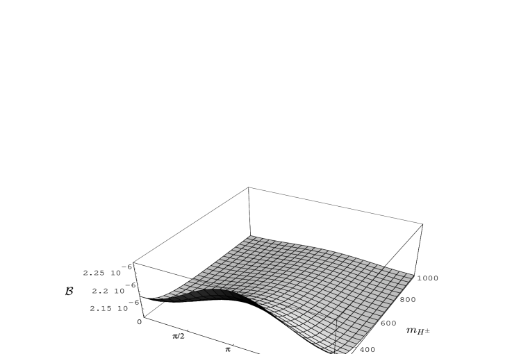
Figure 1:

Figure 2:

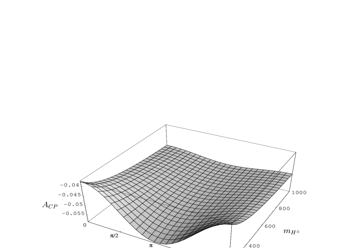
Figure 3: