Abstract

In the present paper we implement a non-trivial and renormalizable extension of the NJL model. We discuss the advantages and shortcomings of this extended model compared to a usual effective Pauli-Villars regularized version. We show that both versions become equivalent in the case of a large cutoff. Various relevant mesonic observables are calculated and compared.

ABSTRACT

1 Introduction

The Nambu and Jona-Lasinio (NJL) model [1] and its extensions have received much attention in low and medium energy hadronic physics [2, 3]. Because of its four fermion interaction it is non-renormalizable in the weak-coupling expansion for $d>2$ dimensions, the reason for the model usually being treated with a cutoff $\Lambda$ introduced to regularize the appearing ultraviolet (UV) divergencies. Although the original theory is non-renormalizable in perturbation theory, it becomes renormalizable in the mean-field expansion also for $d>2$ [4, 5, 7]. However, in contrast to $d<4$ where the NJL model represents a perfect renormalizable field theory it is supposed to collapse for $d=4$ to a trivial theory of non-interacting bosons [8, 9, 10]. Therefore in order to prevent the collapse, a cutoff $\Lambda$ has also to be retained in the ”renormalized” theory. The scale of this cutoff may in principle be deduced from an underlying non-trivial theory, in our case presumably QCD. If a finite $\Lambda$ could be chosen large enough to extend the integrations of all finite integrals to infinity, then the cutoff appears only implicitly within the couplings which are prevented from being driven to zero. Formally this may be achieved by augmenting the model by bosonic kinetic terms and quartic self-couplings, capable to absorb the cutoff dependence of the coupling constants. This procedure results in a renormalizable and non-trivial field theory for $d=4$ dimensions which corresponds to a linear sigma model with quarks [11], but with fixed bosonic self-couplings. In order to distinguish this model from the familiar cutoff or regularized NJL we will call it simply renormalized version in the following.

This non-trivial extension of the NJL is motivated by the observation that some observables related to finite integrals require an infinite or at least a very large cutoff, most prominent example being the anomalous pion decay $\pi^{0}\to\gamma\gamma$ [12]. Due to the underlying symmetries of the model, it is clear that only processes which are sensitive to large momenta are sizeably influenced. Therefore many low-energy quantities, especially of course those used to fix the parameters of the model as e.g. the pion mass, are essentially the same as in the regularized version.

The renormalized version has all the positive features known to renormalizable theories, but suffers from the occurrence of Landau ghosts, a well known problem related to Lagrangians without asymptotic freedom [5, 6].

A recent work [13] presents a renormalizable extension of the NJL-model by including the quark interaction generated by one gluon exchange, which simultaneously screens out the unphysical ghosts. The quark self-energy becomes momentum dependent with the appropriate asymptotic behavior, in contrast to the constant value obtained in the original NJL model. We consider our approach to be the ”minimal” non-trivial renormalization program which still keeps the simple local structure of the original NJL Lagrangian and we think it worthwhile to analyse the results obtained from this approach, due to its simplicity.

The aim of this paper is twofold. In the first part, which is of formal character, we show how to implement the original NJL Lagrangian to render it a non trivial renormalizable theory. Secondly we apply this Lagrangian to calculate relevant observables of the SU(2) flavor case and make a comparative study with the Pauli-Villars regularized version. We intend in this way to get a better understanding of the advantages and shortcomings of the two possible descriptions of the model in leading $1/N_{C}$ order.

2 Mean field expansion of the NJL model and triviality

In this section we briefly recapitulate the main features of the renormalization procedure for the NJL model using the mean-field expansion. Following Eguchi [4] we isolate the UV singularities, but we consider also finite contributions which enter the renormalization scheme in order to demonstrate the equivalence to the procedure presented by Guralnik and Tamvakis [5]. In addition we allow the symmetry to be broken explicitly by a current quark mass. Finally we discuss the issue of triviality and the introduction of a cutoff $\Lambda$ preventing the model from the collapse. The following derivation applies to SU(2) with $N_{C}$ colors, an extension to SU(3) is straightforward.

Starting point is the NJL Lagrangian with a local four-quark interaction

$$L=\bar{q}(i\gamma^{\mu}\partial_{\mu}-\hat{m}_{0})q+\frac{G_{0}}{2}\left[(\bar{q}q)^{2}+(\bar{q}i\gamma_{5}\mbox{\boldmath$\tau$}q)^{2}\right]\,,$$ (1)

where we consider the isospin symmetric limit $\hat{m}_{u}=\hat{m}_{d}=\hat{m}$. To allow for wave function renormalizations later on and also in order to trace the $N_{C}$ orders, it is convenient to replace $G_{0}=g_{0}^{2}/\mu_{0}^{2}$ with $g_{0}^{2}\sim 1/N_{C}$. The subscript zero denotes bare (infinite) quantities everywhere. With boson fields introduced in the standard way the Lagrangian becomes

$$L = \bar{q}\left[i\gamma^{\mu}\partial_{\mu}-\hat{m}_{0}-g_{0}(\sigma_{0}+i\gamma_{5}\mbox{\boldmath$\tau\pi$}_{0})\right]q-\frac{\mu^{2}_{0}}{2}(\sigma_{0}^{2}+\mbox{\boldmath$\pi$}_{0}^{2})$$ (2)

$$L = \bar{q}\left[i\gamma^{\mu}\partial_{\mu}-g_{0}(\sigma_{0}+i\gamma_{5}\mbox{\boldmath$\tau\pi$}_{0})\right]q-\frac{\mu^{2}_{0}}{2}(\sigma_{0}^{2}+\mbox{\boldmath$\pi$}_{0}^{2})+\frac{\mu_{0}^{2}}{g_{0}}\hat{m}_{0}\sigma_{0}\,,$$ (3)

where the latter representation is obtained by shifting the scalar field $\sigma_{0}\to\sigma_{0}-\hat{m}_{0}/g_{0}$ and a term independent of the dynamical fields is omitted. Integrations over the fermion fields $q$ and $\bar{q}$ may now be performed in the path integral such that the resulting effective Lagrangian collects the corresponding trace log contribution

$$L=-iTr\ell n\left[i\gamma^{\mu}\partial_{\mu}-g_{0}(\sigma_{0}+i\gamma_{5}\mbox{\boldmath$\tau\pi$}_{0})\right]-\frac{\mu^{2}_{0}}{2}(\sigma_{0}^{2}+\mbox{\boldmath$\pi$}_{0}^{2})+\frac{\mu_{0}^{2}}{g_{0}}\hat{m}_{0}\sigma_{0}\,.$$ (4)

Expecting the scalar field to possess a nonvanishing vacuum expectation value we expand $\sigma_{0}=m/g_{0}+\sigma_{0}^{\prime}$, where $m$ represents the (finite) constituent mass

$$L=i\sum_{n=1}^{\infty}\frac{1}{n}Tr\left[(i\gamma^{\mu}\partial_{\mu}-m)^{-1}g_{0}(\sigma_{0}^{\prime}+i\gamma_{5}\mbox{\boldmath$\tau\pi$}_{0})\right]^{n}-\frac{\mu^{2}_{0}}{2}(\sigma_{0}^{\prime 2}+\mbox{\boldmath$\pi$}_{0}^{2})-\frac{\mu_{0}^{2}}{g_{0}}(m-\hat{m}_{0})\sigma_{0}^{\prime}\,.$$ (5)

To evaluate this sum is now quite straightforward. The terms for $n=1,\dots,4$ contain UV divergencies showing up as

$$I_{quad}=i\int\frac{d^{4}q}{(2\pi)^{4}}\frac{1}{q^{2}-m^{2}}\,,\qquad I_{log}=i\int\frac{d^{4}q}{(2\pi)^{4}}\frac{1}{(q^{2}-m^{2})^{2}}$$ (6)

quadratically and logarithmically divergent integrals respectively. The effective Lagrangian is then given by

$$L = \frac{1}{2}(-4N_{C}g_{0}^{2}I_{log})(\partial_{\mu}\sigma_{0}^{\prime}\partial^{\mu}\sigma_{0}^{\prime}+\partial_{\mu}\mbox{\boldmath$\pi$}_{0}\partial^{\mu}\mbox{\boldmath$\pi$}_{0})-\frac{N_{C}g_{0}^{2}}{12\pi^{2}}\partial_{\mu}\sigma_{0}^{\prime}\partial^{\mu}\sigma_{0}^{\prime}$$ (10)

$$-\frac{1}{2}(\mu_{0}^{2}-8N_{C}g_{0}^{2}I_{quad})(\sigma_{0}^{\prime 2}+\mbox{\boldmath$\pi$}_{0}^{2})-\frac{1}{2}4m^{2}(-4N_{C}g_{0}^{2}I_{log})\sigma_{0}^{\prime 2}+\dots$$

$$+8N_{C}g_{0}^{3}I_{log}m\sigma_{0}^{\prime}(\sigma_{0}^{\prime 2}+\mbox{\boldmath$\pi$}_{0}^{2})+2N_{C}g_{0}^{4}I_{log}(\sigma_{0}^{\prime 2}+\mbox{\boldmath$\pi$}_{0}^{2})^{2}+\dots$$

$$-\left[\frac{\mu_{0}^{2}}{g_{0}}(m-\hat{m}_{0})-8N_{C}g_{0}mI_{quad}\right]\sigma_{0}^{\prime}\,.$$

The dots after the first two lines denote finite higher derivative terms of $g_{0}^{2}\sigma_{0}^{2}$ and $g_{0}^{2}\mbox{\boldmath$\pi$}_{0}^{2}$ proportional to $N_{C}^{0}$ not explicitely shown, but a finite kinetic term for the scalars is kept and finally leads to different wave-function renormalizations $\sigma^{\prime}=Z_{\sigma}^{-1/2}\sigma_{0}^{\prime}$ and $\mbox{\boldmath$\pi$}=Z_{\pi}^{-1/2}\mbox{\boldmath$\pi$}_{0}$. The dots in the third line indicate finite higher order terms also not shown. The renormalized parameters may now be introduced as follows

$$Z_{\sigma}^{-1}=\frac{g_{0}^{2}}{g_{\sigma}^{2}}=-4N_{C}g_{0}^{2}I_{log}-\frac{N_{C}g_{0}^{2}}{6\pi^{2}}$$ (11)

$$Z_{\pi}^{-1}=\frac{g_{0}^{2}}{g_{\pi}^{2}}=-4N_{C}g_{0}^{2}I_{log}$$ (12)

$$\frac{\mu^{2}_{\sigma}}{Z_{\sigma}}=\mu_{0}^{2}-8N_{C}g_{0}^{2}(I_{quad}+2m^{2}I_{log})$$ (13)

$$\frac{\mu^{2}_{\pi}}{Z_{\pi}}=\mu_{0}^{2}-8N_{C}g_{0}^{2}I_{quad}\,.$$ (14)

Together with the gap-equation

$$\frac{\mu_{0}^{2}}{g_{0}^{2}}(m-\hat{m}_{0})=8N_{C}mI_{quad}\,,$$ (15)

which makes the linear term in $\sigma_{0}^{\prime}$ vanish, we obtain the renormalized Lagrangian in its final form

$$L = \frac{1}{2}(\partial_{\mu}\sigma^{\prime}\partial^{\mu}\sigma^{\prime}+\partial_{\mu}\mbox{\boldmath$\pi$}\partial^{\mu}\mbox{\boldmath$\pi$})-\frac{1}{2}(\mu_{\sigma}^{2}\sigma^{\prime 2}+\mu_{\pi}^{2}\mbox{\boldmath$\pi$}^{2})$$ (17)

$$-\frac{2mg_{\sigma}}{g_{\pi}^{2}}\sigma^{\prime}(g_{\sigma}^{2}\sigma^{\prime 2}+g_{\pi}^{2}\mbox{\boldmath$\pi$}^{2})-\frac{1}{2g_{\pi}^{2}}(g_{\sigma}^{2}\sigma^{\prime 2}+g_{\pi}^{2}\mbox{\boldmath$\pi$}^{2})^{2}\,+\dots$$

The current quark mass has disappeared and it is noticed that the remaining parameters are related according to eqs. (7-10)

$$\frac{1}{g_{\sigma}^{2}}=\frac{1}{g_{\pi}^{2}}-\frac{N_{C}}{6\pi^{2}}\,,\qquad\quad\frac{\mu_{\sigma}^{2}}{g_{\sigma}^{2}}=\frac{4m^{2}+\mu_{\pi}^{2}}{g_{\pi}^{2}}$$ (18)

such that the renormalized model is characterized by three parameters ($m,g_{\pi},\mu_{\pi}$) as the regularized one ($G,m,\hat{m}$). From these equations using the gap-equation (15) we may also define a renormalized four-fermion coupling $G$

$$m\frac{\mu_{\pi}^{2}}{g_{\pi}^{2}}=\hat{m}_{0}\frac{\mu_{0}^{2}}{g_{0}^{2}}=\frac{\hat{m}_{0}}{G_{0}}=\frac{\hat{m}}{G}$$ (19)

by reintroduction of the renormalized (physical) current quark mass. Although this relation is beyond the scope of the renormalized model it will nevertheless prove useful for the evaluation of the quark condensate.

The $N_{C}$ orders are now carried by the couplings $g_{\pi}^{2}\sim g_{\sigma}^{2}\sim 1/N_{C}$. For practical calculations we consider only the leading order $N_{C}$ for each process. From the quadratic terms in the Lagrangian we read off the renormalized meson propagators of order $N_{C}^{0}$

$$\Delta_{\sigma}^{-1}(p^{2})=p^{2}-\mu_{\sigma}^{2}-4N_{C}g_{\sigma}^{2}\left[(p^{2}-4m^{2})Z_{0}(p^{2})-\frac{p^{2}}{24\pi^{2}}\right]$$ (20)

$$\Delta_{\pi}^{-1}(p^{2})=p^{2}-\mu_{\pi}^{2}-4N_{C}g_{\pi}^{2}p^{2}Z_{0}(p^{2})\,,$$ (21)

where the momentum dependent terms due to the finite higher derivative terms not explicitely shown in eq.(17) are contained in the finite function

$$Z_{0}(p^{2}) = \frac{1}{16\pi^{2}}\int_{0}^{1}dz\ell n\left[1-\frac{p^{2}}{m^{2}}z(1-z)\right]$$ (22)

$$= \frac{1}{8\pi^{2}}\left\{\begin{array}[]{ll}\sqrt{1+\frac{4m^{2}}{|p^{2}|}}\mbox{arsinh}\sqrt{\frac{|p^{2}|}{4m^{2}}}-1&\qquad\qquad\qquad p^{2}\leq 0\\ \sqrt{\frac{4m^{2}}{p^{2}}-1}\arcsin{\sqrt{\frac{p^{2}}{4m^{2}}}}-1&\qquad\qquad 0<p^{2}\leq 4m^{2}\\ \sqrt{1-\frac{4m^{2}}{p^{2}}}\left(\mbox{arcosh}\sqrt{\frac{p^{2}}{4m^{2}}}-i\frac{\pi}{2}\right)-1&\;\qquad\enspace 4m^{2}<p^{2}\\ \end{array}\right.$$ (27)

which possesses different branches. The physical meson masses are defined as usual via the poles of the propagators

$$m_{\sigma}^{2}=4m^{2}+\mu_{\pi}^{2}+4N_{C}g_{\pi}^{2}(m_{\sigma}^{2}-4m^{2})Z_{0}(m_{\sigma}^{2})$$ (28)

$$m_{\pi}^{2}=\mu_{\pi}^{2}+4N_{C}g_{\pi}^{2}m_{\pi}^{2}Z_{0}(m_{\pi}^{2})\,.$$ (29)

In the chiral limit ($\mu_{\pi}^{2}=0$) we obtain $m_{\pi}=0$ and $m_{\sigma}=2m$.

Similarly, also in the chiral limit the leading $N_{C}$ 3- and 4-boson vertex functions at zero momenta are obtained from the cubic and quartic self-couplings in accordance with Guralnik and Tamvakis [5], who derive these results from the corresponding Ward identities.

In the following we want to discuss the triviality of the NJL model which is suggested by lattice calculations [10]. In the mean-field expansion it follows immediately from (8)

$$g_{\pi}^{2}=-(4N_{C}I_{log})^{-1}\,,$$ (30)

namely in the continuum limit the couplings $g_{\pi}$ and hence also $g_{\sigma}$ are driven to zero rendering the Lagrangian (17) a theory of non-interacting mesons. This is caused by the mesonic kinetic terms and quartic self couplings in (17) being created purely by radiative corrections: they were not present in the original Lagrangian. To avoid the collapse of the model, $g_{\pi}$ must be kept fixed at some finite value. For that purpose a cutoff $\Lambda$ has to be introduced in order to keep the logarithmically divergent integral in (30) finite (note that the quadratic divergence has already disappeared in the renormalized parameters). In the continuum limit $g_{\pi}^{2}\sim(4\pi/N_{C})/\ell n(\Lambda/m)$ tends to zero logarithmically, and a finite coupling $g_{\pi}$ requires also a finite $\Lambda$, in fact, in order to reproduce a reasonable coupling strength a rather low cutoff of the order of $1$GeV is needed in contrast to the situation in QED where the collaps is prevented by a cutoff located way above all physical energies of interest. Nevertheless, if it were possible to choose $\Lambda$ large enough such that all finite integrals may be evaluated in the continuum limit then the cutoff would disappear from the theory being only implicitely contained in the coupling $g_{\pi}$ which is kept finite [14]. Exactly this is achieved by adding mesonic kinetic terms and quartic self-couplings to the model which are capable to absorb the troublesome radiative terms in (17) leading to a non-trivial renormalizable extension of the NJL discussed in the following section. Mesonic properties calculated in the two versions of the model are then presented in section 4.

3 Non-trivial extension of the NJL model

We have seen in the previous section that the triviality of the NJL model is connected with the fact that the mesonic kinetic and interaction terms are created purely by radiative corrections. In fact triviality may be avoided by adding these contributions to the Lagrangian (4) from the beginning [15]

$$L = -iTr\ell n\left[i\gamma^{\mu}\partial_{\mu}-g_{0}(\sigma_{0}+i\gamma_{5}\mbox{\boldmath$\tau\pi$}_{0})\right]+\frac{f_{0}^{2}}{2}(\partial_{\mu}\sigma_{0}\partial^{\mu}\sigma_{0}+\partial_{\mu}\mbox{\boldmath$\pi$}_{0}\partial^{\mu}\mbox{\boldmath$\pi$}_{0})$$ (32)

$$-\frac{\mu^{2}_{0}}{2}(\sigma_{0}^{2}+\mbox{\boldmath$\pi$}_{0}^{2})-\frac{\lambda_{0}}{2}(\sigma_{0}^{2}+\mbox{\boldmath$\pi$}_{0}^{2})^{2}+\frac{\mu_{0}^{2}}{g_{0}}\hat{m}_{0}\sigma_{0}+\dots$$

Of course this may lead beyond the NJL model, we will comment on this later. Repeating the steps which lead to eq. (10) we find the renormalized parameters as

$$Z_{\sigma}^{-1}=\frac{g_{0}^{2}}{g_{\sigma}^{2}}=f_{0}^{2}-4N_{C}g_{0}^{2}I_{log}-\frac{N_{C}g_{0}^{2}}{6\pi^{2}}$$ (33)

$$Z_{\pi}^{-1}=\frac{g_{0}^{2}}{g_{\pi}^{2}}=f_{0}^{2}-4N_{C}g_{0}^{2}I_{log}$$ (34)

$$\frac{\mu^{2}_{\sigma}}{Z_{\sigma}}=\mu_{0}^{2}-8N_{C}g_{0}^{2}(I_{quad}+2m^{2}I_{log})+\frac{6\lambda_{0}}{g_{0}^{2}}m^{2}$$ (35)

$$\frac{\mu^{2}_{\pi}}{Z_{\pi}}=\mu_{0}^{2}-8N_{C}g_{0}^{2}I_{quad}+\frac{2\lambda_{0}}{g_{0}^{2}}m^{2}$$ (36)

$$\frac{\lambda}{g_{\pi}^{2}}=\frac{\lambda_{0}}{g_{0}^{4}}-4N_{C}I_{log}$$ (37)

together with the gap-equation

$$\frac{\mu_{0}^{2}}{g_{0}^{2}}(m-\hat{m}_{0})-8N_{C}mI_{quad}+\frac{2\lambda_{0}}{g_{0}^{4}}m^{3}=0\,.$$ (38)

The renormalized Lagrangian in the shifted scalar fields becomes

$$L = \frac{1}{2}(\partial_{\mu}\sigma^{\prime}\partial^{\mu}\sigma^{\prime}+\partial_{\mu}\mbox{\boldmath$\pi$}\partial^{\mu}\mbox{\boldmath$\pi$})-\frac{1}{2}(\mu_{\sigma}^{2}\sigma^{\prime 2}+\mu_{\pi}^{2}\mbox{\boldmath$\pi$}^{2})$$ (40)

$$-\frac{2m\lambda}{g_{\pi}^{2}}g_{\sigma}\sigma^{\prime}(g_{\sigma}^{2}\sigma^{\prime 2}+g_{\pi}^{2}\mbox{\boldmath$\pi$}^{2})-\frac{\lambda}{2g_{\pi}^{2}}(g_{\sigma}^{2}\sigma^{\prime 2}+g_{\pi}^{2}\mbox{\boldmath$\pi$}^{2})^{2}\,+\dots$$

formally identical to the bosonized NJL Lagrangian (17) if we choose $\lambda=1$. In general the model parameters are now related

$$\frac{1}{g_{\sigma}^{2}}=\frac{1}{g_{\pi}^{2}}-\frac{N_{C}}{6\pi^{2}}\,,\qquad\quad\frac{\mu_{\sigma}^{2}}{g_{\sigma}^{2}}=\frac{4\lambda m^{2}+\mu_{\pi}^{2}}{g_{\pi}^{2}}$$ (41)

quite similar to (18) and also the relation (19) remains unchanged. We want to emphasize however, that this Lagrangian does not represent the trivial NJL model and constitutes instead a different non-trivial theory. As a consequence the couplings $g_{\pi}$ and $g_{\sigma}$ do no longer vanish in the continuum limit. The numerical results of this model with $\lambda=1$ are of course identical to those obtained from the NJL model (17) with $g_{\pi}$ and $g_{\sigma}$ kept fixed at some finite values as discussed in the preceeding section.

Concluding, there seems to be two options to treat the problem of triviality which appears in the NJL model:

• A cutoff $\Lambda$ is retained to prevent the model from the collapse. Because numerically the cutoff is of the order of $1$ GeV only, it has to be kept also in all finite integrals.

• The NJL model is augmented by kinetic terms and mesonic self-interactions. This results in the linear sigma model coupled to quarks and constitutes a perfect non-trivial field theory.

The latter theory contains one additional parameter $\lambda$. For $\lambda=1$ (ii) gives the same results as the conventional NJL in case of a large cutoff. In principle the assumption $\lambda=1$ may be tested in $\pi\pi$ scattering, of course not in the leading chiral order which is fixed by a famous low energy theorem [16], but in the next to leading orders (subsection 4.2). Many other meson properties are quite independent of this parameter. In the following section we compare some mesonic observables calculated in the two versions of the NJL model.

4 Meson properties

In this section the parameters of both versions of the model are fixed. We show that in the renormalized version the chiral expansion becomes quite simple and we discuss the issue of the additional parameter $\lambda$ appearing in the linear sigma model with quarks. Finally we are going to calculate several mesonic observables.

1 Determination of the model parameters

For both versions of the model we used two sets of model parameters : one with a low constituent quark mass fixed at $m=210$ MeV, and the other with the constituent quark mass fixed at $m=350$ MeV, values which are used widely in the literature. The remaining model parameters are adjusted to reproduce the pion decay constant $f_{\pi}=93.3$ MeV and the pion mass $m_{\pi}=139$ MeV. As a result, one obtains for the Pauli-Villars regularized version a large dimensionless ratio $\Lambda/m\simeq 6$ in the small constituent quark mass case, and a small one for the large mass case, $\Lambda/m\simeq 2$, see Table I. As will be discussed in section 4.2, chiral expansions of the renormalized and regularized versions coincide in the $\Lambda/m\to\infty$ limit, showing that this ratio is a measure for the deviations in the two models. On the other hand, in the renormalized version the pion decay constant is

$$f_{\pi}=g_{\pi qq}\frac{m}{g_{\pi}^{2}}\frac{\mu_{\pi}^{2}}{m_{\pi}^{2}}\,,$$ (42)

and the pion mass is given by (28). Here and in the following we use the pion quark and sigma quark couplings

$$g_{\pi qq}^{-2}=g_{\pi}^{-2}-4N_{C}\left[Z_{0}(m_{\pi}^{2})+m_{\pi}^{2}Z_{0}^{\prime}(m_{\pi}^{2})\right]$$ (43)

$$g_{\sigma qq}^{-2}=g_{\pi}^{-2}-4N_{C}\left[Z_{0}(m_{\sigma}^{2})+(m_{\sigma}^{2}-4m^{2})Z_{0}^{\prime}(m_{\sigma}^{2})\right]\,,$$ (44)

for abbreviation. Thus, $f_{\pi}$ and $m_{\pi}$ fix the parameters $g_{\pi}$ and $\mu_{\pi}$ listed also in Table I. Furthermore, for the evaluation of the quark condensate according to (19)

$$\hat{m}<\bar{q}q>=-(m-\hat{m})\frac{\hat{m}}{G}=-m(m-\hat{m})\frac{\mu_{\pi}^{2}}{g_{\pi}^{2}}$$ (45)

a value for the current quark mass has to be adopted which strictly speaking is not a parameter of the renormalized version of the model. The standard value of $\hat{m}=7.5$ MeV leads to the result quoted in Table II.

TABLE I.: Parameters of the regularized and renormalized versions of the NJL model.

	regularized	model		renormalized	model
model	$m=350$	($210$)	MeV	$m=350$	($210$)	MeV
parameters	$G=17.6$	($5.11$)	GeV-2	$g_{\pi}=3.752$	($2.250$)
	$\hat{m}=8.5$	($4.1$)	MeV	$\mu_{\pi}=141$	($141$)	MeV
related	$\Lambda=769$	($1190$)	MeV	$g_{\sigma}=7.006$	($2.610$)
parameters				$\mu_{\sigma}=1333$	($513.8$)	MeV

2 Chiral expansion and $\pi\pi$ scattering

In the renormalized version of the NJL model the chiral expansion for constituent quark mass, pion decay constant, pion mass and quark condensate become quite simple:

$$m={\stackrel{{\scriptstyle\circ}}{{m}}}\left[1+\frac{{\stackrel{{\scriptstyle\circ}}{{m}}}_{\pi}^{2}}{4{\stackrel{{\scriptstyle\circ}}{{m}}}^{2}}+\dots\right]$$ (46)

$$f_{\pi}^{2}={\stackrel{{\scriptstyle\circ}}{{f}}}_{\pi}^{2}\left[1+\frac{{\stackrel{{\scriptstyle\circ}}{{m}}}_{\pi}^{2}}{2{\stackrel{{\scriptstyle\circ}}{{m}}}^{2}}-\frac{N_{C}{\stackrel{{\scriptstyle\circ}}{{m}}}_{\pi}^{2}}{8\pi^{2}{\stackrel{{\scriptstyle\circ}}{{f}}}_{\pi}^{2}}+\dots\right]$$ (47)

$$m_{\pi}^{2}={\stackrel{{\scriptstyle\circ}}{{m}}}_{\pi}^{2}\left[1-\frac{{\stackrel{{\scriptstyle\circ}}{{m}}}_{\pi}^{2}}{4{\stackrel{{\scriptstyle\circ}}{{m}}}^{2}}+\frac{N_{C}{\stackrel{{\scriptstyle\circ}}{{m}}}_{\pi}^{2}}{12\pi^{2}{\stackrel{{\scriptstyle\circ}}{{f}}}_{\pi}^{2}}+\dots\right]$$ (48)

$$\hat{m}<\bar{q}q>=-{\stackrel{{\scriptstyle\circ}}{{f}}}_{\pi}^{2}{\stackrel{{\scriptstyle\circ}}{{m}}}_{\pi}^{2}\left[1-\frac{\hat{m}}{{\stackrel{{\scriptstyle\circ}}{{m}}}}+\frac{{\stackrel{{\scriptstyle\circ}}{{m}}}_{\pi}^{2}}{4{\stackrel{{\scriptstyle\circ}}{{m}}}^{2}}+\dots\right]\,.$$ (49)

These formulas agree with those obtained in the Pauli-Villars regularized model [17] for large cutoff $\Lambda\gg m$. It is noticed that the current quark mass appears only in the expression for the condensate.

Similarly, the $\pi\pi$ scattering amplitude (box-diagram + sigma exchange) is obtained as

$$A(s,t,u) = \frac{s-{\stackrel{{\scriptstyle\circ}}{{m}}}_{\pi}^{2}}{{\stackrel{{\scriptstyle\circ}}{{f}}}_{\pi}^{2}}+\left[1-\frac{N_{C}{\stackrel{{\scriptstyle\circ}}{{m}}}^{2}}{3\pi^{2}{\stackrel{{\scriptstyle\circ}}{{f}}}_{\pi}^{2}}+\frac{N_{C}^{2}{\stackrel{{\scriptstyle\circ}}{{m}}}^{4}}{16\pi^{4}{\stackrel{{\scriptstyle\circ}}{{f}}}_{\pi}^{4}}\right]\frac{\left(s-2{\stackrel{{\scriptstyle\circ}}{{m}}}_{\pi}^{2}\right)^{2}}{4{\stackrel{{\scriptstyle\circ}}{{m}}}^{2}{\stackrel{{\scriptstyle\circ}}{{f}}}_{\pi}^{2}}$$ (52)

$$+(\frac{1}{\lambda}-1)\frac{1}{4{\stackrel{{\scriptstyle\circ}}{{m}}}^{2}{\stackrel{{\scriptstyle\circ}}{{f}}}_{\pi}^{2}}\left[s-{\stackrel{{\scriptstyle\circ}}{{m}}}_{\pi}^{2}-\frac{N_{C}{\stackrel{{\scriptstyle\circ}}{{m}}}^{2}}{4\pi^{2}{\stackrel{{\scriptstyle\circ}}{{f}}}_{\pi}^{2}}\left(s-2{\stackrel{{\scriptstyle\circ}}{{m}}}_{\pi}^{2}\right)\right]^{2}$$

$$+\frac{N_{C}}{24\pi^{2}{\stackrel{{\scriptstyle\circ}}{{f}}}_{\pi}^{4}}\left[s(u+t)-ut-2{\stackrel{{\scriptstyle\circ}}{{m}}}_{\pi}^{4}\right]+\dots$$

As mentioned already, the leading term is fixed by a low energy theorem [16] and is therefore independent of the strength $\lambda$ of the quartic self-interaction. However, in the next to leading order there appears a term in addition to those obtained in the regularized model [17] with large cutoff, which is effective for $\lambda\not=1$.

In refs.[17, 3] it was shown that compatibility with chiral perturbation theory (ChPT) requires a small constituent quark mass of the order of $m\simeq 250$ MeV. For such a small quark mass the cutoff is of minor importance and the terms in (52) which survive for $\lambda=1$ fit the ChPT $\pi\pi$ scattering threshold parameters [18] in the renormalized version as well. We may conclude that the comparison with ChPT requires a value of $\lambda$ close to $1$. Of course, this conclusion is correct only if we accept a small constituent quark mass.

3 Sigma meson properties

The sigma meson mass can be evaluated using eq.(28). In order to obtain this mass, we made use of the real part of the propagator only, in both, the regularized and the renormalized version. The imaginary part related to the decays into $\bar{q}q$ pairs is very small and can be neglected [19]. The decay width of $\sigma\to\pi\pi$ is :

$$\Gamma_{\sigma\pi\pi}=\frac{3\sqrt{m_{\sigma}^{2}-4m_{\pi}^{2}}}{8\pi m_{\sigma}^{2}}f_{\sigma\pi\pi}^{2}\,.$$ (53)

All the expressions for the Pauli-Villars regularized NJL model used here and in the following sections may be found in [20] and are not repeated here. The amplitude $f_{\sigma\pi\pi}$ reads in the renormalized version

$$f_{\sigma\pi\pi}=16mN_{C}g_{\sigma qq}g_{\pi qq}^{2}\left[\frac{1}{4N_{C}g_{\pi}^{2}}-Z_{0}(m_{\sigma}^{2})+\frac{2m_{\pi}^{2}-m_{\sigma}^{2}}{2}I_{3}(m_{\sigma}^{2},m_{\pi}^{2},m_{\pi}^{2})\right]\,,$$ (54)

$$I_{3}(p^{2},p_{1}^{2},p_{2}^{2})=i\int{\frac{d^{4}q}{(2\pi)^{4}}\frac{1}{(q^{2}-m^{2})[(q-p_{1})^{2}-m^{2}][(q-p_{2})^{2}-m^{2}]}}$$ (55)

with $p^{2}=(p_{1}-p_{2})^{2}$.

As is noticed from Table II, the scalar decay width into two pions depends most sensitively on the two versions of the model, specially of course in the large mass (low cutoff) case. This difference persists also in the chiral limit.

4 Pion charge formfactor

In the renormalized version, the pion electromagnetic formfactor is given by

$$F_{\pi}(p^{2})=2N_{C}g_{\pi qq}^{2}\left[\frac{1}{4N_{C}g_{\pi}^{2}}+m_{\pi}^{2}\left(Z_{0}^{\prime}(m_{\pi}^{2})-I_{3}(p^{2},m_{\pi}^{2},m_{\pi}^{2})\right)\right]\,,$$ (56)

and the corresponding pion electromagnetic radius is defined as usual. In Fig. 1 the electromagnetic pion formfactor is shown in the space-like region only, since in the time-like region the role of vector mesons, which are not considered here, is very important. For the same reason the charge radius turns out too small compared to its experimental value, see Table II. We see however that the renormalizable version yields a value close to the chiral limit result

$$<r^{2}>_{\pi}=\frac{3N_{C}}{4\pi^{2}f_{\pi}^{2}}\simeq(0.59fm)^{2}\,,$$ (57)

whereas the regularized version tends to decrease this value further with decreasing ratio $\Lambda/m$. From Fig.1 we see that the formfactors in the two versions of the model are very similar for the lower mass case, but for the larger mass case the renormalized version improves on the results, whereas the regularized version does not yield a satisfactory fit as noticed already in [12].

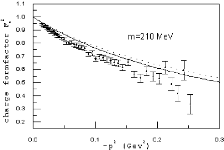
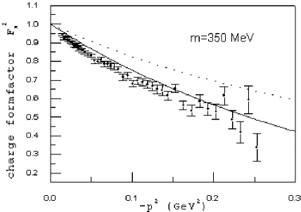
FIG. 1.: Pion formfactor in the space-like region. The results of the renormalized (solid) and regularized (dashed) models for small and large constituent quark masses are compared to experimental data [21].

5 Anomalous $\pi^{0}\to\gamma\gamma$ decay

The formfactor associated with the anomalous process $\pi_{0}\to\gamma^{*}\gamma$, with one of the photons being off shell is

$$F_{\pi\gamma^{*}\gamma}(p^{2})=-\frac{8N_{C}e^{2}}{3}g_{\pi qq}mI_{3}(0,p^{2},m^{2}_{\pi})\,.$$ (58)

With both photons on-shell one obtains the anomalous pion decay $\pi_{0}\to\gamma\gamma$ analytically in the renormalized version, given by the following expression:

$$\Gamma_{\pi^{0}\to\gamma\gamma}=\frac{m_{\pi^{0}}^{3}}{64\pi}F_{\pi\gamma\gamma}^{2}\,,\qquad F_{\pi\gamma\gamma}=-\frac{N_{C}e^{2}g_{\pi qq}}{3\pi^{2}m_{\pi}}\frac{m}{\sqrt{4m^{2}-m_{\pi}^{2}}}\arctan\frac{m_{\pi}}{\sqrt{4m^{2}-m_{\pi}^{2}}}\,.$$ (59)

In the chiral limit, this reduces to the well-known result [22]

$$\Gamma_{\pi^{0}\to\gamma\gamma}=\frac{m_{\pi^{0}}^{3}}{64\pi}\left(\frac{N_{C}e^{2}}{12\pi^{2}f_{\pi}}\right)^{2}\,.$$ (60)

The model independent amplitude for the anomalous $\pi^{0}\to\gamma\gamma$ decay in the chiral limit is obtained exactly only in the renormalized version. The regularized version renders the decay width strongly cutoff dependent (see Table II). This formal result is one of the obvious advantages of the renormalized model. In this context we should mention that in the spirit of regularized models a consistent treatment of anomalous processes has been forwarded in [23], where the quark-loop is regulated dynamically by the intrinsic non-locality of the quark-meson interaction.

The $\pi^{0}\to\gamma^{*}\gamma$ transition formfactor as it is obtained in the renormalized version is plotted in Fig.2. We do not compare to the results of the regularized version, because it fails already at the photon point (Table II). Obviously here the lower mass case leads to a much better fit to experiment. The slope of the formfactor at the origin is obtained as $a_{\pi^{0}}=0.035m^{2}_{\pi^{0}}$ which has to be compared to the empirical value $a_{\pi^{0}}=0.0326\pm 0.0026m^{2}_{\pi^{0}}$, [24].

TABLE II.: Some meson properties calculated in the regularized and renormalized versions of the NJL model are compared to experimental data [25, 26]. The asterisks indicate quantities which served as input to determine the model parameters. Results are calculated for a constituent quark mass of $m=350$ MeV and $m=210$ MeV (in brakets).

		regularized	model	renormalized	model	experiment
$f_{\pi}$	[MeV]	$93.3^{*}$		$93.3^{*}$		$93.3$
$m_{\pi}$	[MeV]	$139^{*}$		$139^{*}$		$139$
$m_{\sigma}$	[MeV]	$705$	($434$)	$705$	($433$)	$\sim 700$
$\Gamma_{\sigma\to\pi\pi}$	[MeV]	$647$	($336$)	$457$	($307$)	$\sim 700$
$\Gamma_{\pi^{0}\to\gamma\gamma}$	[eV]	$3.7$	($7.2$)	$7.6$	($8.3$)	$7.7\pm 0.6$
$<r^{2}>_{\pi}^{1/2}$	[fm]	$0.49$	($0.59$)	$0.58$	($0.59$)	$0.678\pm 0.012$
$<\bar{q}q>$	[MeV3]	$-265^{3}$	($-340^{3}$)	$-283^{3}$	($-281^{3}$)	$-(270\pm 20)^{3}$

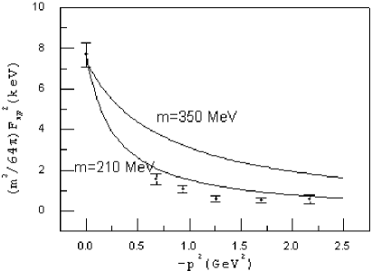
FIG. 2.: Transition formfactor for the anomalous process $\pi^{0}\to\gamma^{*}\gamma$ in the space-like region as calculated in the renormalized version with different constituent quark masses. The data are from Ref. [24].

For the larger $\Lambda/m$ ratio the results in Table II are quite similar in the two versions as expected. For the larger constituent mass case, however, the results for the anomalous pion decay and the pion electromagnetic radius are substantially improved in the renormalized version.

5 Conclusions

We have considered a non-trivial and renormalizable extension of the NJL model obtained by adding the necessary counter terms, namely the mesonic kinetic energies and quartic mesonic interactions to the originial Lagrangian. This amounts to a linear sigma model coupled to quarks with fixed strength of the quartic mesonic self-interactions. It was shown that this version of the model coincides with its familiar regularized versions provided the cutoff is large enough.

We presented a comparative and quantitative analysis of the most relevant mesonic observables with an effective Pauli-Villars regularized version in leading $1/N_{C}$ order. We found that in the renormalized version of the model the electromagnetic pion decay is always (independently of other parameters) in agreement with experiment in contrast to results obtained in regularized versions (usually $\geq 30\%$ off). For the first time a reasonable description of the corresponding transition formfactor is obtained. In the regularized versions the quality of the results depends crucially on the ratio $\Lambda/m$ where $\Lambda$ is the four-dimensional cutoff and $m$ is the constituent quark mass. The larger the ratio, the better the agreement with phenomenology. This is in a way reflected in the renormalized version, where the agreement is systematically better when compared with the regularized version for the same $m$ value. We noticed that the quantitative results become quite similar in the two versions for ratios $\Lambda/m\stackrel{{\scriptstyle>}}{{{}_{\sim}}}6$.

Further applications of the extended non-trivial and renormalizable NJL model are the study of the SU(3) flavor case and the inclusion of vectors and axialvectors mesons. One of the most interesting issues related to the SU(3) sector is connected with the kaon decay constant which persistently turns out to be too small ($f_{K}\simeq f_{\pi}$) unless one is willing to accept a small nonstrange constituent quark mass of the order $m\simeq 210$MeV which brings along its own difficulties (small scalar meson masses, low $\bar{q}q$ threshold, etc.). Unfortunately the renormalizable version presented here is not capable to resolve this problem, the solution has to be sought elsewhere.

We are grateful to O. A. Battistel for critical remarks on regularization prescriptions [27]. H.W. would like to thank G. Holzwarth for clarifying comments on the renormalization of the model. The present research has been supported partly by JNICT, Portugal (Contract PRAXIS/4/4.1/BCC/2753 and PCERN/S/FIS/1162/97) and by CNPq-Brazil.

REFERENCES

• [1] Y. Nambu and G. Jona-Lasinio, Phys. Rev. 122 (1961) 345.
• [2] T. Hatsuda and T. Kunihiro, Phys. Rep. 247 (1994) 221.
• [3] J. Bijnens, Phys. Rep. 265 (1996) 369.
• [4] T. Eguchi, Phys. Rev. D14 (1976) 2755.
• [5] G.S.Guralnik and K. Tamvakis, Nucl. Phys. B148 (1979) 283.
• [6] R.J. Perry, Phys. Lett. B199 (1987) 489; R.J. Furnstal and C. Horowitz, Nucl. Phys. A485 (1988) 632.
• [7] B. Rosenstein, B.J. Warr and S.H. Park, Phys. Rev. Lett. 62 (1989) 1433.
• [8] K.G. Wilson, Phys. Rev. D7 (1973) 2911.
• [9] T. Eguchi, Phys. Rev. D17 (1978) 611.
• [10] S. Kim, A. Kocić and J. Kogut, Nucl. Phys. B429 (1994) 407.
• [11] J.-L. Gervais and B.W. Lee, Nucl. Phys. B12 (1969) 627.
• [12] A.H. Blin, B. Hiller and M. Schaden, Z. Phys. A331 (1988) 75.
• [13] K. Langfeld, C. Kettner and H. Reinhardt, Nucl. Phys. A608 (1996) 331.
• [14] S. Kawati and H. Miyata, Phys. Rev. D23 (1981) 3010.
• [15] S. Weinberg, Phys. Rev. D56 (1997) 2303.
• [16] S. Weinberg, Phys. Rev. Lett. 17 (1966) 616.
• [17] V. Bernard, A.A. Osipov and U.-G. Meissner, Phys. Lett. B285 (1992) 119.
• [18] J. Gasser and H. Leutwyler, Phys. Lett. 125B (1983) 325.
• [19] V. Bernard, A.H. Blin, B. Hiller, Y.P. Ivanov, A. A. Osipov and U. -G. Meissner, Phys. Lett. B409 (1997) 483.
• [20] V. Bernard, A.H. Blin, B. Hiller, Y.P. Ivanov, A.A. Osipov and U.-G. Meissner, Ann. Phys. 249 (1996) 499.
• [21] S. R. Amendolia et al., Nucl. Phys. B277 (1986) 168.
• [22] S. Adler, Phys. Rev. 177 (1969) 2426; J.S. Bell and R. Jackiv, Nuovo Cimento LXA (1969) 47; W. Bardeen, Phys. Rev. 184 (1969) 1848.
• [23] R.D. Ball and G. Ripka, hep-ph/9312260 and ”Proceedings of the Int. Conf. in many-body Physics”, 1993, Coimbra, Portugal, World Scientific.
• [24] H.-J. Behrend et al., Z. Phys. C49 (1991) 401.
• [25] J. Bijnens, J. Prades and E. de Rafael, Phys. Lett. B348 (1995) 226.
• [26] Particle data group, Phys.Rev. D54 (1996) 1.
• [27] O.A. Battistel, M.C. Nemes, hep-th/9811154, to appear on Phys. Rev. D, february 1999; see also O. A. Battistel, Ph.D. Thesis, UFMG (1999);