Anisotropic Type I String Compactification,

Winding Modes and Large Extra Dimensions

A. Donini and S. Rigolin

Departamento de Física Teórica C-XI,
Universidad Autónoma de Madrid, Cantoblanco, 28049 Madrid, Spain.

Abstract

PACS: 11.10.Kk; 04.50.+h; 11.25.Mj
Keywords: Type I String theory; String Phenomenology; Extra Dimensions.

Introduction

The key to the recent development of string theory was the discovery of duality symmetries. Dualities not only relate the strong and weak coupling limits of different string theories, but also suggest a way to compute certain strong coupling results in one string theory by mapping it to weak coupling result in a dual one.

For many years mostly all the attention was devoted to the theoretical and phenomenological analysis of the $E_{8}\times E_{8}$ weak coupled heterotic string theory. But this theory, beyond many successful (and not trivial) predictions, gives rise to a gauge coupling unification scale that is in contrast with the usual GUT value extrapolated from low-energy data. In fact the $E_{8}\times E_{8}$ weak coupled heterotic string theory make a definite prediction of the relation between the gravitational scale ($M_{Planck}$), the string scale $M_{s}$ and the GUT coupling. From this relation it comes out that either the scale where gravity becomes of the same order of gauge interactions (the string unification scale) should be higher respect to the gauge unification scale, $M_{GUT}$, either the $M_{Planck}$ should be smaller than the usual value ($\approx 10^{19}$). Various proposal have been thought for dealing with this problem in the context of perturbative heterotic string theory, but none of them is really compelling (see [1] for a comprehensive review on the subject).

An alternative approach was proposed by Witten in [2], where it is proposed to look for a solution to the GUT-gravity unification problem in the strongly coupled regime. When string coupling is strong large corrections can appear that substantially modify the relation between the gravitational, string and gauge couplings. Using the new duality symmetries, it has been shown that the strongly coupled regime of the $SO(32)$ heterotic is described by the weakly coupled Type I string theory [3], while the for the $D=10$ $E_{8}\times E_{8}$ heterotic the strong coupling limit is given by the weakly coupled $D=11$ M-theory compactified on $S^{1}/Z_{2}$ [4]. The new features of these schemes is that now the string scale is no more fixed to a particular value, and so, why not, just behind the corner. On the other hand, the Planck scale, no more connected directly to the string scale by a definite relation, seems to loose its fundamental role as a physical scale and appears to be either imposed by hand either accidental. In a recent paper, [5], $M_{Planck}$ was suggested to be “dual” to the EW scale, having in this way a motivation. However, in the context of Isotropic Compactification in Type I string theory both scales (although connected) are still external input. We suggest that a “physical motivation” of the $M_{Planck}-M_{EW}$ “duality” could be recovered in the context of Anisotropic Compactification.

Recently, an interesting scenario of low-energy quantum gravity has been proposed [6, 7]. Its phenomenological interest relies on the fact that future accelerator and gravity experiments could in principle observe some effects due to Large Extra Dimensions with a compactification radius at mm. This scenario can be recovered in the framework of Type I string theory, as proposed in [8]. However, particularities of the specific type of compactification implemented could in general strongly modify the phenomenological impact of this hypothesis, changing by many orders of magnitude the strenght of the typical signatures. In particular, adopting a naive Isotropic Compactification model, graviton emission in the extra dimensions is strongly suppressed with respect to the favoured case of Anisotropic Compactification with only two large extra dimensions [9]. In this paper we show that, however, in a comprehensive treatment of Anisotropic Compactification in Type I strings, quite generally, winding modes can appear below the string scale for the typical values currently quoted in the literature. We claim that the winding modes could represent then a possible dominant string effect accessible to present or near future experiments.

In sect. 1 we shortly remind some issues related to Type I string theory and D$p$-branes. We also give the general relations for the gravitational, string and gauge couplings, obtained after compactification on a six-dimensional Calabi-Yau manifold both for Isotropic and Anistropic Compactification.

In sect. 2 we consider the simple assumption that the Planck scale could be “dual” to the lowest scale in the model (being it a compactification scale or a winding mode) and describe qualitatively three typical scenarios, where $M_{s}=10^{3},10^{11}$ and $10^{16}$ GeV.

In sect. 3 we analyse the low-energy quantum gravity scenarios studied in the recent literature. We stress the new phenomenological aspects due to presence of low-energy winding modes and their relation with the large compactification radius and with the D-dimensional Planck mass.

Eventually, in sect. 4 we draw our conclusions.

1 Type I String

Type I string models are widely used as a framework for low-energy quantum gravity theories. Since our main motivation is of phenomenological nature, in this section we shortly remind some issues related to Type I string theory and D$p$-branes relevant to this paper. For a deeper and more formal sight into the subject see refs. [10, 11].

1.1 New features of Type I strings: D$p$-branes

D$p$-branes are classical solutions that appear in many string theories. They can be thought as extended objects with $p$ spatial dimensions and localized in all the other spatial directions. In the weak string coupling limit, D$p$-branes can be understood as static surfaces on which Type I open strings can end. In the “old-fashioned view”, Type I open strings were free to move in all the 10D space-time (a 9-brane), i.e. they had only Neumann boundary conditions. It has been noticed [10] that in the compactification procedure new sets of D$p$-branes with $p<9$ can appear. As a consequence, Type I open strings have Dirichlet boundary conditions in the $9-p$ coordinates transverse to the D$p$-brane and Neumann boundary condition in the brane spatial directions. This means that their ends can freely move only in the brane $(p+1)$ dimensions. To each set of D$p$-branes is associated a gauge group. We assume that SM particles are massless excitations (zero modes) of open strings starting and ending on the same brane. Consequently, gauge and matter SM fields are tied to the brane and can not see the transverse extra dimensions.

In Type I string theory also a closed string sector is present. Closed strings are singlets respect to the gauge group and represent the gravitational interaction. They are free to propagate in the full 10D space can mediate SUSY or EW breaking occuring in a brane sector not coincident with the SM one.

In the simple case of toroidal compactification $T^{2}\times T^{2}\times T^{2}$, we have three compactification radii $R_{i}(i=1,2,3)$ associated to the three complex dimensions $X_{i}$. Strings have two kind of excitations: Kaluza-Klein (KK) and winding modes. The KK modes have masses typically of the order of the compactification scales, $M_{i}=1/R_{i}$, whereas the masses of the winding modes are $M_{\omega_{i}}=M_{s}^{2}/M_{i}$, with $M_{s}$ the string scale. The mass squared of a given excitation is:

$$M^{2}(m_{i},n_{i})=M_{0}^{2}+\sum_{i=1}^{3}\left(m_{i}^{2}M^{2}_{i}+n_{i}^{2}M_{\omega_{i}}^{2}\right)\ ,\qquad m_{i},\ n_{i}=0,\pm 1,\pm 2,\dots$$ (1)

where $M_{0}$ stands for other $R_{i}$-independent contributions to the mass and $(m_{i},n_{i})$ are the momentum and winding numbers.

	3-brane	$5_{1}$-brane	$7_{1}$-brane	9-brane	gravity
KK	none	$M_{1}$	$M_{2},M_{3}$	$M_{1},M_{2},M_{3}$	$M_{1},M_{2},M_{3}$
Windings	$M_{\omega_{1}},M_{\omega_{2}},M_{\omega_{3}}$	$M_{\omega_{2}},M_{\omega_{3}}$	$M_{\omega_{1}}$	none	$M_{\omega_{1}},M_{\omega_{2}},M_{\omega_{3}}$

Table 1: String modes felt by the gauge group living on a specific D$p$-brane (we consider for simplicity just $5_{1}$- and $7_{1}$-branes) and by gravity.

In Type I models, closed strings have both KK and winding excitations, whereas open strings starting and ending on a D$p$-brane can only have KK modes associated with the $p-3$ complex dimensions belonging to the brane and winding modes related to the $9-p$ directions perpendicular to the brane. For example, a $5_{1}$-brane has one infinite tower of KK modes associated to the brane internal complex dimension $X_{1}$ and two infinite towers of winding modes associated to the two external ones, $X_{2},X_{3}$; three different $5_{i}$-branes are possible by taking as internal dimension $X_{i}$. A $7_{1}$-brane has two KK modes associated to the two internal complex dimensions $X_{2},X_{3}$ and one winding mode associated to the external dimension $X_{1}$; also in this case, three different $7_{i}$-branes are possible. In Tab. 1 we schematically remind which kind of string excitations are felt by the gauge group confined on a particular D$p$-brane and by gravity.

1.2 Compactification in Type-I strings

The relevant terms in the D=10 $N=1$ effective low-energy action appearing in Type I string theory are [2]:

$$S_{10}\ =\ -\int{{d^{10}x}\over{(2\pi)^{7}}}\sqrt{-g}\ \left(\ {{M_{s}^{8}}\over{\lambda^{2}}}\ R\ +\ {{M_{s}^{6}}\over{\lambda}}\ {1\over 4}F^{2}_{(9)}\ +\ ...\ \right)\ ,$$ (2)

where $\lambda$ is the string coupling, $M_{s}$ is the string scale, $R$ is the trace of the 10D Ricci tensor and $F_{(9)}$ is the gauge field strength associated to the 9-brane sector. By dimensional reduction to D=4 on an orbifold with underlying six-dimensional compact torus $T^{2}\times T^{2}\times T^{2}$, one obtains:

$$S_{4}\ = \ -\int{{d^{4}x}\over{2\pi}}\sqrt{-g}\ \left(\ {{R_{1}^{2}R_{2}^{2}R_{3}^{2}M_{s}^{8}}\over{\lambda^{2}}}\ R\ +\ {{R_{1}^{2}R_{2}^{2}R_{3}^{2}M_{s}^{6}}\over{\lambda}}\ {1\over 4}F^{2}_{(9)}\right.$$ (3)

$$+ \left.\ \sum_{i\not=j\not=k\not=i}{{R_{i}^{2}R_{j}^{2}M_{s}^{4}}\over{\lambda}}\ {1\over 4}F^{2}_{(7_{k})}\ +\ \sum_{j=1}^{3}{{R_{j}^{2}M_{s}^{2}}\over{\lambda}}\ {1\over 4}F^{2}_{(5_{j})}\ +{1\over{\lambda}}\ {1\over 4}F_{(3)}^{2}\ +\ ...\ \right)\ ,$$

where the compactified volume is defined as $V=\Pi_{i}(2\pi R_{i})^{2}$. In eq. (3) we displayed all the possible kinetic terms for gauge bosons that can in general appear coming from different D$p$-branes ($p=9,7,5,3$) sectors. If N=1 SUSY is to be preserved one should consider, in a specific model, only branes satisfying the constraint $|p-p^{\prime}|=0,4$, with $p,p^{\prime}$ the spatial dimensions of two given D$p$-branes. From eq. (3) one recovers the following relation between the gravitational constant $G_{N}$, the string coupling $\lambda$, the string scale of the theory $M_{s}$ and the scales of the compactified dimensions $M_{i}$ [2, 12]:

$$G_{N}\ =\ {1\over{M_{Planck}^{2}}}\ =\ {{\lambda^{2}M_{1}^{2}M_{2}^{2}M_{3}^{2}}\over{8M_{s}^{8}}}\ .$$ (4)

The gauge couplings on the different branes present in the theory are related to the string scale and the compactification scales by:

$$\alpha_{9}\ =\ {{\lambda M_{1}^{2}M_{2}^{2}M_{3}^{2}}\over{2M_{s}^{6}}}\ \qquad\alpha_{7_{i}}\ =\ {{\lambda M_{j}^{2}M_{k}^{2}}\over{2M_{s}^{4}}}\ \ ,i\not=j\not=k\not=i$$ ;

$$\alpha_{5_{i}}\ =\ {{\lambda M_{i}^{2}}\over{2M_{s}^{2}}}\ \qquad\alpha_{3}\ =\ {{\lambda}\over 2}\ .$$ ; (5)

From eq. (4) we derive the perturbative bound on the string coupling,

$$\lambda=2\sqrt{2}\frac{M_{s}^{4}}{M_{1}M_{2}M_{3}M_{Planck}}\leq{\cal O}(1),$$ (6)

that defines the range of validity of the effective action in eq. (2). Substituting eq. (6) in eq. (5) the gauge couplings, for the different D$p$-brane sectors, can be directly related to the relevant masses of the theory by:

$$\frac{\alpha_{9}M_{Planck}}{\sqrt{2}}=\frac{M_{1}M_{2}M_{3}}{M_{s}^{2}}\ \qquad\frac{\alpha_{7_{i}}M_{Planck}}{\sqrt{2}}=\frac{M_{j}M_{k}}{M_{i}}\ ,i\not=j\not=k\not=i$$ ;

$$\frac{\alpha_{5_{i}}M_{Planck}}{\sqrt{2}}=\frac{M_{i}M_{s}^{2}}{M_{j}M_{k}}\ \ ,i\not=j\not=k\not=i \qquad\frac{\alpha_{3}M_{Planck}}{\sqrt{2}}=\frac{M_{s}^{4}}{M_{1}M_{2}M_{3}}\ .$$ ; (7)

In the case of Isotropic Compactification [5, 12], where all compactification radii are taken to be equal, $R_{i}=1/M_{i}=1/M_{c}$, the previous formulae can be simplified to:

$$\frac{\alpha_{p}M_{Planck}}{\sqrt{2}}=\frac{M_{c}^{(p-6)}}{M_{s}^{(p-7)}}$$ (8)

with $p$ labelling the different D$p$-branes.

From eq. (7) the meaning of T-duality, intuitively defined by the relation

$$T_{i}\ :\qquad M_{i}\to M_{\omega_{i}}=\frac{M_{s}^{2}}{M_{i}}\ ,$$ (9)

appears evident. For example it is immediate to see how the $T_{1}$ duality connects the 9-brane with the $7_{1}$-brane sector or the $5_{1}$-brane with the $3$-brane one. These sets of relations are somewhat redundant: since different D$p$-branes are related by $T$-duality, the formulae for the gauge couplings are not at all independent. Starting from, say, the 3-brane gauge coupling the others can be derived by interchanging the compactification/winding scales in the appropriate way. As our discussion will be principally based on eqs. (7,8) it is obvious that we can choose a reference set of D$p$-brane, for example the 3-brane one, and then all the conclusions for other sets of D$p$-branes can be obtained via T-duality transformations.

2 Anisotropic Compactification Scenarios

In the previous section we recalled the general formulae that relate the gauge coupling of a specific D$p$-brane sector and the Newton constant with the string and the compactification masses. We now describe in more details the Anisotropic Compactification scenarios and try to sketch out possible phenomenological implications. Connections with present and future gravity and accelerator experiments will be postponed to sect. 3.

Isotropic Compactification scenarios and possible phenomenological consequences have been deeply investigated in [5, 12]. While a lot of attention is devoted in literature to the phenomenological analyses of Large Extra Dimensions, a clear systematization of the Anisotropic Compactification in Type I string, that it is the preferred framework for such models, is still lacking. We try to partially fill this gap in the present section.

The simplest “phenomenological” scenario is obtained embedding the SM gauge group $SU(3)_{C}\times SU(2)_{L}\times U(1)_{Y}$ in only one brane sector. Let’s choose for definiteness the 3-brane one. As stated before, the discussion will follow exactly the same, using the appropriate T-dualities, if one would choose another D$p$-brane embedding. However, this scenario offers the best intuitive approach to phenomenology. In fact, we end up with closed strings (gravity) propagating in the full 10D space and open strings (gauge interactions) tied to 3-branes. The SM low-energy fields are thus confined on the 3-brane sector (the usual 4D space-time) and cannot propagate in the six extra dimensions. As appears from Tab. 1 the SM gauge group can see only winding modes excitations. SUSY and/or EW breaking can be transmitted to the observable sector from other D$p$-brane sectors, separated from the SM one, via gravitational interaction or “massive” string excitation between the branes.

In the crowded zoology of Anisotropic scenarios, we consider explicitly the case of two identical compactification scales $M_{2}=M_{3}=M_{c}$ and with the third scale set $M_{1}\neq M_{c}$. Hence, eq. (7) in terms of the KK and winding masses reads:

$$\frac{\alpha_{3}M_{Planck}}{\sqrt{2}}=\left(\frac{M_{s}^{4}}{M_{1}M_{c}^{2}}\right)=\left(\frac{M_{\omega_{c}}}{M_{c}}\right)M_{\omega_{1}}=\left(\frac{M_{\omega_{1}}}{M_{c}}\right)^{2}M_{1}\ .$$ (10)

Consequently, the string scale is no more fixed to any particular value and the Planck scale, no more connected directly to the string scale by a definite relation, seems to loose its fundamental role as a physical scale and appears to be either imposed by hand or accidental. In principle, any two of the three scales on the right hand side of eq. (10) can assume arbitrary large/small values (if not excluded by experimental bound). This situation has to be compared, for example, with the heterotic prediction:

$$\frac{\sqrt{\alpha_{GUT}}M_{Planck}}{2}=M_{s}$$ (11)

where the string scale is fixed to a definite value, $M_{s}\sim 10^{18}$.

In order to re-establish a role for the Planck scale, and to reduce the number of free parameteres of the model, we make the following Ansatz:

Ansatz:
The Planck scale is “dual” to the smallest mass scale present in the theory, being it a compactification scale $M_{1}$ or its winding mode $M_{\omega_{1}}$, i.e.:

$$M_{1}\qquad{\rm or}\qquad M_{\omega_{1}}=\frac{M_{s}^{2}}{M_{Planck}}\ .$$

Within this simple assumption, all the mass scales of the theory are derived by only two input parameters: the gauge coupling $\alpha_{3}$ and one mass, either the lowest mass, $M_{1}$ ($M_{\omega_{1}}$) or the string scale $M_{s}$. Moreover, a new physical meaning for the Planck scale is recovered, being it the largest mass scale in the game. The equivalence between the Planck mass and $M_{1}$ or $M_{\omega_{1}}$ should descend by some underlying fundamental principle, that is beyond the motivation of this paper.

In general, two different scenarios will appear:

1. The smallest scale of the theory is the compactification scale $M_{1}$. So the Planck scale is the related winding mode mass, $M_{Planck}=M_{\omega_{1}}$, and for the gauge coupling we get:

   $$\frac{\alpha_{3}}{\sqrt{2}}=\left(\frac{M_{\omega_{c}}}{M_{c}}\right)\ .$$ (12)

   The mass relations for this scenario are depicted in Fig. 1. Below $M_{1}$ gravity and the SM live in four dimensions. At $M_{1}$, gravity sees two extra dimensions and the graviton acquire an infinite tower of KK modes. The SM particles are still living in 4D, since they do not feel KK excitations, as was explained in sect. 1. However, at $M_{\omega_{c}}$ both gravity and gauge interactions feel the effect of extra dimensions, since both are sensitive to winding mode excitations. Hence, gravity feels the full 10D space-time whereas SM feels 4 extra dimensions and the SM particles acquire an infinite tower of winding modes. At $M_{s}$, string unification occurs: the gravitational constant become of the same order of magnitude of the gauge couplings. Above the string scale 10D field theory must be replaced by string theory.

2. If the smallest scale of the theory is the winding mode $M_{\omega_{1}}$, then $M_{Planck}=M_{1}$ and we have:

   $$\frac{\alpha_{3}}{\sqrt{2}}=\left(\frac{M_{\omega_{1}}}{M_{c}}\right)^{2}\ .$$ (13)

   This case is illustrated in Fig. 2, and the meaning of the different scales follows what already explained in the previous case.

The main simplification arising from our Ansatz is that the whole mass scales pattern depend on two parameters only. To illustrate this statement, by taking as input parameter $M_{1}$ and $\alpha_{3}$, we derive in the first scenario:

$$M_{s} = \sqrt{M_{1}M_{Planck}}$$

$$M_{c} = \left(\frac{\sqrt{2}}{\alpha_{3}}\right)^{1/2}M_{s}$$

$$M_{\omega_{c}} = \left(\frac{\alpha_{3}}{\sqrt{2}}\right)^{1/2}M_{s}$$

We see that a simple accordion picture of all the scales in the model can be drawn.

Eventually, we notice that the gauge coupling has a natural explanation in terms of the geometry of the compactified six-dimensional manifold. We will see below that this relation between $\alpha_{3}$ and some of the scales of the theory could play an important role when building a specific scenario.

We are aware that in an Anisotropic Compactification model we are re-introducing a possibly large hierarchy in terms of the different compactification scales. Moreover, the presence of different scales in the model suggests that a mechanism stabilizing this hierarchy should be at work [7, 13]. Anyway, this problem is common to all Anisotropic Compactification models and its solution is well beyond the motivation of this paper, whose principal interest is in a phenomenological description of Anisotropic Compactification scenarios.

In the following, we apply our assumption to three different scenarios characterized by particularly interesting values of the string scale: 1) $M_{s}\sim 10^{3}\ {\rm GeV}$, 2) $M_{s}\sim 10^{11}\ {\rm GeV}$ and 3) $M_{s}\sim M_{GUT}=10^{16}\ {\rm GeV}$.

2.1 Low-energy String Scenario: TeV-scale Strings

In this first regime, we consider a very low string scale, $M_{s}\sim 10^{3}\ {\rm GeV}$. This value is the typical lower bound for new physics beyond the SM and has been considered in [7, 14]. Under our Ansatz, this value for the string scale results in a fixed value for the largest compactification radius, $R_{1}=\left(M_{s}^{2}/M_{Planck}\right)^{-1}\sim 1\ {\rm mm}$, i.e $M_{1}\sim 10^{-13}\ {\rm GeV}$. Present gravity experiments have tested Newtonian gravity law up to 1 cm, thus not excluding this value. The scenario is qualitatively depicted in Fig. 1. If we choose, as a reference value, $\alpha_{3}/\sqrt{2}=10^{-2}$, then the complete set of mass scales reads:

$$M_{1} \sim 10^{-13}\ {\rm GeV}\quad<\quad M_{\omega_{c}}\sim 10^{2}\ {\rm GeV}\quad<\quad M_{s}\sim 10^{3}\ {\rm GeV}\quad<$$

$$M_{c} \sim 10^{4}\ {\rm GeV}\quad<\quad M_{\omega_{1}}=M_{Planck}\sim 10^{19}\ {\rm GeV}\ .$$ (14)

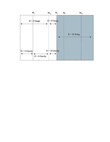
Figure 1: General pattern of mass scales in scenario (1), where the lowest scale is the compactification mass $M_{1}$ and $M_{\omega_{1}}=M_{Planck}$.

Notice that these values of $R_{1}$ and $M_{s}$ drive winding modes with mass $M_{\omega_{c}}$ to be lighter than the string scale, depending on the precise value of $\alpha_{3}$. This, in principle, could have a great phenomenological impact and we will discuss it in full detail in sect. 3.

We recall, however, that such a low value for the string scale could give problems related to the gauge coupling unification [15]. In our scenario, an infinite tower of winding modes of the SM particles arise above $M_{\omega_{c}}$, changing the logarithmic running of the couplings to a power-law running [16]. However, in [17] it was shown that the modified running is not compatible with the available results for $\alpha_{s}(M_{Z})$ imposing unification at the TeV scale.

As a final comment to the low-energy string scale scenario, we consider the problem of SUSY-breaking. If the spontaneous supersymmetry breaking occurs on a distant D$p$-brane other than the one where the SM particles are living in, its effect could be communicated to the visible sector by gravity. The gravitino mass is, then, given by:

$$m_{3/2}\simeq\frac{F}{M_{Planck}}\simeq\frac{M_{s}^{2}}{M_{Planck}}\sim 10^{-13}\ {\rm GeV}\ .$$ (15)

where $F$ is the scale of the SUSY-breaking. The phenomenological implications of such an extremely light gravitino have been considered in [18], where also the lower bounds on $m_{3/2}$ are discussed.

The case in which the smallest scale of the model is the winding mass $M_{\omega_{1}}=10^{-13}\ {\rm GeV}$ is clearly ruled out by experiments. Since this extremely light winding mode would interact with SM particles experimental signatures of this scenario should have been already discovered.

2.2 Middle-energy String Scenario: Planck-Weak scale duality

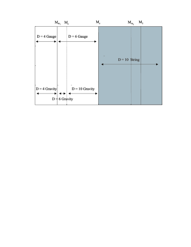
Figure 2: General pattern of mass scales in scenario (1), where the lowest scale is the winding mass $M_{\omega_{1}}$ and $M_{1}=M_{Planck}$.

In this case we fix the string scale, $M_{s}$, in a intermediate region between the weak scale and the Planck scale. We choose, as a reference value, $M_{s}=10^{11}$ Gev. Following our Ansatz, we obtain the two following scenarios whenever $M_{1}$ or $M_{\omega_{1}}$ are taken as large as $M_{Planck}$ and the GUT coupling $\alpha_{3}/\sqrt{2}=10^{-2}$:

$$M_{1}\sim 10^{3}\ {\rm GeV}\quad < \quad M_{\omega_{c}}\sim 10^{10}\ {\rm GeV}\quad<\quad M_{s}\sim 10^{11}\ {\rm GeV}\quad$$ (16)

$$< M_{c}\sim 10^{12}\ {\rm GeV}\quad<\quad M_{\omega_{1}}\sim M_{Planck}=10^{19}$$

and

$$M_{\omega_{1}}\sim 10^{3}\ {\rm GeV}\quad < \quad M_{c}\sim 10^{4}\ {\rm GeV}\quad<\quad M_{s}\sim 10^{11}\ {\rm GeV}\quad$$ (17)

$$< M_{\omega_{c}}\sim 10^{18}\ {\rm GeV}\quad<\quad M_{1}\sim M_{Planck}=10^{19}\ .$$

This two scenarios are graphically shown in Fig. 1 and Fig. 2, respectively. The effect of growing $\alpha_{3}$ is to reduce the splitting within $M_{s}-M_{c}$ and $M_{s}-M_{\omega_{c}}$ in the first case (see Fig. 1) or the splitting $M_{c}-M_{\omega_{1}}$ and $M_{\omega_{c}}-M_{1}$ in the second scenario (see Fig. 2).

The corresponding Isotropic scenario was considered in [5] as a motivation for the large hierarchy between the Planck scale, $M_{Planck}$ and the Weak scale, $M_{Weak}$. In that paper the large hierarchy is just the amplification of the small hierarchy

$$\frac{M_{c}}{M_{s}}\sim\alpha_{3}\sim\alpha_{GUT}=10^{-2}$$ (18)

driven by the $p-6$ exponent of eq. (8). For this scenario to work, the additional constraint is considered:

$$M_{Weak}\sim m_{3/2}\sim\frac{M_{s}^{2}}{M_{Planck}},$$ (19)

where the first relation is motivated by the phenomenological request of having soft masses at the TeV scale. Under our Ansatz, this “Weak-Planck duality” arises naturally choosing the smallest scale at TeV.

Soft terms originating from a TeV-compactification scale have been considered in [19]. In principle, the same mechanism can be applied also for TeV-winding modes. This can be easily understood via a $T_{1}$-duality, thus exchanging $M_{\omega_{1}}$ with $M_{1}$ and replacing the 3-brane with the $5_{1}$-brane.

2.3 High-energy String Scenario

In this case we consider the string scale $M_{s}=M_{GUT}=10^{16}\ {\rm GeV}$. This scenario could be interesting to relate the string scale and the GUT unification scale. Following our Ansatz, we obtain the two following scenarios whenever $M_{1}$ or $M_{\omega_{1}}$ are taken as large as $M_{Planck}$ and the GUT coupling $\alpha_{3}/\sqrt{2}=10^{-2}$:

$$M_{1}\sim 10^{13}\ {\rm GeV}\quad < \quad M_{\omega_{c}}\sim 10^{15}\ {\rm GeV}\quad<\quad M_{s}\sim 10^{16}\ {\rm GeV}\quad$$ (20)

$$< M_{c}\sim 10^{17}\ {\rm GeV}\quad<\quad M_{\omega_{1}}\sim M_{Planck}=10^{19}$$

and

$$M_{\omega_{1}}\sim 10^{13}\ {\rm GeV}\quad < \quad M_{c}\sim 10^{14}\ {\rm GeV}\quad<\quad M_{s}\sim 10^{16}\ {\rm GeV}\quad$$ (21)

$$< M_{\omega_{c}}\sim 10^{18}\ {\rm GeV}\quad<\quad M_{1}\sim M_{Planck}=10^{19}\ .$$

From the phenomenological point of view, the Anisotropic Model does not add any peculiar feature to what already considered in the Isotropic scenario of [12]. Pushing higher the string scale reproduces the well known old heterotic scenario of eq. (11), with a very small splitting between the different compactification/winding scales.

3 Winding Modes and Large Extra Dimensions

In the previous section, we stressed that in the framework of a Type I string theory, many different mass scales arise when Anisotropic Compactification of the 6 extra dimensions is considered. We noticed that quite generally winding modes could appear below the string scale, both when the lowest scale is $M_{1}$ or $M_{\omega_{1}}$. Since winding modes are felt by the gauge interactions is of particular interest to study if they could give observable signatures at the planned accelerators and put bounds on their mass from the existing data. These bounds can be derived in the context of Type I strings without assuming our Ansatz.

We remind that winding modes can be treated just as KK excitations. Although the SM particles are confined in 4D, and thus they do not see the opening of extra dimensions (and therefore they do not possess any KK mode), they still have an infinite tower of massive excitations, corresponding to their winding modes. This means that, for example, the present limits on massive replicas of SM gauge bosons, such as $Z^{\prime}_{SM}$ or $W^{\prime}_{SM}$, can be directly translated into limits on the winding mode mass. As we stressed in sect. 1, this situation is not at all peculiar to a model where the SM particles are confined on a 3-brane. If, for example, we consider a model with closed strings living in 10D and open strings tied to a 9-brane, our results for the winding modes can be directly converted in results for KK modes, as shown in Tab. 1. We found it easier to restrict ourselves to the case where the SM is confined on a 3-brane, but we believe useful to stress again that our results are not at all peculiar to this particular choice.

There are two possible interesting situations where winding modes could play a role in the planned high-energy experiments:

• The lowest mass scale is $M_{\omega_{1}}\simeq 1$ TeV. In this case case, direct searches at present and future accelerators can put a lower limit on $M_{\omega_{1}}$, that within our Ansatz translates into a bound on $M_{s}$. The phenomenological implications of this scenario are quite similar to what was found in [20], where the phenomenology of KK modes at the ${\rm TeV}$-scale was studied in the framework of orbifold compactification of heterotic string theory.

• We have a very large compactification radius, $R_{1}$, and a string scale around 1 TeV. This case has been qualitatively studied in sect. 2.1, where we pointed out that winding modes slightly lighter than the string scale are possible with no need of any particularly strong assumption. However, since mass scales patterns of this type have been extensively studied in the recent literature, we believe this scenario deserves a particular attention.

In the following, we will briefly remind the basic formulae present in the literature and apply them with special attention to the role of the winding modes in the Large Extra Dimensions scenario.

3.1 Phenomenology and experimental constraints

New gravitational experiments [21] could in principle observe deviations from the Einstein-Newton 4D gravity due to extra dimensions down to a compactification radius $R\sim 10\ {\mu\rm m}$. Present gravity experiments test the Newton law down to $R_{exp}\geq 1\ {\rm cm}$. In [7] a scenario was proposed where new extra dimensions arise at the mm-scale affecting gravitational interactions, whereas the SM particles are confined to a 4D space-time. It was noticed in [8] that in the framework of Type I strings this is naturally achieved by considering the SM living on a 3-brane.

It is also possible that new high-energy experiments at the ${\rm TeV}$-scale such as NLC or LHC could observe effects due to the emission of a graviton into the extra dimensions [9]. Although the graviton emission in 4D is suppressed by the 4D Newton constant, $G_{N}=1/M_{Planck}^{2}$, the integration over all the KK modes of the graviton trades this suppression factor with a much smaller one,

$$\frac{1}{M_{Planck}^{2}}\to\frac{E^{n}}{M_{(D)}^{2+n}},$$ (22)

where $n$ is the number of extra dimensions accessible to the graviton, $M_{(D)}$ is the Planck mass in D $=4+n$ dimensions and $E$ is the c.m. energy. If the D-dimensional Planck mass is at the ${\rm TeV}$-scale, graviton production becomes accessible at the planned accelerators. The typical signature will be the production of a SM particle and missing energy [9].

The interest of this scenario relies on the fact that the two relevant scales $R\sim 1\ {\rm mm}$ and $M_{(D)}\sim 1\ {\rm TeV}$ are precisely the scales accessible to gravity and high-energy planned experiments, respectively. Slightly changing these scales dramatically change its experimental appeal for the near future. In particular, the number of extra dimensions felt by gravity at the ${\rm TeV}$-scale and the precise values of $M_{(D)}$ and of the compactification radii, $R_{i}$, are fundamental when making quantitative predictions on the decay rate into gravitons or on a specific cross-section. In the literature, it has been shown that the case with $n=2$ (thus, the scenario considered in this paper) gives the favoured signatures at the planned experiments.

By relating the 4D Newton constant $G_{N}$ with the $D=4+n$ one, we get:

$$M^{2}_{Planck}=8\pi R^{n}M^{n+2}_{(D)}$$ (23)

where $R$ is the radius of $n$ extra dimensions. The Newton constant in Type I strings is also related to the SM gauge coupling, the string scale $M_{s}$ and the compactification scales, $M_{i}$, by eq. (4). Combining these two relations, we get

$$M^{2}_{(6)} = \frac{1}{\sqrt{4\pi}\alpha_{3}}M^{2}_{\omega_{c}},\qquad M_{1}<M_{2}=M_{3}=M_{c}$$

$$M^{3}_{(8)} = \frac{1}{\sqrt{4\pi}\alpha_{3}}M^{2}_{s}M_{\omega_{1}},\qquad M_{2}=M_{3}=M_{c}<M_{1}$$

$$M^{4}_{(10)} = \frac{1}{\sqrt{4\pi}\alpha_{3}}M^{4}_{s},$$ (24)

respectively for $n=2,4,6$ Large Extra Dimensions.

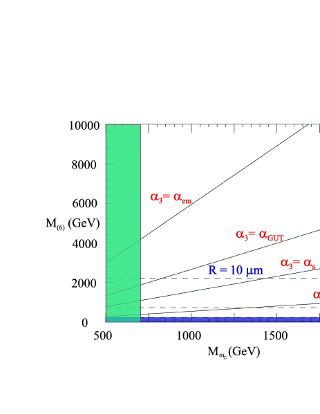
Figure 3: Bounds on $M_{(6)}$ as a function of $M_{\omega_{c}}$ for different values of $\alpha_{3}=\alpha_{em},\alpha_{GUT},\alpha_{s},1$. The dashed lines are the excluded region if no deviation from Newton law is found at $R_{1}=1\ {\rm mm},10\ {\mu\rm m}$. The lower shaded area is the excluded region from present gravitational experiments testing the Newton law down to $R\sim 1\ {\rm cm}$. The vertical left shaded area represent the excluded region from non observation of massive replicas of SM bosons.

This means that in the case $n=2$, for which the most promising experimental signatures are foreseen, the relevant scale in the game is the winding mode mass $M_{\omega_{c}}$. This scale is directly related to the 6-dimensional Planck mass, that is the quantity for which bounds can be extracted by the experiments (see [9]). Notice that in this particular case the string scale is completely irrelevant from the phenomenological point of view and could take any value (above 1 TeV). However, within our Ansatz the string scale could still be related to the winding mode mass:

$$M_{s}^{2}=\frac{\sqrt{2}}{\alpha_{3}}M^{2}_{\omega_{c}}=\sqrt{8\pi}M_{(6)}^{2}$$ (25)

and therefore a lower bound on $M_{\omega_{c}}$ translates into a lower bound for $M_{s}$ also.

By looking to deviations from the Newton law in gravity experiments we can put direct bounds on $R$, that using eq. (23) give limits on $M_{(6)}$. If we use then Type I strings relations, we get from limits on $M_{(6)}$ bounds on the winding mode mass and, within our Ansatz, on $M_{s}$. In Tab. 2 we resume these bounds for typical values of $R$ (with $\alpha_{3}=\alpha_{GUT}$).

$R_{1}$	$M_{(6)}$	$M_{\omega_{c}}$	$M_{s}$
1 ${\rm cm}$	$\geq 220\ {\rm GeV}$	$\geq 80\ {\rm GeV}$	$\geq 490\ {\rm GeV}$
1 ${\rm mm}$	$\geq 700\ {\rm GeV}$	$\geq 270\ {\rm GeV}$	$\geq 1.5\ {\rm TeV}$
10 ${\mu\rm m}$	$\geq 2.2\ {\rm TeV}$	$\geq 840\ {\rm GeV}$	$\geq 5\ {\rm TeV}$

Table 2: Bounds on $M_{(6)},M_{\omega_{c}}$ and $M_{s}$ from present and future gravity experiments, with $\alpha_{3}=\alpha_{GUT}=1/24$. The limit on $M_{(6)}$ is directly derived assuming $4+n$ Newton law. The limit on $M_{\omega_{c}}$ comes from the Type I string relations, whereas the limit on $M_{s}$ is obtained using our Ansatz.

Present experimental limits on $R_{1}\leq 1\ {\rm cm}$ put a very weak lower bound to the winding mode mass.

Existing experimental limits on massive replicas of SM gauge bosons, such as $Z^{\prime}_{SM}$ or $W^{\prime}_{SM}$, can be directly translated into $M_{\omega_{c}}\geq 700$ GeV [22]. This bound can be used to put limits on $R_{1},M_{(6)}$ and $M_{s}$. Using the first formula in eq. (24), with $\alpha_{3}=\alpha_{GUT}=1/24$, we obtain the limit $M_{(6)}\geq 1.8$ TeV. Contextually, using eq. (23), one should also have $R\leq 0.15\ {\rm mm}$.

Non-observation of massive replicas of SM particles at the planned accelerators would imply even stronger bounds on $M_{(6)}$. For example, non-observation at NLC500 (i.e. $M_{Z^{\prime}_{SM}}\geq 5$ Tev) [23], translates into $M_{(6)}\geq 13$ TeV and $R\leq 3\times 10^{-3}\ {\rm mm}$. The dependence of the previous limit on $\alpha_{3}$ is shown in Fig. 3 and Fig. 4.

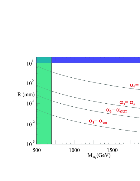
Figure 4: Bounds on $R_{1}$ as a function of $M_{\omega_{c}}$ for different values of $\alpha_{3}=\alpha_{em},\alpha_{GUT},\alpha_{s},1$. The upper shaded area is the excluded region from present gravitational experiments testing the Newton law down to $R\sim 1\ {\rm cm}$. The vertical left shaded area represent the excluded region from non observation of massive replicas of SM bosons.

The Isotropic case $n=6$ provides a direct relationship between $M_{s}$ and the experimentally tested $M_{(10)}$. We face two possibilities:

• We observe deviations from the Newton law at the planned gravitational experiments, $R\sim 1\ {\rm mm}$. In this case, we immediately get $M_{s}\sim 10^{-5}\ {\rm GeV}$ (for $\alpha_{3}=1/24$). Clearly, this situation is excluded by experiments, since the string scale is too low.

• $M_{s}\sim 1\ {\rm TeV}$. In this case we get $M_{c}\sim 10^{-2}\ {\rm GeV}$ (i.e. $R\sim 10^{-11}$ mm), and thus no extra dimensions could be observed at the planned gravity experiments. Moreover, graviton emission phenomena are suppressed with respect to the $n=2$ case, due to the high power of $E^{6}/M^{8}_{(10)}$ to be compared with $E^{2}/M^{4}_{(6)}$. Although this case is not excluded, its lower phenomenological interest with respect to the $n=2$ case is manifest.

Finally, in the $n=4$ case, a limit on $M_{(8)}$ gives a bound on the combination $M^{2}_{s}M_{\omega_{c}}$. This case is, in a certain way, a intermediate situation between the two previous ones.

If the planned experiments do not discover any winding modes, we see that we could put bounds on $M_{(6)}$ and on $R$. However, we could also imagine a situation where new experiments do discover some winding modes. If then we have a new accelerator experiment with c.m. energy above the winding modes threshold, gravity (that feels both KK and winding modes) start to see new extra dimensions of radius $R_{\omega_{c}}=1/M_{\omega_{c}}$. Hence, the Newton constant is again modified:

$$M_{(6)}^{2}=R^{4}_{\omega_{c}}M_{(10)}^{6}$$ (26)

If we now make use of eq. (24), we get:

$$M_{(10)}^{3}=\sqrt{4\pi}\alpha_{3}M_{(6)}^{3}$$ (27)

and thus the suppression factor for graviton emission into the extra dimensions is

$$\frac{1}{M_{(4)}^{2}} \to \frac{E^{2}}{M^{4}_{(6)}}$$

$$\to \frac{E^{6}}{M^{2}_{(6)}M^{6}_{(10)}}\to\frac{E^{6}}{4\pi\alpha_{3}^{2}M^{8}_{(6)}}$$

This means that in this case the suppression factor $E^{6}/M^{8}_{(D)}$ typical of Isotropic compactification of $n=6$ dimensions gets an enhancement factor $1/(4\pi\alpha_{3}^{2})\simeq 50$ (for $\alpha_{3}=1/24$). This enhancement could be relevant when looking for graviton emission into extra dimensions above the winding mode threshold.

If we take into account the present astrophysical and cosmological bounds on $M_{(6)}\geq 30\ {\rm TeV}$, we get: $R_{1}\leq 5\times 10^{-4}\ {\rm mm}$, $M_{\omega_{c}}\geq 12\ {\rm TeV}$ and, within our Ansatz, $M_{s}\geq 70\ {\rm TeV}$.

4 Conclusions

The Anisotropic Compactification scenario of Type I string theory represent the preferred framework for TeV-scale gravity models. However, in this scenario a large number of mass scales naturally appear possibly reintroducing the hierarchy problem and suggesting that a stabilization mechanism of the compactification radii is at work. Moreover, in Type I strings, the string scale is not fixed to a particular value and the Planck mass seems to loose its fundamental role. This situation has to be compared to that of heterotic string theory. In this paper, we considered $M_{Planck}$ to be “dual” to the lowest mass scale of the model. Within this simple assumption, all the mass scales can be deduced by only two free parameters, the gauge coupling $\alpha_{3}$ and one mass scale (for example $M_{s}$). Moreover, the Planck scale recovers a physical meaning. In sect. 2 we analysed qualitatively in the context of our Ansatz the different scenarios that arise for three reference values of $M_{s}=10^{3},10^{11}$ and $10^{16}\ {\rm GeV}$. We noticed that quite generally winding modes could appear below the string scale, thus being of some phenomenological relevance.

In the case of $n=2$ Large Extra Dimension, direct searches of the lightest winding modes can put stringent bounds on both the largest compactification scale, $R_{1}$, and the six-dimensional Planck mass, $M_{(6)}$. We stress that these results are completely independent from our Ansatz and follows only by assuming Type I string theory. With the present data on massive replicas of SM gauge bosons, $M_{Z^{\prime}_{SM}}\geq 700\ {\rm GeV}$, we obtain $M_{(6)}\geq 1.8\ {\rm TeV}$ and $R_{1}\leq 0.15\ {\rm mm}$ for a reasonable value of $\alpha_{3}$. Search for direct production of winding modes at LHC or NLC can then represents a useful tool to explore the parameter space of Large Extra Dimension models derived from Type I string theory and give a possibly cleaner signature than graviton emission into the bulk.

The phenomenology of winding modes is quite interesting and deserves a careful study.

References

- [1] K. Dienes, Phys. Rept. 287 (1997) 447.
- [2] E. Witten, Nucl. Phys. B 471 (1996) 135.
- [3] J. Polchinski and E. Witten, Nucl. Phys. B460 (1996) 525.
- [4] P. Horawa and E. Witten, Nucl.Phys. B460 (1996) 506.
- [5] C. Burgess, L. Ibáñez and F. Quevedo, hep-ph/9810535.
- [6] J. D. Lykken, Phys. Rev. D54 (1996) 3693.
-
[7]
N. Arkani-Hamed, S. Dimopoulos and G. Dvali,
Phys. Lett. B 429 (1998) 263;
N. Arkani-Hamed, S. Dimopoulos and G. Dvali, hep-ph/9807344. -
[8]
I. Antoniadis, N. Arkani-Hamed, S. Dimopoulos and G. Dvali,
Phys. Lett. B 436 (1998) 257;
G. Shiu and S. -H. H. Tye, Phys. Rev. D58 (1998) 106007. -
[9]
G. Giudice, R. Rattazzi and J. Wells, hep-ph/9811291;
E.A. Mirabelli, M. Perelstein and M. E. Peskin, hep-ph/9811337;
T. Han, J. D. Lykken and R.J. Zhang, hep-ph/9811350. - [10] For a review see J. Polchinski, hep-th/9611050 and C.P. Bachas hep-th/9806199.
-
[11]
For reviews and references see :
F. Quevedo, Nucl. Phys. (Proc. Suppl. ) 62 (1998) 134;
F. Quevedo, hep-th/9603074;
J. Lykken, Nucl. Phys. (Proc. Suppl. ) 52 A (1997) 271;
Z. Kakushadze and S.-H. H. Tye, hep-th/9512155;
G. Aldazabal, hep-th/9507162;
L. Ibáñez, hep-th/9505098. - [12] L. Ibáñez, C. Muñoz and S. Rigolin, hep-th/9812397.
-
[13]
N. Arkani-Hamed, S. Dimopoulos and J. March-Russell, hep-th/9809124;
K.R. Dienes, E. Dudas, A. Gherghetta and A. Riotto, hep-ph/9809406;
D. Lyth, hep-ph/9810320;
N. Kaloper and A. Linde, hep-th/9811141;
G. Dvali and S. -H. H. Tye, hep-ph/9812483. -
[14]
Z. Kakushadze and S. -H. H. Tye, hep-th/9809147;
K. Benakli, hep-ph/9809582;
M. Maggiore and A. Riotto, hep-th/9811089;
S. Nussinov and R. Shrock, hep-ph/9811323;
N. Arkani-Hamed and S. Dimopoulos, hep-ph/9811353;
J. Hewett, hep-ph/9811356;
Z. Berezhiani and G. Dvali, hep-ph/9811378;
K.R. Dienes, E. Dudas and A. Gherghetta, hep-ph/9811428;
N. Arkani-Hamed, S. Dimopoulos and J. March-Russell, hep-ph/9811448;
P. Mathews, S. Raychaudhuri and K. Sridhar, hep-ph/9811501; hep-ph/9812486;
Z. Kakushadze, hep-th/9812163;
A. E. Faraggi and M. Pospelov, hep-ph/9901299. - [15] E. Caceres, V. S. Kaplunovsky and I. M. Mandelberg, Nucl. Phys. B 493 (1997) 73.
-
[16]
T.R. Taylor and G. Veneziano, Phys. Lett. B 212 (1988) 147;
K.R. Dienes, E. Dudas and A. Gherghetta, Phys. Lett. B 436 (1998) 55; Nucl. Phys. B 537 (1999) 47;
S. Abel and S. King, hep-ph/9809467. -
[17]
G. Ghilencea and G.G Ross, Phys. Lett. B 442 (1998) 165;
T. Kobayashi, J. Kubo, M. Mondragon and G. Zoupanos, hep-ph/9812221. -
[18]
A. Brignole, F. Feruglio and F. Zwirner, Nucl. Phys. B 516 (1998) 13;
A. Brignole, F. Feruglio, M. L. Mangano and F. Zwirner, Nucl. Phys. B 526 (1998) 136;
A. Brignole, F. Feruglio and F. Zwirner, Phys. Lett. B 438 (1998) 89. -
[19]
I. Antoniadis, S. Dimopoulos, A. Pomarol and M. Quiros, hep-ph/9810410;
A. Delgado, A. Pomarol and M. Quiros, hep-ph/9812489. -
[20]
I. Antoniadis, Phys. Lett. B 246 (1990) 377;
I. Antoniadis, C. Muñoz and M. Quirós, Nucl. Phys. B 397 (1993) 515;
I. Antoniadis, K. Benakli and M. Quirós, Phys. Lett. B 331 (1994) 313. -
[21]
J. C. Price, in Proc. Int. Symp. on Experimental Gravitational Physics,
ed. P. F. Michelson, Guangzhou, China (World Scientific, Singapore, 1988);
J. C. Price et al., NSF proposal, 1996;
A. Kapitulnik and T. Kenny, NSF proposal, 1997;
J. C. Long, H. W. Chan and J. C. Price, Nucl. Phys. B 539 (1999) 23. -
[22]
S. Abachi et al., D0 Collaboration,
Phys. Rev. Lett. 76 (1996) 3271;
F. Abe et al., CDF Collaboration, Phys. Rev. Lett. 79 (1997) 2192. - [23] See, for example, A. Leike and S. Riemann, Z. Phys. C75 (1997) 341.