1 Introduction

The calculation of diagrams with one non-zero external momentum squared ($q^{2}$) has wide applications in QED and QCD for both selfenergies and vertices. In these cases also only one non-zero mass enters the problem. In electroweak problems like $Z\to b\bar{b}$ one has mixing terms between electroweak and strong interactions and due to that different internal masses occur, so that the method of Taylor expansion is getting more difficult to apply. In this case, however, the top quark ($m_{t}$) plays a special role and it allows to make the expansion in the large mass. The method is not applicable to arbitrary high $q^{2}$, but as has been demonstrated in $\!{}^{{\bf?}}$, for $q^{2}=m_{Z}^{2}$ this approach is still reliable. While in $\!{}^{{\bf?}}$ only scalar diagrams have been considerd, here we investigate the full decay amplitude. It turns out that the obtained results are simpler for the full process than for scalar diagrams in the following sense: first of all, complicated functions like higher polylogarithms, which show up in the analytic evaluation of scalar diagrams, cancel in the full amplitude; furthermore the convergence of the large mass expansion also turns out to be better for the full amplitude than for scalar diagrams. These observations are manifestation of gauge cancellations observed in gauge theories in general. Nevertheless their observation in this special form is surprising!

Due to the fact that the method of mapping and Taylor expansion is quite useful and finds applications by other authors (see e.g. $\!{}^{{\bf?}}$), we give a short review here concerning the method and report on recent developements of calculating Taylor coefficients for two-loop diagrams. Then, in the second part, we turn to our main point namely the large mass expansion for the $Z\to b\bar{b}$ problem and the comparison with the work of $\!{}^{{\bf?}}$.

2 Expansion of three-point functions in terms of an external momentum squared

Taylor series expansions in terms of one external momentum squared, $q^{2}$ say, were considered for selfenergy diagrams in $\!{}^{{\bf?}}$, Padé approximants were introduced in $\!{}^{{\bf?}}$ and in Ref. $\!{}^{{\bf?}}$ it was demonstrated that this approach can be used to calculate Feynman diagrams on their cut by analytic continuation. In the case of a three-point function like $Z\to b\bar{b}$ in the $m_{b}=0$ limit we have for the external $b-$quark momenta $p^{2}_{1}=p^{2}_{2}=0$. The expansion of the scalar diagram then looks like

$$C(p_{1},p_{2})=\sum^{\infty}_{n=0}a_{n}(p_{1}p_{2})^{n},$$ (1)

with $q^{2}=(p_{1}+p_{2})^{2}.$

For the calculation of the Taylor coefficients in general various procedures have been proposed $\!{}^{{\bf?},{\bf?},{\bf?}}$. These methods are well suited for programming in terms of a formulae manipulating language like FORM $\!{}^{{\bf?}}$. Such programs, however, yield acceptable analytic results only in cases when not too many parameters (like masses) enter the problem. Otherwise numerical methods are needed $\!{}^{{\bf?}}$.

In the case of only one non-zero mass and only one external momentum squared, indeed the case with the least nontrivial parameters, for many diagrams analytic expressions for the Taylor coefficients can be obtained. For recent references see $\!{}^{{\bf?}}$.

For the purpose of calculating Feynman diagrams in the kinematical domain of interest it is necessary to calculate them from the Taylor series on their cut. This is performed by analytic continuation in terms of a mapping $\!{}^{{\bf?}}$

Assume, the following Taylor expansion of a scalar diagram or a particular amplitude is given $C(p_{1},p_{2},\dots)=\sum^{\infty}_{m=0}a_{m}y^{m}\equiv f(y)$ and the function on the r.h.s. has a cut for $y\geq y_{0}$.

The method of evaluation of the original series consists in a first step in a conformal mapping of the cut plane into the unit circle and secondly the reexpansion of the function under consideration into a power series w.r.t. the new conformal variable. We use

$$\omega=\frac{1-\sqrt{1-y/y_{0}}}{1+\sqrt{1-y/y_{0}}}.$$ (2)

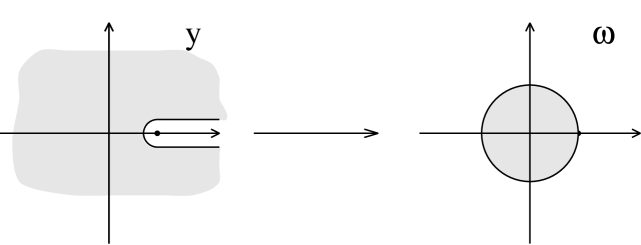
Figure 1: Conformal mapping of the complex y-plane into the $\omega$-plane.

By this conformal transformation, the $y$-plane, cut from $y_{0}$ to $+\infty$, is mapped into the unit circle (see Fig.1) and the cut itself is mapped on its boundary, the upper semicircle corresponding to the upper side of the cut. The origin goes into the point $\omega=0$.

After conformal transformation it is suggestive to improve the convergence of the new series w.r.t. $\omega$ by applying the Padé method $\!{}^{{\bf?},{\bf?}}$. A convenient technique for the evaluation of Padé approximations is the $\varepsilon$-algorithm of $\!{}^{{\bf?}}$ which allows one to evaluate the Padé approximants recursively.

Generally speaking, the precision of results with this mapping and Padé is of the order of 3-4 decimals with 30 Taylor coefficients for timelike $q^{2}$ values a factor of approximately 100 times the lowest threshold value. For lower $q^{2}$ (a few times the threshold value) the precision is of the order of 10 decimals in quite many cases. The precision worsens near second nonzero thresholds.

As a final remark we mention that for diagrams with zero thresholds new techniques have been developed. In fact terms of the form $\ln^{m}(q^{2})$ have to be factorized, where $m$ is the number of zero thresholds of the diagram. The factors in front are then expanded in terms of Taylor series $\!{}^{{\bf?},{\bf?}}$.

3 Large Mass Expansion (LME)

As mentioned above, for the evaluation of diagrams with several different masses, one of which being large (like the top mass $m_{t}$), we use the general method of asymptotic expansion in large masses $\!{}^{{\bf?}}$. For a given scalar graph $G$ the expansion in large mass is given by the formula

$$F_{G}(q,M,m,\varepsilon)\stackrel{{\scriptstyle M\to\infty}}{{\sim}}\sum_{\gamma}F_{G/\gamma}(q,m,\varepsilon)\circ T_{q^{\gamma},m^{\gamma}}F_{\gamma}(q^{\gamma},M,m^{\gamma},\varepsilon),$$ (3)

where $\gamma$’s are subgraphs involved in the asymptotic expansion, $G/\gamma$ denotes shrinking of $\gamma$ to a point; $F_{\gamma}$ is the Feynman integral corresponding to $\gamma$; $T_{q_{\gamma},m_{\gamma}}$ is the Taylor operator expanding the integrand in small masses $\{m_{\gamma}\}$ and external momenta $\{q_{\gamma}\}$ of the subgraph $\gamma$ ; $\circ$ stands for the convolution of the subgraph expansion with the integrand $F_{G/{\gamma}}$. The sum goes over all subgraphs $\gamma$ which (a) contain all lines with large masses, and (b) are one-particle irreducible w.r.t. light lines.

For the $Z\to b\bar{b}$ decay we have $q^{2}=M_{Z}^{2}$ for the on-shell $Z$’s. Fig.2 shows diagrams with two different masses on virtual lines, one of which a top. $W$ and $Z$ are the gauge bosons with masses $M_{W}$ and $M_{Z}$, respectively; $\phi$ is the charged would-be Goldstone boson (we use the Feynman gauge); $t$ and $b$ are the t- and b-quarks. Fig. 3 shows subdiagrams needed in the expansion (3).

Figure 2: Two-loop diagrams with two different masses on internal lines arising in $Zb\overline{b}$.

Figure 3: The structure of the LME, see explanations in the text.

Finally the LME of the above diagrams has the following general form

$$F_{\rm as}^{N}=\frac{1}{m_{t}^{4}}\sum_{n=-1}^{N}\sum_{i,j=-1;i+j=n}^{n}\left(\frac{M_{W}^{2}}{m_{t}^{2}}\right)^{i}\left(\frac{q^{2}}{m_{t}^{2}}\right)^{j}\sum_{k=0}^{m}A_{i,j,k}(q^{2},M_{W}^{2},{\mu}^{2})\ln^{k}\frac{m_{t}^{2}}{\mu^{2}}$$ (4)

where $m$ is the highest degree of divergence (ultraviolet, infrared, collinear) in the various contributions to the LME ($m\leq$ 3 in the cases considered). $M_{W}^{2}/m_{t}^{2}$ and $q^{2}/m_{t}^{2}$ are considered as small parameters. $A_{i,j,k}$ are in general complicated functions of the arguments, i.e. they may contain logarithms and higher polylogarithms.

In contrary to the work of $\!{}^{{\bf?}}$ we see no inconveniences in directly applying the above method and did not use any “continued expansion”.

In the following we present some of our results of the LME for the full two-loop $O(\alpha\alpha_{s})$ contribution. As in $\!{}^{{\bf?}}$, we are interested only in the virtual effect of the top quark, which renders the decay of the $Z$ boson into bottom quarks different from the one into other down-type quarks. Therefore in the following the quantity $\Gamma_{b-d}^{W}=\Gamma_{Z\to bb}^{W}-\Gamma_{Z\to dd}^{W}$ is considered in two loop order, in which expression the counterterm contributions cancel. The superscript $W$ means that only diagrams with virtual $W$ bosons are included. The other part with the $Z$ exchange makes no discrimination between $b$- and $d$-quarks and is calculated in order $\alpha\alpha_{s}$ in $\!{}^{{\bf?}}$. Our result reads

$$\delta\Gamma_{b-d}^{(2),W}=\Gamma^{0}{1\over s_{\Theta}^{2}}{\alpha\over\pi}\frac{\alpha_{s}}{\pi}\times$$ (5)

$$\mbox{}\bigg{\{}{M_{t}^{2}\over M_{W}^{2}}\,\bigg{[}-{1\over 32}-{1\over 64}\,{1\over y}+\zeta_{2}\,\bigg{(}{1\over 16}+{1\over 32}\,{1\over y}\bigg{)}\bigg{]}$$

$$\mbox{}+\bigg{[}\frac{61}{288}\frac{1}{y}+\frac{82661}{466560}-\frac{106626671}{204120000}y+\frac{673933}{1458000}y^{2}-\frac{12334491149}{16044682500}y^{3}+{\cal O}(y^{4})$$

$$\mbox{}\hskip 10.00002pt+I_{1}\,\biggl{(}\frac{1}{96}\frac{1}{y^{2}}-\frac{5}{192}\frac{1}{y}-\frac{5}{48}-\frac{1}{48}y\biggr{)}$$

$$\mbox{}\hskip 10.00002pt+\zeta_{2}\,\bigg{(}{173\over 1296}+{67\over 2592}\,{1\over y}+{53\over 324}\,y\bigg{)}+\zeta_{3}\,\bigg{(}-{1\over 18}\,{1\over y}+{7\over 90}\,y-{1\over 45}\,y^{2}-{16\over 315}\,y^{3}\bigg{)}$$

$$\mbox{}\hskip 10.00002pt+L_{tW}\,\bigg{(}-{757\over 7776}-{331\over 7776}\,{1\over y}-{95\over 3888}\,y\bigg{)}+l_{\Theta}^{2}\,\bigg{(}-{103\over 2592}-{1\over 81}\,{1\over y}+{1\over 300}\,y$$

$$\mbox{}\hskip 10.00002pt-{103\over 1080}\,y^{2}-{5314\over 33075}\,y^{3}\bigg{)}+l_{\Theta}\,\bigg{(}-{527\over 7776}+{11\over 288}\,{1\over y}-{1489\over 30375}\,y+{1081\over 9720}\,y^{2}$$

$$\mbox{}\hskip 10.00002pt-{3338578\over 10418625}\,y^{3}\bigg{)}\bigg{]}$$

$$\mbox{}+{M_{W}^{2}\over M_{t}^{2}}\,\bigg{[}\frac{5}{128}\frac{1}{y}-\frac{64847}{1555200}-\frac{636239}{777600}y-\frac{12497}{10800}y^{2}$$

$$\mbox{}\hskip 10.00002pt+I_{1}\,\biggl{(}-\frac{11}{288}\frac{1}{y^{2}}-\frac{253}{864}\frac{1}{y}-\frac{11}{48}+\frac{11}{24}y+\frac{11}{108}y^{2}\biggr{)}$$

$$\mbox{}\hskip 10.00002pt+L_{tW}\,\bigg{(}-{83083\over 155520}-{1819\over 5184}\,{1\over y}+{15017\over 38880}\,y+{3977\over 38880}\,y^{2}\bigg{)}+l_{\Theta}\,\bigg{(}-{3343\over 155520}-{7\over 1296}\,{1\over y}$$

$$\mbox{}\hskip 10.00002pt-{823\over 38880}\,y+{17\over 38880}\,y^{2}\bigg{)}+\zeta_{2}\,\bigg{(}{257\over 864}+{175\over 864}\,{1\over y}+{13\over 144}\,y+{11\over 18}\,y^{2}\bigg{)}\bigg{]},$$

where $\Gamma^{0}$ is the Born decay rate, $y=M_{Z}^{2}/4M_{W}^{2}$, $l_{\Theta}=\ln\cos\Theta_{W}$, $L_{tW}=\ln(m_{t}^{2}/M_{W}^{2})$ and $\zeta_{n}=\zeta(n)$ the Riemann $\zeta$-function. The following integral is introduced

$$I_{n}=\frac{1}{2}\frac{(-1)^{n}}{n!}\int\limits_{0}^{1}\frac{{\ln^{n}(1-ty)}}{\sqrt{1-t}}\,dt\,.$$ (6)

In the above final result enters only $I_{1}$ which has the expansion

$$I_{1}=\frac{2}{3}y+\frac{4}{15}y^{2}+\frac{16}{105}y^{3}+\frac{32}{315}y^{4}+\frac{256}{3465}y^{5}+\frac{512}{9009}y^{6}+\frac{2048}{45045}y^{7}+\frac{4096}{109395}y^{8}+\dots$$ (7)

Inserting this expansion in (5), we fully agree with the result of Harlander et.al. $\!{}^{{\bf?}}$, as far as they have presented their result. Our result is more compact, however, and it is interesting to observe that, while higher polylogarithms occur in the scalar integrals $\!{}^{{\bf?}}$, in the full decay amplitude these and the higher $I_{n}$ (also, however, expressible in terms of polylogarithms) cancel. The remaining $I_{1}$, expanded above, is merely a logarithm: $I_{1}=2-a\log\bigl{(}(a+1)/(a-1)\bigr{)},a=\sqrt{1-1/y}$. Thus we observe that the final result is much simpler than intermediate results from scalar diagrams. Moreover, the convergence of the series in terms of large masses is much better than for the series obtained for scalar diagrams $\!{}^{{\bf?}}$, which is demonstrated below.

Our numerical results are as follows: $x_{1}$ and $x_{2}$ being the 1-loop and 2-loop results, $r=M_{W}^{2}/m_{t}^{2}$, the large mass expansion is given in the form

$$\delta\Gamma_{b-d}^{W} = \Gamma^{0}\frac{1}{s_{\Theta}^{2}}\frac{\alpha}{\pi}\Biggl{[}x_{1}+\frac{\alpha_{s}}{\pi}x_{2}\Biggr{]},$$ (8)

$$x_{1} = \Biggl{(}-\frac{0.1063}{r}\Biggr{)}+\Biggl{(}0.2360-1.0236r-1.7492r^{2}-1.4477r^{3}-0.1758r^{4}+1.2997r^{5}$$ (9)

$$+ 2.1005r^{6}+1.7986r^{7}+0.5692r^{8}-0.9260r^{9}-1.6273r^{10}\Biggr{)}\,,$$

$$x_{2} = \Biggl{(}\frac{0.2435}{r}\Biggr{)}+\Biggl{(}0.7167-1.6940r-4.0920r^{2}-4.7543r^{3}-2.9143r^{4}+0.5688r^{5}$$ (10)

$$+ 3.7747r^{6}+4.8688r^{7}+3.6932r^{8}+4.5196r^{9}+24.090r^{10}\Biggr{)}\,.$$

The first terms in $x_{1},x_{2}$ correspond to the leading $m_{t}^{2}/M_{W}^{2}$. For $m_{t}=175$GeV, $M_{W}=80.33$GeV and $M_{Z}=91.187$GeV we obtain

$$\delta\Gamma^{W}_{b-d}=\Gamma^{0}\frac{1}{s_{\Theta}^{2}}\frac{\alpha}{\pi}\Biggl{[}-0.5045-0.0704+\frac{\alpha_{s}}{\pi}\bigl{(}1.1556+0.1285\bigr{)}\Bigg{]}$$ (11)

In each of these terms the leading term and the corrections are given separately. Note that the leading $m_{t}^{2}/M_{W}^{2}$ term in order $O(\alpha\alpha_{s})$ was obtained earlier in $\!{}^{{\bf?}}$.

The observation is that the series for the full amplitude converges like  $r^{n}$ while for the scalar diagram the convergence was like  $(4r)^{n}$. Accordingly the term of order $r^{4}$ gives only an error of order 0.5% while for the scalar diagrams the errors where of the order several % $\!{}^{{\bf?}}$.

References

- [1] J.Fleischer, M. Kalmykov and O. Veretin, Phys.Lett. B427 (1998) 141.
- [2] See e.g. H. Kühn, these proceedings.
- [3] R.Harlander, T.Seidensticker and M.Steinhauser, Phys. Lett. B426, 125 (1998) ; see also R. Harlander in Zeuthen workshop on Elementary Particle Theory, Acta Physica Polon. 29 (1998) 2691.
- [4] D.J. Broadhurst, Z.Phys., C47 (1990) 115; A.I. Davydychev and J.B. Tausk, Nucl. Phys. B397 (1993) 123; F.A. Berends, A.I. Davydychev and V.A. Smirnov, Nucl. Phys. B478 (1996) 59.
- [5] D.J. Broadhurst, J. Fleischer and O.V. Tarasov, Z.Phys. C60 (1993) 287.
- [6] J. Fleischer and O.V. Tarasov, Z.Phys. C64 (1994) 413.
- [7] J.Fleischer and O.V.Tarasov, in proceedings of the ZiF conference on Computer Algebra in Science and Engineering, World Scientific 1995, ed. J. Fleischer, J. Grabmeier, F.W.Hehl and W.Küchlin.
- [8] A.I. Davydychev and J.B. Tausk, Nucl. Phys. B465 (1996) 507.
- [9] O.V. Tarasov, Nucl. Phys. B480 (1996) 397; Phys.Rev. D54 (1996) 6479.
- [10] J.A.M. Vermaseren: Symbolic manipulation with FORM, Amsterdam, Computer Algebra Nederland, 1991.
- [11] J. Fleischer, Int.J.Mod.Phys. C6 (1995) 495; J.Fleischer et al., Eur.Phys.J. C2 (1998) 747.
- [12] J. Fleischer, A.V. Kotikov and O.L. Veretin, Phys.Lett. B417 (1998) 163; J. Fleischer, A.V. Kotikov and O.L. Veretin, hep-ph/9808242 (to be published in Nucl. Phys.).
- [13] G.A. Baker, Jr., Essentials of Padé Approximants, pp Academic Press (1975).
- [14] D. Shanks, J. Math. Phys. 34 (1955); P. Wynn, Math. Comp. 15 (1961) 151; G.A. Baker, P. Graves-Morris, Padé approximants, in Encyl.of math.and its appl., Vol. 13, 14, pp Addison-Wesley (1981).
- [15] F.A. Berends et al., Nucl. Phys. B439 (1995) 536; J. Fleischer, V. A. Smirnov and O. V. Tarasov, Z.Phys.C74 (1997) 379.
- [16] F.V. Tkachov, Preprint INR P-0332, Moscow (1983); P-0358, Moscow 1984; K.G. Chetyrkin, Teor. Math. Phys. 75 (1988) 26; ibid 76 (1988) 207; Preprint, MPI-PAE/PTh-13/91, Munich (1991); V.A. Smirnov, Comm. Math. Phys.134 (1990) 109;
- [17] A.L. Kataev, Phys.Lett. B287 (1992) 209; A. Czarnecki and J.H. Kühn, Phys.Rev.Lett. 77 (1996) 3955; A. Czarnecki and K. Melnikov, Phys. Rev. D56 (1997) 1638.
- [18] J. Fleischer, O.V. Tarasov, F. Jegerlehner and P. Ra̧czka, Phys. Lett. B293 (1992) 437; G. Buchalla and A.J. Buras, Nucl. Phys. B398 (1993) 285; G. Degrassi, Nucl. Phys. B407 (1993) 271; K.G. Chetyrkin, A. Kwiatkowski and M. Steinhauser, Mod. Phys. Lett. A8 (1993) 2785.